Article

Space Debris Removal: A Game Theoretic Analysis

1
Department of Computer Science, University of Liverpool, Liverpool L69 3BX, UK
2
DFKI GmbH, 28359 Bremen, Germany
3
Advanced Concepts Team, European Space Agency, 2201 AZ Noordwijk, The Netherlands
*
Authors to whom correspondence should be addressed.
Games 2016, 7(3), 20; https://doi.org/10.3390/g7030020
Submission received: 6 June 2016 / Revised: 22 July 2016 / Accepted: 2 August 2016 / Published: 11 August 2016
(This article belongs to the Special Issue Real World Applications of Game Theory)

Abstract

:
We analyse active space debris removal efforts from a strategic, game-theoretical perspective. Space debris is non-manoeuvrable, human-made objects orbiting Earth, which pose a significant threat to operational spacecraft. Active debris removal missions have been considered and investigated by different space agencies with the goal to protect valuable assets present in strategic orbital environments. An active debris removal mission is costly, but has a positive effect for all satellites in the same orbital band. This leads to a dilemma: each agency is faced with the choice between the individually costly action of debris removal, which has a positive impact on all players; or wait and hope that others jump in and do the ‘dirty’ work. The risk of the latter action is that, if everyone waits, the joint outcome will be catastrophic, leading to what in game theory is referred to as the ‘tragedy of the commons’. We introduce and thoroughly analyse this dilemma using empirical game theory and a space debris simulator. We consider two- and three-player settings, investigate the strategic properties and equilibria of the game and find that the cost/benefit ratio of debris removal strongly affects the game dynamics.

Graphical Abstract

1. Introduction

In this work, we apply empirical game theoretic methods to study the strategic real-world problem of space debris removal. The complexity of the space debris environment typically prohibits direct game theoretic analysis. However, by defining appropriate heuristic strategies and using a suitable simulator, we can estimate heuristic payoff functions to model the strategic dilemma as a game. This then enables us to apply (evolutionary) game theoretic analysis.
Since the late 1950s, space agencies have launched many objects into Earth orbits with low or no incentive to remove them after their life span. Due to this, there are now many inactive objects orbiting Earth, which can pose a risk to active spacecraft. By far, the highest spatial density of such objects is in the Low Earth Orbit (LEO) environment, defined as the region of space around Earth with an altitude of 160 km–2000 km. The density of objects in LEO will most likely increase due to new launches, on-orbit explosions and object collisions.
NORAD tracks and catalogues objects in orbit, currently listing around 15,000 objects of 10 cm 2 and larger [1]. However, it is estimated that the true number of objects is several orders of magnitude larger, with estimates of over 100,000 pieces of untracked debris of sizes of 1–10 cm 2 [2]. At orbital speeds of approximately 7.5 km/s, such small pieces can cause considerable damage to active satellites.
In recent years, there have been several incidents producing a high number of debris. Two of them have been especially severe: (i) a 2007 Chinese anti-satellite missile test producing more than 1200 catalogued pieces of debris and an estimated 35,000 pieces of a size of 1 cm and larger, resulting in the most severe orbital debris cloud in history [3]; (ii) the collision of the Iridium-33 and Kosmos-2251 satellites in 2009, which was the first accidental hyper-velocity collision of two intact spacecraft [4]. More than 823 debris objects were catalogued, forming two debris clouds in LEO. This incident introduced a high risk of potential collisions to many active objects in LEO. For example, the International Space Station (ISS) had to perform a manoeuvre in March 2011 to avoid a piece of debris from the 2009 Iridium-Kosmos collision [5].
These two incidents show that space debris is a serious problem with potentially disastrous consequences. As a result, space agencies are now investigating ways in which end-of-life satellites can be safely de-orbited. However, measures that apply only to newly-launched spacecraft may not be sufficient to prevent an exponential build-up of debris. Therefore, active space debris removal becomes relevant. An active debris removal mission has a positive effect (or risk reduction) for all satellites in the same orbital band. This leads to a dilemma: each agency has an incentive to delay its actions and wait for others to respond.
We model this scenario as a non-cooperative game between self-interested agents in which the agents are space agencies. Using a high-fidelity simulator, we estimate payoffs to agents for different combinations of actions taken and analyse the resulting game in terms of best-response dynamics and (Nash) equilibria. Contrary to the urgency of the space debris dilemma, there has not been much attention to this problem in scientific circles. To the best of our knowledge, we are the first to consider this dilemma in the context of multi-agent strategic decision making using empirical game theoretic techniques.
This paper proceeds as follows. We firstly position our study in the context of related work. Next, we present our space debris simulator, which includes a collision model, a break-up model and an orbital propagator. We then outline our game theoretic methodology. Using our simulator, we analyse the potential impact of several removal strategies on the orbital environment and present a game theoretic analysis.

2. Related Work

Our study can be placed in the context of two different areas of related work. Firstly, from a simulation modelling perspective, various attempts have been made to accurately predict the evolution of space debris and the resulting risk of collisions for active space craft. Secondly, from a game theoretic perspective, researchers have utilized similar methods to study related problems of environmental pollution and the shared exploitation of scarce resources [6].
One of the earliest analyses of the projected evolution of space debris was done by Donald J. Kessler in 1978 [7,8]. This study led to the definition of the “Kessler syndrome”, a particular scenario where the density of objects in LEO becomes high enough to cause a cascade of collisions, each producing new debris and eventually saturating the environment, rendering future space missions virtually impossible. Follow-up studies have been published mostly by scientists from NASA, the most well known being the work of Jer C. Liou and Nicholas L. Johnson [9,10,11], in which the authors consider active removal strategies to mitigate the space debris problem.
Liou and Johnson [9] present a sensitivity analysis of object removal strategies. They propose removing 5, 10 or 20 objects per year, which can be seen as a single-agent approach. The authors compare these mitigation strategies with baselines “business as usual” or “no new launches” and show the effectiveness of object removals. The objects to be removed are chosen according to their mass and collision probability. We base our study on Liou and Johnson’s approach, but in contrast consider a multi-agent scenario in which different space agencies independently choose their removal strategy. In our model, we implement individualised object removal criteria based on potential risk to important assets of each of the agents.
The space debris removal dilemma is in many ways similar to other environmental clean-up efforts that have been studied using game theoretic tools in the past. For example, Tahvonen models carbon dioxide abatement as a differential game, taking into account both abatement costs and environmental damage [6]. More complex models have been studied, as well, including for example the ability to negotiate emission contracts [12]. Another related model is the Great Fish War of Levhari and Mirman [13]. Although not the same as environmental clean-up, this scenario deals with shared use of a scarce common resource, which potentially leads to the same dilemma in game theoretic terms, known as the “tragedy of the commons” [14]. However, each of these studies has focused solely on a (simplified) mathematical model of the underlying system. In contrast, we use a complex simulator to obtain an approximate model using empirical game theoretic methods.
Analysis of complex strategic interactions using game theoretic tools is often hindered by the large action-spaces available to the agents in such scenarios. For example, in the space debris removal dilemma, each possible piece of debris to remove is potentially an action. Additionally, it is often impossible to define payoffs to all (combinations of) actions in advance. This has led recently to the advent of empirical game theory [15,16]. The main idea is to limit the strategy space of each agent by introducing high level generic profiles, or meta-strategies, that capture the main aspects of the interaction. Then, the payoff table for this reduced strategy space can be estimated empirically, either by analysing data from a real system or by simulating a model of the system. Standard methods and techniques from (evolutionary) game theory can then be applied to the estimated payoff table, e.g., to find approximate equilibria [17].
Such empirical game theoretic analysis has proven valuable in getting insights into various complex real-world domains, such as automated trading [18], auction mechanism design [19], the game of poker [20], collision avoidance in multi-robot systems [21], adaptive cyber-defence strategies [22] and large-scale bargaining [23]. In this work, we follow a similar approach, but focus on the domain of space debris removal.

3. Space Debris Simulation Model

Our simulator is built on top of the Python scientific library PyKep [24], which provides basic tools for astrodynamics research, such as satellite orbit propagators. To simulate the future development of space debris in Low Earth Orbit (LEO), we develop several sub-modules, including a collision model and a break-up model, which we describe below.
The input data to our model come from two satellite catalogues/databases: (i) the SATCAT 1 database containing descriptions of all objects on Earth orbits that have ever been documented; and (ii) the TLE (Two-Line Element set) 2 database providing up-to-date information on all active (not decayed) objects on Earth orbits, including the orbital elements, which uniquely identify an object’s orbit and which are used for orbit propagation.

3.1. Collision Model

To evaluate the probability of collision between objects, we follow the Cube approach [25]. The Cube approach samples uniformly in time rather than space and is thus compatible with any orbital evolution simulation, as it does not impose assumptions on the orbital geometry. This is particularly important in LEO, where orbital progression is significant in the considered time frame. We use the SGP4 [26] orbital propagator to calculate the evolution of the ephemeris (i.e., position and velocity) of an orbiting object given its TLE description. The ephemerides of all objects are calculated at regular time intervals. Space is then partitioned by a regular 3D-lattice, and for any pair i , j of objects that fall into the same volume, the collision probability is evaluated as follows:
p i , j = s i s j V r e l σ U
where s i = s j are the spatial densities of object i and j in the cube, σ = π ( r i + r j ) 2 is the cross-sectional collision area, V r e l is the collision (relative) velocity of the two objects and U is the volume of the cube. For each pair, a pseudo-random number x is generated from a uniform distribution over the interval [ 0 , 1 ) ; if p i , j > x , a collision event is triggered.

3.2. Breakup Model

We use NASA’s standard breakup model [27] to generate the population of fragments resulting from a collision event. The NASA/JSC breakup model represents a widely-accepted understanding of the fragmentation process of in-orbit collisions and explosions based on multiple ground tests and radar observations of past events.
The model provides distributions for the size, mass and ejection velocity of the fragment population parametrised by the total mass and collision velocity of the parent objects. The number of fragments larger than a characteristic length-scale follows a power-law; the area-to-mass ratio follows a multivariate normal distributions; and the ejection velocity is sampled from a log-normal distribution. For details, we refer the reader to the original paper [27], as well as the description of the model in [28]. For each sampled fragment, we create a new TLE entry and add it to the population of objects being propagated by SGP4.
Although the breakup model covers also explosions, as well as non-catastrophic collisions, we only consider catastrophic collisions (i.e., leading to complete disintegration) in this work.

3.3. Repeating Launch Sequence

To simulate future launches of new satellites, we assume a “business as usual” scenario based on past data. One can assume that future launches will differ from past launches by many factors, e.g., the mission purpose, the number of launches, their success rate and technology level, the satellite’s ability to decay in a given time frame, etc. However, as a first step simplification, we base our model on repeating a 10-year window from 2005–2015. From the SATCAT catalogue, we filter all space objects introduced in this time window, excluding debris. For all of these objects (both decayed and not decayed), we store the TLE data (for the decayed objects, we store the last TLE recorded).
We then repeat this 10-year launch sequence and introduce each month all of the objects that were launched exactly (a multiple of) ten years ago. We keep all of the orbital elements the same, except for the inclination, which we sample randomly from the distribution of inclinations of all objects in the repeated sequence. This way, newly-launched satellites will have slightly different orbits, as can be expected.
Figure 1 shows the distribution of orbital inclinations. We can see that the highest number of objects has an inclination of around 95°.
We assume an increase over time in the number of launches due to technological development and changing needs. In addition to the 10-year repeating sequence, we increase the number of launches by 0.5% each year, by randomly sampling from the 10-year sequence. Note that each launch has a small probability of failing, due to the instability of some orbits resulting from the randomly-sampled orbital inclination. Thus, some objects decay very soon after being launched, which can be thought of as, e.g., unsuccessful launches, break-up during the first stage, etc.

3.4. Validation

In order to validate our model, we simulate the evolution of the total number of debris, compute the resulting spatial density in different altitude ranges for the next 150 years and compare our predictions to those of Liou and Johnson [9]. In Figure 2, we show our prediction of spatial density in LEO, assuming no mitigation strategies.
The three curves represent the current situation (the year 2015) and predictions for the years 2115 and 2165. One can observe that the highest spatial density is in the region around 789 km of altitude, which was caused by the Iridium-Kosmos collision. The second peak around 865 km results from the Chinese anti-satellite missile test causing the Fengyun-1C breakup. In our prediction, the spatial density increases significantly over time due to new collisions. These findings are in line with those reported by Liou and Johnson [9].

4. Game Methodology

Game theory models strategic interactions in the form of games. The most basic type is normal-form games, in which n players each have a set of actions from which to choose. Without prior communication, each player selects an action, and the combination of actions by all players (the joint action) determines the payoff to each. Players are assumed to be rational, i.e., they will always want to play a best response (in terms of individual payoff) to the joint action of all remaining players. A joint action in which each action is a best response to all other actions is called a Nash equilibrium (NE) 3.
The space debris removal dilemma can be modelled as a game in which the players are space agencies, their actions are debris removal strategies and the payoffs are derived from removal costs, as well as collision risks. The strategic interaction results from the fact that debris removal by one agency may affect the collision risks to others, as well.
Players: Our main analysis focuses on a two-player game: (1) the United States (U.S.), represented by The National Aeronautics and Space Administration (NASA); and (2) the European Union (EU), represented by European Space Agency (ESA) and all EU member states. Additionally, we consider adding China (CN) as a third player. The fourth major space agency, Russia (Roscosmos), is not included in our game, but does play a role in the simulator in terms of repeating past launch sequences.
Important assets: For each player, we store a list of important assets. Important assets are all active objects owned by that player that are not debris and that have been launched in the last 10 years (we assume a 10-year life span of satellites). The list of important assets is continuously updated during the simulation. Figure 3 shows an example of the development of important assets for each of the agencies. One can observe that a small difference in the number of important assets at the beginning causes a big difference at the end of the projection due to the repetition of launches from the same sequence, combined with the 0.5% yearly increase.
Actions: The players’ actions are defined by the number of debris objects that will be removed each year. In our game, the players can remove 0, 1 or 2 risky objects every two years. We assume self-interested agents, meaning that each player first removes objects that directly threaten their important assets and then removes objects that may potentially collide in general. The reasoning for the latter is that debris resulting from any collision may pose a potential future risk to a player’s important assets. Therefore, removing any risky debris object (not only those that threaten important assets) may benefit all of the players to some extent. Each agency decides on their strategy at the beginning of the game and does not change it later. Thus, we model this as a one-shot normal form game. Moreover, we assume that removal actions are always successful.
Risks and payoffs: During simulation, we keep track of the risk of collision ( p i j in Equation (1)) to each player’s important assets. The total sum of these risks over the full time horizon is taken as the overall risk r to each player under the simulated scenario. Subsequently, we derive payoffs from the costs of losing important assets and the costs of object removal. These payoffs are computed by multiplying the player’s overall risk r by the associated cost of losing an asset C l and adding the cost of removing one object each year C r multiplied by the number of removed objects and the time horizon T. Specifically, Table 1 lists the payoff functions that are used given the player’s strategy. Note that we assume that costs linearly increase with the risk, which intuitively makes sense from a purely monetary perspective, where each lost asset costs the same amount to replace. However, other cost functions could be constructed to incorporate for example loss aversion. Finally, since the term r · C l is common to each strategy, we can assume without loss of generality that C l = 1 (in arbitrary units) and focus only on the ratio C r C l = C r in the remainder.

5. Simulation Results and Projections

We use our simulator to project the evolution of debris and collision risks with a time horizon of 150 years, i.e., the period 2016–2165, while repeating the launch history of 2006–2015 with a 0.5% yearly increase. We first focus on a two-player, three-action game, with players U.S. and EU, and the actions to remove 0, 1 or 2 objects every two years, as described above. For each combination of actions, we average over 160 Monte Carlo runs to account for randomness in the collision and break-up modules. Error margins are omitted in the figures for readability, but are reported below in Table 2.

5.1. Debris Evolution

Figure 4 shows the evolution of objects in LEO for different combinations of strategies taken by the U.S. and the EU.
We observe an exponential growth trend without mitigation, in line with findings previously reported by Liou and Johnson [9]. One can clearly see that removing risky objects has a positive effect, as it leads to a much lower total number of objects in LEO. Note that when both players remove two objects every two years, this means that in total, 300 objects are actively removed over the course of 150 years. In contrast, this leads to a reduction in the total number of objects in LEO of over 60,000, due to a strong decrease in the number of collisions and resulting debris. Furthermore, note that the total number of active satellites in each scenario is less than 1500 (see Figure 3), a small fraction of the total number of objects.

5.2. Risk Evolution

We now look at the potential risks to the agencies’ important assets, as described in Section 4, that result from the debris evolution in LEO. Figure 5a shows the evolution of the expected overall risk to the U.S.
One can observe that if the EU removes objects, it helps the U.S., as well. However, objects removed by the U.S. have greater impact on their overall risk, which is explained by the fact that each agency removes firstly the objects that threaten their important assets directly, and only then do they remove objects that pose a risk in general. Therefore, we can see that the joint action {U.S. 1, EU 0} helps the U.S. substantially more than {U.S. 0, EU 2}, even though in the latter case more objects are removed in total.
In Figure 5b, we can see the expected overall risk of losing important assets for the EU.
We observe similar trends as in the previous figure: the EU is better off when they remove objects that directly threaten their assets. However, even when the EU removes nothing, but the U.S. does, the EU risks decrease. This means that, as expected, there is in fact a dilemma, as each agency benefits from the mitigation efforts of others, without having to pay a cost (free-riding).
The free-riding effect can be observed, as well, when looking at the risk evolution for both China and Russia. Even though these agencies did not take part in mitigation in our scenario (essentially playing the fixed action of remove zero), they still benefit from a reduced risk to their important assets. Figure 6a shows this for the case of China, and similar results are observed in Figure 6b for Russia.
One can notice an abrupt increase in the Chinese risks around the year 2080, which is eliminated when more objects are removed in total. The joint efforts of the U.S. and the EU in fact remove the one object, which causes this high risk to the Chinese important assets.

6. Game Theoretic Analysis

We now turn to the game theoretic analysis of the space debris removal dilemma. First, we use the results reported in Section 5 to derive a normal-form game representation of the two-player scenario. We then thoroughly analyse this game. Finally, we give an example of a three-player game.

6.1. Two-Player Game

Using the simulation results of Section 5, we can now construct a normal-form game representation of the two-player space debris removal dilemma. First, we construct a risk matrix, showing the overall risks to the two players (U.S. and EU) for each combination of actions. Then, we use this risk table together with the cost functions defined in Table 1 to derive payoff matrices for different removal costs C r and analyse all possible Nash equilibria outcomes.
Table 2 shows the average cumulative risks accrued by both players, taken from the results in Figure 5a,b (time horizon 150 years, 160 runs for each scenario). A cumulative risk of 0.36385 for the EU in the no removal case can be interpreted as an expected loss of 0.36385 assets in total for the EU. The lower part of Table 2 shows the 95% confidence intervals for these averages. Clearly, when no removal costs are taken into account, it is in the best interest of each player to remove as much debris as possible. However, one should assume non-zero removal costs. Using the cost functions of Table 1, we can transform the risk matrix into a payoff matrix for any given cost C r . Table 3 shows an example payoff matrix for cost C r = 0 . 003 (in arbitrary units; see Section 4). The player’s best responses are indicated in bold. One can see that there are two pure Nash equilibria in this scenario, {U.S. 0, EU 1} and {U.S. 1, EU 0}. Moreover, there is one mixed equilibrium where U.S. and EU mix between removing one and zero with probability ( 0 . 488 , 0 . 512 ) and ( 0 . 218 , 0 . 782 ) , respectively.
Different choices for C r lead to different games in terms of best responses and Nash equilibria. We can identify two interesting regions in the range of costs C r . For very low costs, removing zero will never be a best response for either player. Similarly, for high costs, removing two will never be a best response. Therefore, we can focus on two sub-games defined by the action-pairs { 0 , 1 } and { 1 , 2 } .
We compute Nash equilibria for a range of C r for the sub-game { 0 , 1 } and visualise the results in Figure 7. The x-axis shows the cost of removal C r . Each value of C r corresponds to a specific set of Nash equilibria, which are indicated by the coloured lines. The y-axis indicates the (mixed) actions by both players that make up the equilibrium, given as the probability with which each player (U.S., top graph; and EU, bottom graph) chooses the action remove zero. This equals one minus the probability of remove one in the two-action sub-game. For example, the solid red line indicates that for C r 0 . 0026 , there exists a pure Nash equilibrium in which both players remove one object (the probability of not removing is zero). Similarly, the dashed black line indicates a mixed Nash equilibrium in the range 0 . 0028 C r 0 . 0031 , the location of which changes linearly with C r . The Nash equilibria for the sub-game { 1 , 2 } are likewise visualised in Figure 8.
In both figures, we see interesting transitions from the single Nash equilibrium at ( 0 , 0 ) , to a situation where three equilibria exist at ( 0 , 1 ) , ( 1 , 0 ) and one mixed and, finally, back to a single pure equilibrium at ( 1 , 1 ) . These transitions phases also include a stage at which only one of the asymmetric pure equilibria at ( 1 , 0 ) or ( 0 , 1 ) exists. The existence of these asymmetric equilibria is interesting, and results from the asymmetry that is inherent in the risk matrix due to agencies having different numbers of assets and in different orbits.

6.2. Strategic Substitutes and Existence of Pure Equilibrium

The games we construct in this paper are finite strategic-form games. The celebrated result of Nash [30] shows that every finite game possesses at least one Nash equilibrium in mixed strategies. While mixing makes much sense in some settings, e.g., zero-sum games like poker and sports matches, in other settings, pure strategy equilibria are more compelling. In this section, we discuss properties, relevant for the games we construct, that guarantee the existence of pure equilibria.
In general, active debris removal has a positive effect not only for the instigator of the removal, but also for other players, and this is the cause of the dilemma that we are studying. In game-theoretic terminology, this suggests that we have games with a weak strategic substitutes property. The most well-known economic game with this property is Cournot oligopoly [31,32]. First, we formally define the property.
Our exposition is based on [33], but, for simplicity, is specialized to the setting of finite pure strategy sets. Denote the set of players by N = { 1 , 2 , , n } . Each player i N has a finite pure strategy set S i that is a subset of non-negative real numbers, i.e., S i R 0 . In our space debris removal games, S i can be thought of as the set of choices of how much debris player i removes, so in Table 1, the three strategies remove 0, remove 1 and remove 2 would correspond to S i = { 0 , 1 , 2 } . Let S denote the set of all pure strategy profiles, i.e., S : = S 1 × S 2 × × S n . Denote the payoff function of player i by π i : S R .
For the purpose of stating known results on the existence of pure equilibria, we are going to assume that the payoff of player i depends only on his or her choice and the aggregate (i.e., sum) of the strategy choices of the other players. Formally, for any pure strategy profile s = ( s 1 , s 2 , , s n ) S , we denote by s ¯ i the additive aggregate of other players strategies, i.e.,
s ¯ i = j N \ { i } s j
Then, we write our restricted payoff function as π i ( s i , s ¯ i ) . For any choice s i j N \ { i } S j , the set β i ( s ¯ i ) of best responses of player i is given by:
β i ( s ¯ i ) = arg max t S i π i ( t , s ¯ i )
Recall that s = ( s 1 , s 2 , , s n ) S is a (pure) Nash equilibrium if:
s i β i ( s ¯ i )
for all i N . For a given player i N , we denote by S ¯ i the set of all possible values of s ¯ i , the additive aggregate of other players’ strategies, i.e., S ¯ i = { s ¯ i s S } . We say that a game like this has the weak strategic substitutes property if there exists a function b i : S ¯ i for these games with restricted payoffs functions, such that:
b i ( x ) β i ( x ) for all x S ¯ i ,            [ b i selects a best response for i]
b i ( x ) b i ( y ) whenever x > y .              [ b i does not increase in s ¯ i ]
Such a game with the weak strategic substitutes property and where payoffs depend only on one’s own strategy and the sum of others’ strategy are known to always possess at least one pure strategy Nash equilibrium, which is shown via a potential-function-type argument [33,34,35].
Notice that the weak strategic substitutes property can be defined as above even without the restriction that the payoffs are of the form π i ( s i , s ¯ i ) for player i. However, in that case, a pure equilibrium may not always exist. The games that we construct comprise payoffs that arise from (noisy) simulations and, thus, do not satisfy the restricted payoff form. However, the games we construct either have the weak strategic substitutes property or their violation of it is not statistically significant. Thus, it is an interesting future direction to see if we can fit restricted payoff functions to closely approximate the empirical payoffs that arise from our simulations. We discuss this further below, where we also discuss slightly more general aggregation functions for defining restricted payoff functions that, along with the weak substitutes property, guarantee the existence of pure equilibria. First, though, we note that when considering only two players, the restriction of the payoff functions is without loss of generality, and so, we have the following.
Observation 1. 
Any two-player game that has the weak strategic substitutes property admits a pure equilibrium.
For example, in Table 3, we can see that this game has the weak strategic substitutes property since, as the EU removes more (going from 0 to 1 to 2), the best responses of the U.S. (as indicated by the boxes in Table 3 is to weakly remove less (going from 1 to 0 to 0, respectively) and similarly for the best responses of the EU, as the U.S. changes the pure strategy. This game has two pure equilibria (U.S. 0, EU 1) and (U.S. 1, EU 0) and one mixed equilibrium, as one can also see in Figure 7.
As mentioned above, for games with the weak strategic substitutes property, the existence of pure equilibria is known for a wider class of games than just those where the payoff of i depends on his or her strategy and the sum of the others’. This aggregation of players’ strategies done by s ¯ i can in fact be an arbitrary linear combination rather than just a sum and further can include linear combinations of products of strategies, as well; for full details, see [36]. Thus, there is actually much scope to fit payoff functions that meet these criteria for the existence of a pure equilibrium due to strategic substitution and also consistent with the payoff estimates that arise from our simulations. We leave this as an interesting direction for further work.

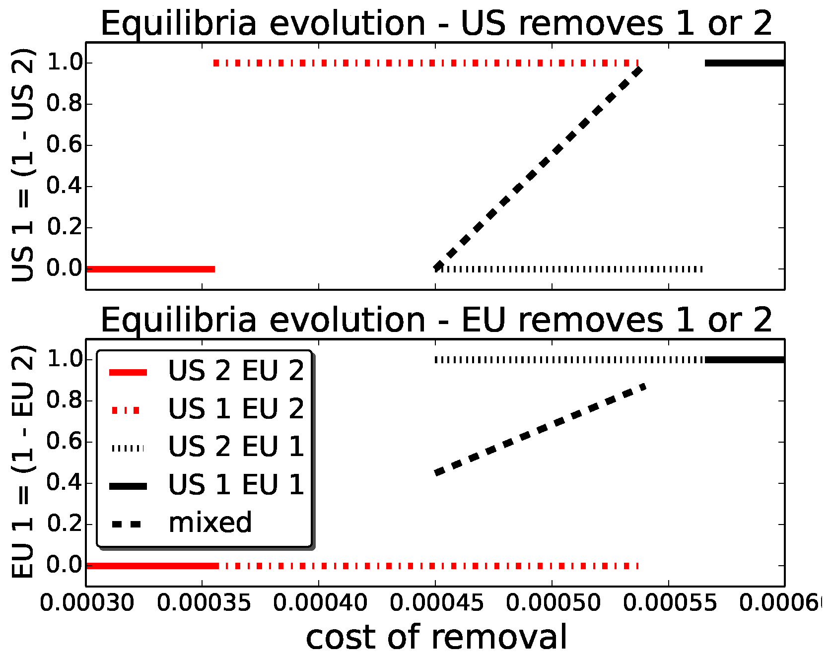
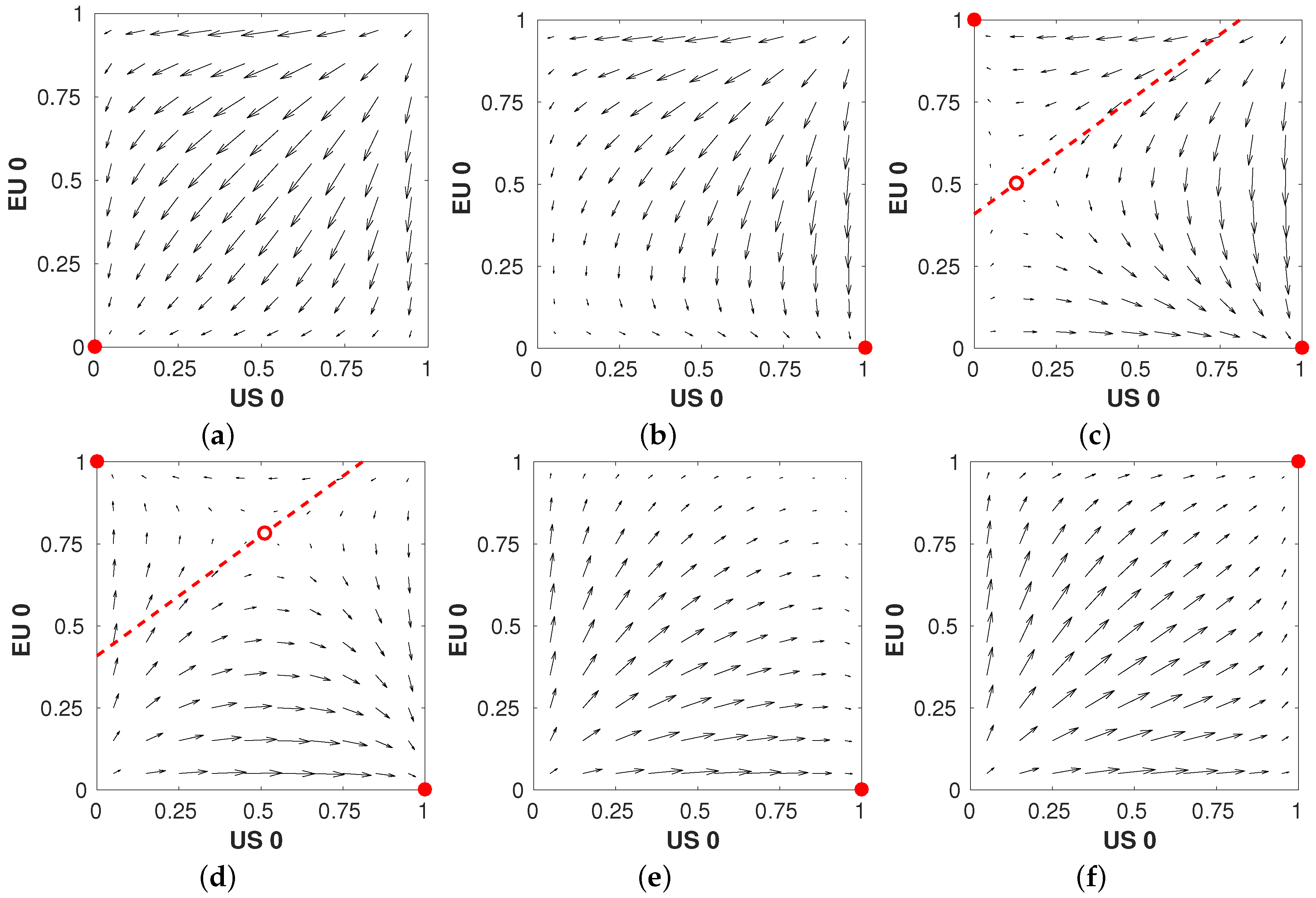
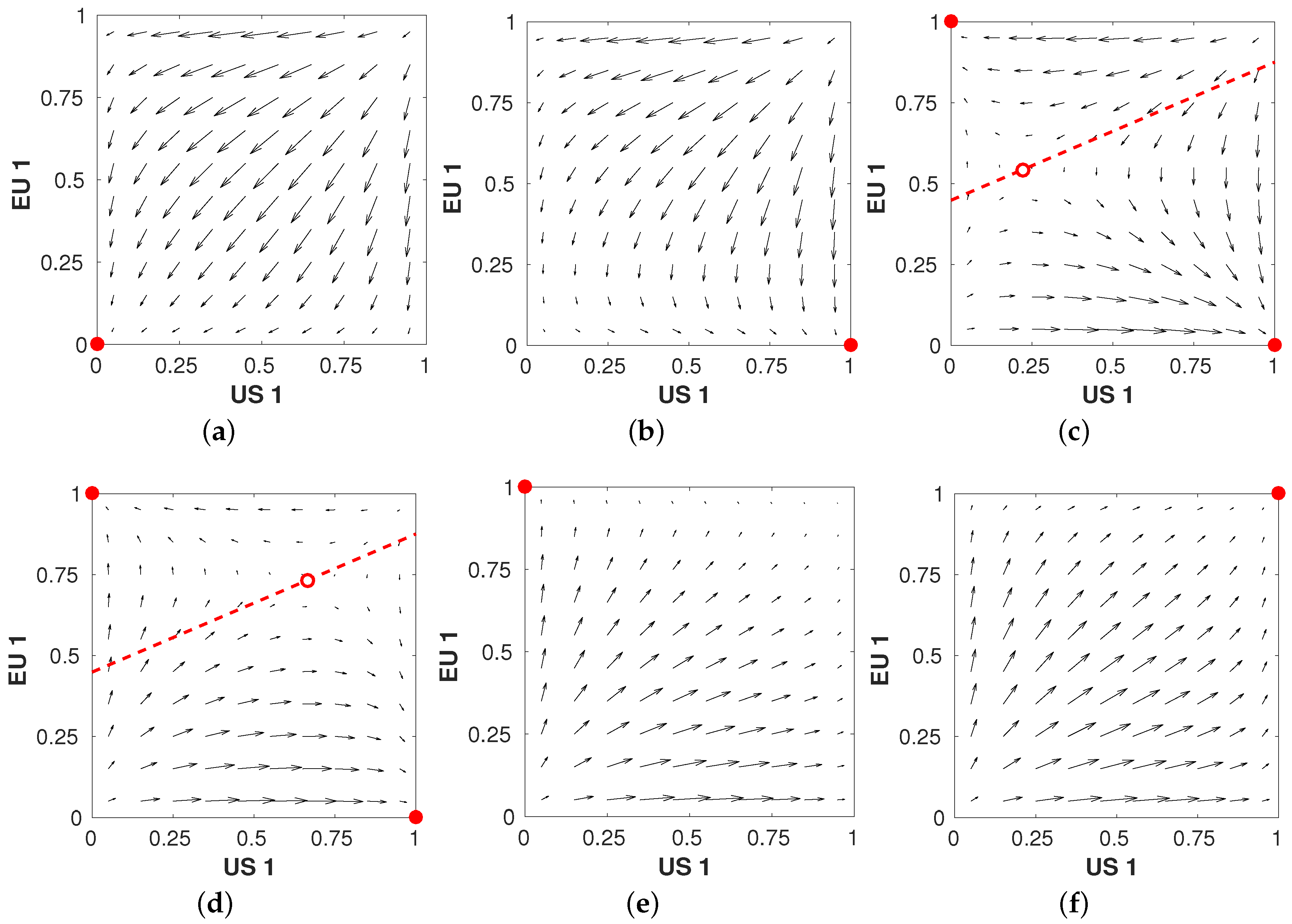
6.3. Evolutionary Dynamics

Another way to study the strategic properties of a game is by looking at the corresponding evolutionary dynamics. Evolutionary game theory 4 represents a player’s strategy by a population of individuals, each of a certain type, which corresponds to one of the player’s possible actions. The fraction of the population belonging to each type indicates the probability with which the player will play the corresponding pure action. The replicator dynamics dictate how the fraction x i of each type i in the population x changes over time due to evolutionary pressure:
x ˙ i = x i [ f i ( x ) f ¯ ( x ) ]
where f i ( x ) is the fitness (expected payoff) to type (action) i in the population and f ¯ ( x ) is the weighted average fitness of the whole population. Under the replicator dynamics, types that do better than average will increase in abundance, whereas types that do worse will decline.
Figure 9 shows the directional field of the replicator dynamics for the sub-game {remove 0, remove 1} for different values of C r corresponding to the different sets of equilibria observed in Figure 7.
The axes show the probability with which both players play the action “remove zero” (U.S. zero and EU zero). The arrows indicate the direction and magnitude of change. The replicator dynamics give insight into the stability of the different equilibria and their corresponding basins of attraction. We can conclude that the mixed Nash equilibria in Panels (c) and (d) are unstable, as a small perturbation will cause the population to move towards one of the stable pure equilibria. Moreover, we can see that the basin of attraction for the pure equilibrium {U.S. 0, EU 1} (bottom right corner) is larger than for {U.S. 1, EU 0}, indicating that this equilibrium is more likely to arise when both players iteratively optimise their strategy. This is of particular interest when full knowledge of the game is not available and the players need to learn by interacting, e.g., when space agencies mutually adapt their policy based on an estimate of other agencies’ policies. In fact, the replicator dynamics are descriptive of various multi-agent learning processes, and as such, studying these dynamics provides valuable insights in the context of adaptive agents, as well [38].
Figure 10 shows similar results for the sub-game {remove 1, remove 2}, corresponding to the different sets of equilibria observed in Figure 8. Again, we observe the instability of mixed equilibria and the differently-sized basins of attraction showing asymmetry in the game’s payoff structure.

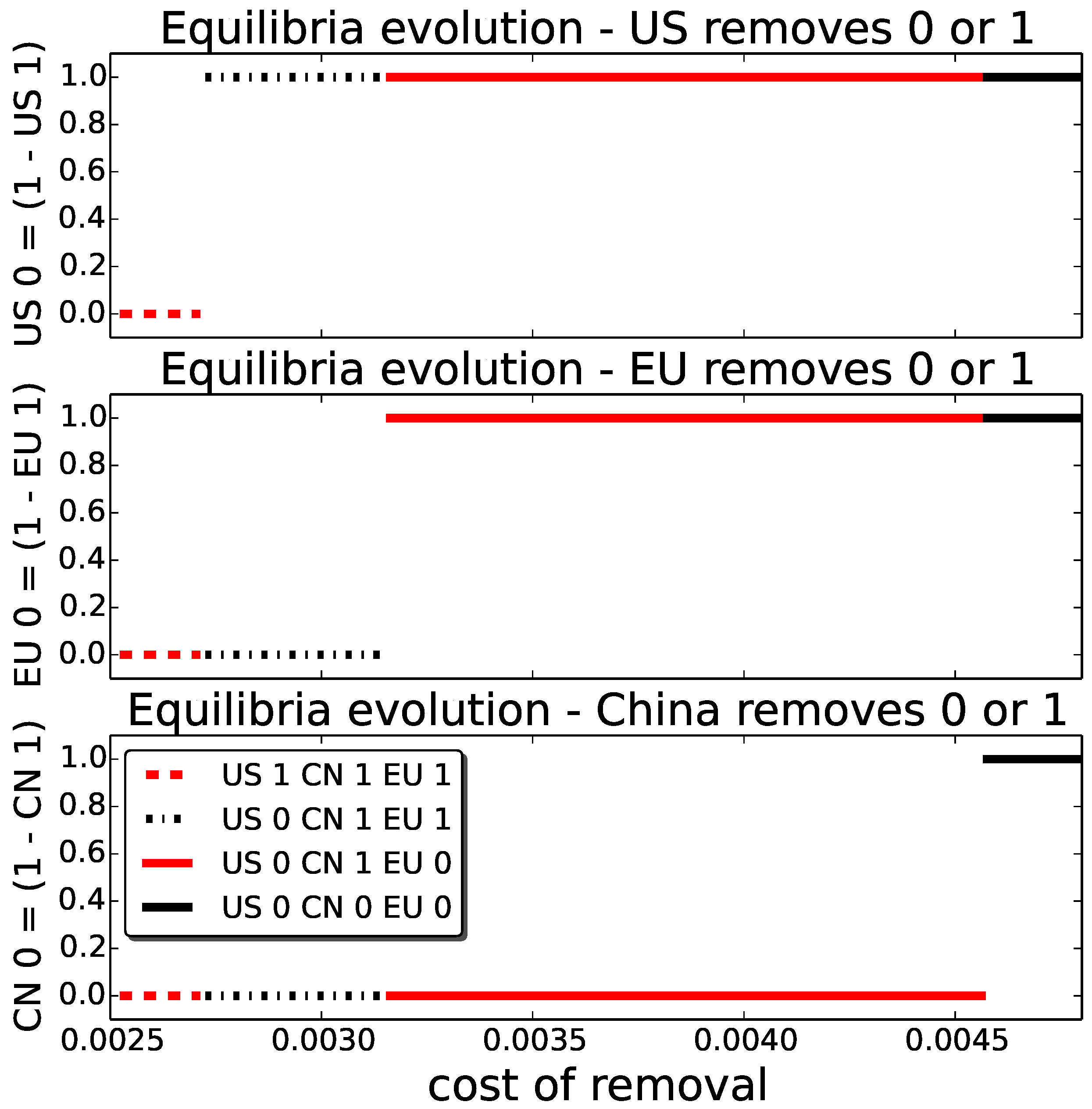
6.4. Three-Player Game

So far, we have only considered two active players. Here, we take a first step in analysing a larger game between three players (agencies): the U.S., the EU and China (CN). We focus on the two-action sub-game {remove 0, remove 1} only to facilitate analysis. Table 4 shows the cumulative risks for all three players, averaged over 180 Monte Carlo runs, as well as the corresponding confidence intervals. The risks for each player are distinguished by different font styles. We can see that the risks for China are considerably higher than for the U.S. or the EU, even though their total number of important assets is lower (see Figure 3). This interesting result may be due to the specific orbits used by each of the players, some being more dense in terms of debris than others, which requires further investigation.
At the left part of the figure, the cost of removal is low, and therefore, it is in the best interest of all three players to remove debris. However, for increasing costs, it becomes the best response for the U.S. to stop removing, and there exists a pure equilibrium (U.S. 0, EU 1, CN 1). The reason that the U.S. opts out first is due to their lower overall risk compared to the two other players. In contrast, the higher risks to China mean it is in their interest to keep removing, even when both the U.S. and EU have opted out. When the cost rises even further (the right side of the figure), we see that for none of the players removing is viable.
Although for most removal costs C r , the strategic substitute property discussed previously holds, there is a range of costs for which the property is violated. However, the payoff differences leading to this violation are not statistically significant and may be resolved by increasing the number of Monte Carlo samples of our simulation, which is left for the future work.
We can again convert the risk matrix into a payoff matrix using the payoff functions defined in Table 1. In Figure 11, we visualise the Nash equilibria for the varying costs of removal C r .

7. Conclusions and Future Work

In this paper, we have presented a new approach to study space debris removal, by introducing a multi-player non-cooperative game named the space debris removal dilemma. We implemented a realistic model of the Earth orbit environment, where we projected new future launches, collisions of space objects and natural decay for the next 150 years, for different debris removal strategies. Our experiments confirmed the commonly-predicted exponential growth of space debris in near Earth orbits. This is an important motivation to come up with mitigation strategies, such as active object removal.
In our game-theoretical analysis of this game, we identified Nash equilibria for different levels of the cost of removals; although the costs of active debris removal are still prohibitively high at the moment, they are expected to decrease with future technological development. Additionally, we investigated the strategic substitute property that appears in this type of game scenario and that guarantees the existence of a pure equilibrium under certain conditions. Although a mixed equilibrium exists for some costs, as well, it is often more desirable to focus on pure equilibria. Specifically, in our scenario, it cannot be expected that space agencies will randomize over pure strategies to decide on their space debris removal policy. Another disadvantage of a mixed equilibrium in this game is its instability (as shown in Figure 9), which is undesirable in our scenario, where the choice of action taken has a huge impact on the Earth orbit environment. The results of this study help agencies to better understand the debris removal problem, and its short- and long-term consequences, in order to prepare for mitigation strategies. For instance, we show that removing just one high risk debris object every two years can already substantially decrease the risk of collision for active satellites. Additionally, the removal of indirect collision risks is beneficial, as well as it reduces the number of potential future on-orbit collisions.
There are many routes for future work. Projecting the future evolution of space debris itself is a very complex problem with many unknown variables and inputs, and therefore, some necessary simplifications and assumptions have been made. Despite these simplifications, the simulation is computationally demanding, which makes it difficult to obtain the necessary number of Monte Carlo runs, especially for larger games. In future work, we aim to use HPC clusters to obtain statistically-significant results for more extensive scenarios, in which we can include more players (e.g., Russia, India), as well as more diverse debris removal strategies. For example, different types of removal missions may come with different associated cost and success rates, which could further enrich the strategic aspects of the model.
From a game-theoretic point of view, our approach has been limited to a one-shot normal-form game, which assumes that agencies fix their removal policy for the entire time horizon up front. More realistically, these strategies may be adaptive and dependent on the state of the LEO environment, as well as on current and past actions by others. One possible future direction is to move to the framework of stochastic or dynamic games. Finally, the strategic substitutes property can be further investigated, for example by attempting to fit a parametrised game to the empirical results. If successful, this would greatly reduce the computational burden of running a variety of similar experiments.

Acknowledgments

This work was supported by the European Space Agency under the Ariadna initiative, Study Reference No. 15/8401.

Author Contributions

All authors contributed equally to the conception and design of the experiments. R.K. throughout performed the experiments and analysed the data. D.B., R.S. and K.T. contributed to the game theoretic analysis. D.H. and D.I. provided input on space debris and active debris removal. All authors wrote the paper.

Conflicts of Interest

The authors declare no conflict of interest.

References

  1. NORAD Two-Line Element Sets Current Data. Available online: https://celestrak.com/NORAD/elements/ (accessed on 1 February 2016).
  2. Carrico, T.; Carrico, J.; Policastri, L.; Loucks, M. Investigating orbital debris events using numerical methods with full force model orbit propagation. Adv. Astronaut. Sci. 2008, 130, 407–426. [Google Scholar]
  3. NASA Orbital Debris Program Office. Chinese Anti-Satellite Test Creates Most Severe Orbital Debris Cloud in History. In NASA Orbital Debris Quarterly News; NASA Orbital Debris Program Office: Houston, TX, USA, 2007. [Google Scholar]
  4. NASA Orbital Debris Program Office. Satellite Collision Leaves Significant Debris Clouds. In NASA Orbital Debris Quarterly News; NASA Orbital Debris Program Office: Houston, TX, USA, 2009. [Google Scholar]
  5. NASA Orbital Debris Program Office. International Space Station Again Dodges Debris. In NASA Orbital Debris Quarterly News; NASA Orbital Debris Program Office: Houston, TX, USA, 2011. [Google Scholar]
  6. Tahvonen, O. Carbon dioxide abatement as a differential game. Eur. J. Polit. Econ. 1994, 10, 685–705. [Google Scholar] [CrossRef]
  7. Kessler, D.J.; Cour-Palais, B.G. Collision frequency of artificial satellites: The creation of a Debris belt. J. Geophys. Res. 1978, 83, 2637–2646. [Google Scholar] [CrossRef]
  8. Kessler, D.J.; Johnson, N.L.; Liou, J.C.; Matney, M. The Kessler syndrome: Implications to future space operations. In Proceedings of the American Astronautical Society—Guidance Control Conference, Breckenridge, CO, USA, 6–10 February 2010.
  9. Liou, J.C.; Johnson, N.L. A sensitivity study of the effectiveness of active debris removal in LEO. Acta Astronaut. 2009, 64, 236–243. [Google Scholar] [CrossRef]
  10. Liou, J.C.; Johnson, N.L.; Hill, N. Controlling the growth of future LEO debris populations with active debris removal. Acta Astronaut. 2010, 66, 648–653. [Google Scholar] [CrossRef]
  11. Liou, J.C. An active debris removal parametric study for LEO environment remediation. Adv. Space Res. 2011, 47, 1865–1876. [Google Scholar] [CrossRef]
  12. Harstad, B. Climate contracts: A game of emissions, investments, negotiations, and renegotiations. Rev. Econ. Stud. 2012, 79, 1527–1557. [Google Scholar] [CrossRef]
  13. Levhari, D.; Mirman, L.J. The great fish war: An example using a dynamic Cournot-Nash solution. Bell J. Econ. 1980, 11, 322–334. [Google Scholar] [CrossRef]
  14. Hardin, G. The tragedy of the commons. Science 1968, 162, 1243–1248. [Google Scholar] [CrossRef] [PubMed]
  15. Walsh, W.; Das, R.; Tesauro, G.; Kephart, J. Analyzing complex strategic interactions in multi-agent systems. In Proceedings of the AAAI-02 Workshop on Game-Theoretic and Decision-Theoretic Agents, Edmonton, AB, Canada, 28 July–1 August 2002.
  16. Wellman, M.P. Methods for empirical game-theoretic analysis. In Proceedings of the Twenty-First National Conference on Artificial Intelligence and the Eighteenth Innovative Applications of Artificial Intelligence Conference, Boston, MA, USA, 16–20 July 2006; AAAI Press: Menlo Park, CA, USA; MIT Press: Cambridge, MA, USA; London, UK, 2006; Volume 21, pp. 1552–1555. [Google Scholar]
  17. Jordan, P.R.; Vorobeychik, Y.; Wellman, M.P. Searching for approximate equilibria in empirical games. In Proceedings of the 7th International Joint Conference on Autonomous Agents and Multiagent Systems, Estoril, Portugal, 12–16 May 2008; International Foundation for Autonomous Agents and Multiagent Systems: Richland, SC, USA, 2008; Volume 2, pp. 1063–1070. [Google Scholar]
  18. Wellman, M.P.; Jordan, P.R.; Kiekintveld, C.; Miller, J.; Reeves, D.M. Empirical game-theoretic analysis of the TAC market games. In Proceedings of the AAMAS-06 Workshop on Game-Theoretic and Decision-Theoretic Agents, Hakodate, Japan, 8–10 May 2006.
  19. Phelps, S.; Parsons, S.; McBurney, P. An evolutionary game-theoretic comparison of two double-auction market designs. In Agent-Mediated Electronic Commerce VI. Theories for and Engineering of Distributed Mechanisms and Systems; Lecture Notes in Computer Science; Faratin, P., Rodríguez-Aguilar, J.A., Eds.; Springer: Berlin Germany; Heidelberg, Germany, 2005; Volume 3435, pp. 101–114. [Google Scholar]
  20. Ponsen, M.; Tuyls, K.; Kaisers, M.; Ramon, J. An evolutionary game-theoretic analysis of poker strategies. Entertain. Comput. 2009, 1, 39–45. [Google Scholar] [CrossRef]
  21. Hennes, D.; Claes, D.; Tuyls, K. Evolutionary advantage of reciprocity in collision avoidance. In Proceedings of the AAMAS 2013 Workshop on Autonomous Robots and Multirobot Systems (ARMS 2013), Saint Paul, MN, USA, 6–10 May 2013.
  22. Wellman, M.P.; Prakash, A. Empirical game-theoretic analysis of an adaptive cyber-defense scenario (preliminary report). In Proceedings of Conference on Decision and Game Theory for Security, 6–7 November 2014; pp. 43–58.
  23. Hennes, D.; Jong, S.D.; Tuyls, K.; Gal, Y.K. Metastrategies in large-scale bargaining settings. ACM Trans. Intell. Syst. Technol. (TIST) 2015, 7, 10. [Google Scholar] [CrossRef]
  24. Izzo, D. Pygmo and Pykep: Open Source Tools for Massively Parallel Optimization in Astrodynamics (The Case of Interplanetary Trajectory Optimization); Technical Report; Advanced Concept Team—European Space Research and Technology Centre (ESTEC): Noordwijk, The Netherlands, 2012. [Google Scholar]
  25. Liou, J.C.; Kessler, D.; Matney, M.; Stansbery, G. A new approach to evaluate collision probabilities among asteroids, comets, and Kuiper Belt objects. In Proceedings of the Lunar and Planetary Science Conference, League City, TX, USA, 17–21 March 2003; Volume 34, p. 1828.
  26. Vallado, D.A.; Crawford, P.; Hujsak, R.; Kelso, T. Revisiting spacetrack report #3. AIAA 2006, 6753, 2006. [Google Scholar]
  27. Johnson, N.L.; Krisko, P.H.; Liou, J.C.; Anz-Meador, P.D. Nasa’s new breakup model of EVOLVE 4.0. Adv. Space Res. 2001, 28, 1377–1384. [Google Scholar] [CrossRef]
  28. Klinkrad, H. Space Debris. In Encyclopedia of Aerospace Engineering; The American Institute of Aeronautics and Astronautics: Reston, VA, USA, 2010. [Google Scholar]
  29. Gibbons, R. A Primer in Game Theory; Financial Times Prentice Hall, Pearson Education: Harlow, Essex, UK, 1992. [Google Scholar]
  30. Nash, J. Non-cooperative games. Ann. Math. 1951, 54, 286–295. [Google Scholar] [CrossRef]
  31. Novshek, W. On the existence of Cournot equilibrium. Rev. Econ. Stud. 1985, 52, 85–98. [Google Scholar] [CrossRef]
  32. Rodrigo Bamón, J.F. Existence of Cournot equilibrium in large markets. Econometrica 1985, 53, 587–597. [Google Scholar]
  33. Dubey, P.; Haimanko, O.; Zapechelnyuk, A. Strategic complements and substitutes, and potential games. Games Econ. Behav. 2006, 54, 77–94. [Google Scholar] [CrossRef]
  34. Kukushkin, N.S. Best response dynamics in finite games with additive aggregation. Games Econ. Behav. 2004, 48, 94–110. [Google Scholar] [CrossRef]
  35. Kukushkin, N.S. A fixed-point theorem for decreasing mappings. Econ. Lett. 1994, 46, 23–26. [Google Scholar] [CrossRef]
  36. Kukushkin, N.S. Strategic supplements in games with polylinear interactions. Available online: http://www.eco.uc3m.es/temp/StrSuppl.pdf (accessed on 6 April 2016).
  37. Weibull, J.W. Evolutionary Game Theory; MIT Press: Cambridge, MA, USA, 1997. [Google Scholar]
  38. Bloembergen, D.; Tuyls, K.; Hennes, D.; Kaisers, M. Evolutionary dynamics of multi-agent learning: A survey. J. Artif. Intell. Res. 2015, 53, 659–697. [Google Scholar]
Figure 1. Orbital inclination distribution.
Games 07 00020 g001
Figure 2. Spatial density prediction in Low Earth Orbit (LEO).
Games 07 00020 g002
Figure 3. Important assets’ development.
Games 07 00020 g003
Figure 4. Debris evolution for next 150 years.
Games 07 00020 g004
Figure 5. Evolution of overall risk to important assets for different combinations of actions of both the U.S. and EU. (a) Risk to U.S. assets; (b) risk to EU assets.
Games 07 00020 g005
Figure 6. Free-riding effect in the overall risk to important assets for non-active players China and Russia, for combinations of actions of both the U.S. and EU. (a) Risk to Chinese assets; (b) risk to Russian assets.
Games 07 00020 g006
Figure 7. Equilibrium strategies for the sub-game {remove 0, remove 1} for a range of removal costs C r .
Games 07 00020 g007
Figure 8. Equilibrium strategies for the sub-game {remove 1, remove 2} for a range of removal costs C r .
Games 07 00020 g008
Figure 9. Evolutionary dynamics of the sub-game {remove 0, remove 1} for different values of C r . Stable attractors are indicated with and unstable attractors with . The dotted line indicates the trajectory on which the mixed equilibrium moves as C r changes. (a) C r = 0 . 0024 ; (b) C r = 0 . 0027 ; (c) C r = 0 . 00285 ; (d) C r = 0 . 003 ; (e) C r = 0 . 00315 ; (f) C r = 0 . 0033 .
Games 07 00020 g009
Figure 10. Evolutionary dynamics of the subgame { remove 1 , remove 2 } for different values of C r . Stable attractors are indicated with and unstable attractors with . The dotted line indicates the trajectory on which the mixed equilibrium moves as C r changes. (a) C r = 0 . 0003 ; (b) C r = 0 . 0004 ; (c) C r = 0 . 00047 ; (d) C r = 0 . 00051 ; (e) C r = 0 . 00055 ; (f) C r = 0 . 0006 .
Games 07 00020 g010
Figure 11. U.S., EU and China equilibria for different costs of removal.
Games 07 00020 g011
Table 1. Payoff functions for the different strategies.
StrategyPayoff Function
Remove 2 ( r · C l + T · C r )
Remove 1 ( r · C l + 0 . 5 · T · C r )
Remove 0 ( r · C l )
Table 2. Risk matrix for both players for each combination of strategies. The risks are the average cumulative risk of losing an asset over the course of 150 years. We show 95% confidence intervals in the lower table.
EU 2EU 1EU 0
U.S. 2 0 . 03413 , 0 . 03733 0 . 05247 , 0 . 07108 0 . 07704 , 0 . 27474
U.S. 1 0 . 06073 , 0 . 06352 0 . 09499 , 0 . 10405 0 . 10885 , 0 . 31401
U.S. 0 0 . 25022 , 0 . 07368 0 . 28848 , 0 . 12447 0 . 34261 , 0 . 36385
U.S. 2 ± 0 . 00528 , ± 0 . 00563 ± 0 . 00712 , ± 0 . 00785 ± 0 . 00838 , ± 0 . 01874
U.S. 1 ± 0 . 00689 , ± 0 . 00767 ± 0 . 00820 , ± 0 . 00938 ± 0 . 00994 , ± 0 . 01954
U.S. 0 ± 0 . 01896 , ± 0 . 00786 ± 0 . 01685 , ± 0 . 01061 ± 0 . 01831 , ± 0 . 01859
Table 3. Payoff matrix for both players for each combination of strategies for C r = 0 . 003 .
EU 2EU 1EU 0
U.S. 2 0 . 48413 , 0 . 48733 0 . 50247 , 0 . 29608 0 . 52704 , 0 . 27474
U.S. 1 0 . 28573 , 0 . 51352 0 . 31999 , 0 . 32905 0 . 33385 , 0 . 31401
U.S. 0 0 . 25022 , 0 . 52368 0 . 28848 , 0 . 34947 0 . 34261 , 0 . 36385
Table 4. Risk matrix (top) and corresponding 95% confidence intervals (bottom) for a three-player two-action game. Players are the U.S., EU and China, the font type shows risk values belonging to each player.
EU 1EU 0
CN 1U.S. 1 0 . 07013 , 0 . 08621 , 0 . 10162 0 . 09185 , 0 . 31547 , 0 . 13320
U.S. 0 0 . 27373 , 0 . 10294 , 0 . 12226 0 . 30759 , 0 . 33980 , 0 . 15468
CN 0U.S. 1 0 . 09229 , 0 . 10067 , 0 . 38774 0 . 11226 , 0 . 32031 , 0 . 43121
U.S. 0 0 . 28510 , 0 . 12539 , 0 . 43225 0 . 34400 , 0 . 36335 , 0 . 49774
CN 1U.S. 1 ± 0 . 0061 , ± 0 . 0074 , ± 0 . 0086 ± 0 . 0071 , ± 0 . 0174 , ± 0 . 0103
U.S. 0 ± 0 . 0163 , ± 0 . 0080 , ± 0 . 0098 ± 0 . 0184 , ± 0 . 0189 , ± 0 . 0110
CN 0U.S. 1 ± 0 . 0077 , ± 0 . 0087 , ± 0 . 0255 ± 0 . 0093 , ± 0 . 0183 , ± 0 . 0260
U.S. 0 ± 0 . 0157 , ± 0 . 0099 , ± 0 . 0275 ± 0 . 0181 , ± 0 . 0180 , ± 0 . 0279

