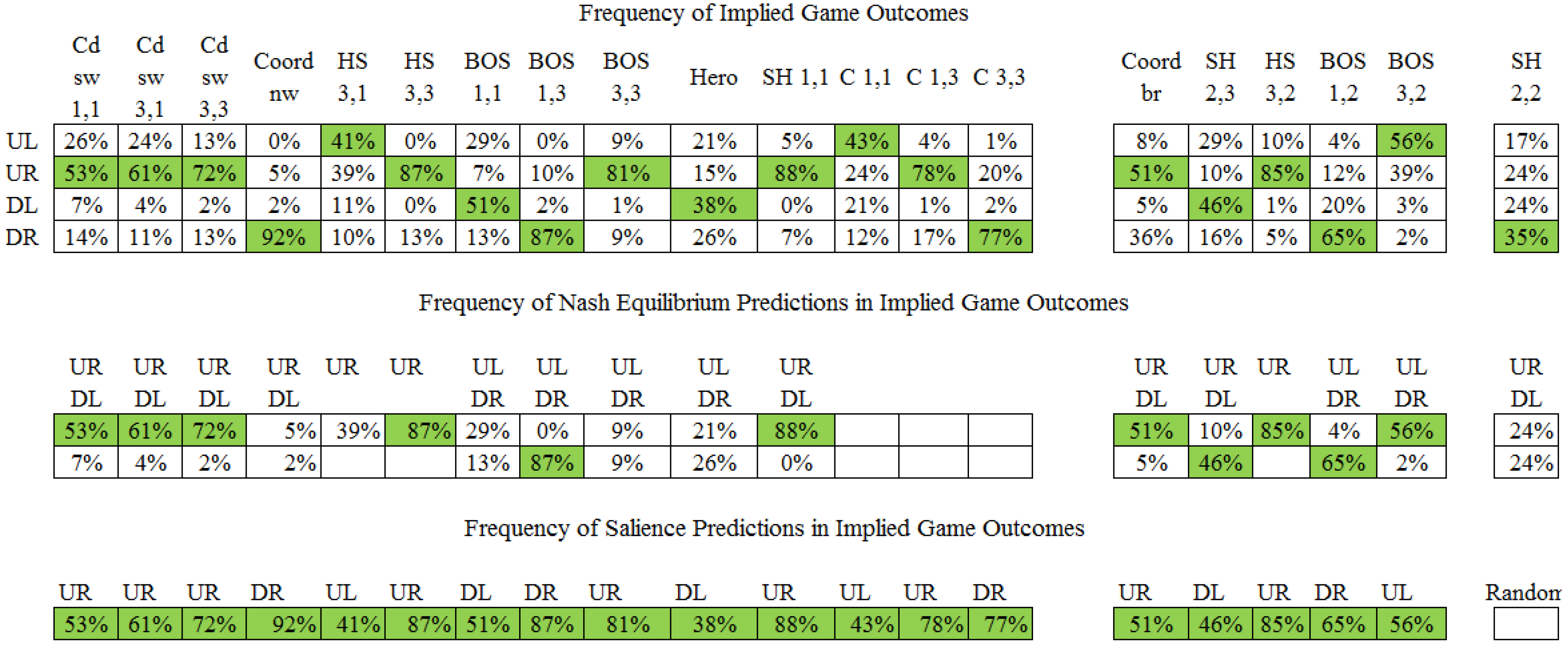
For the purposes of examining the implications of salience in games, we begin by defining those payoffs in the game that are perceived as salient by a player.
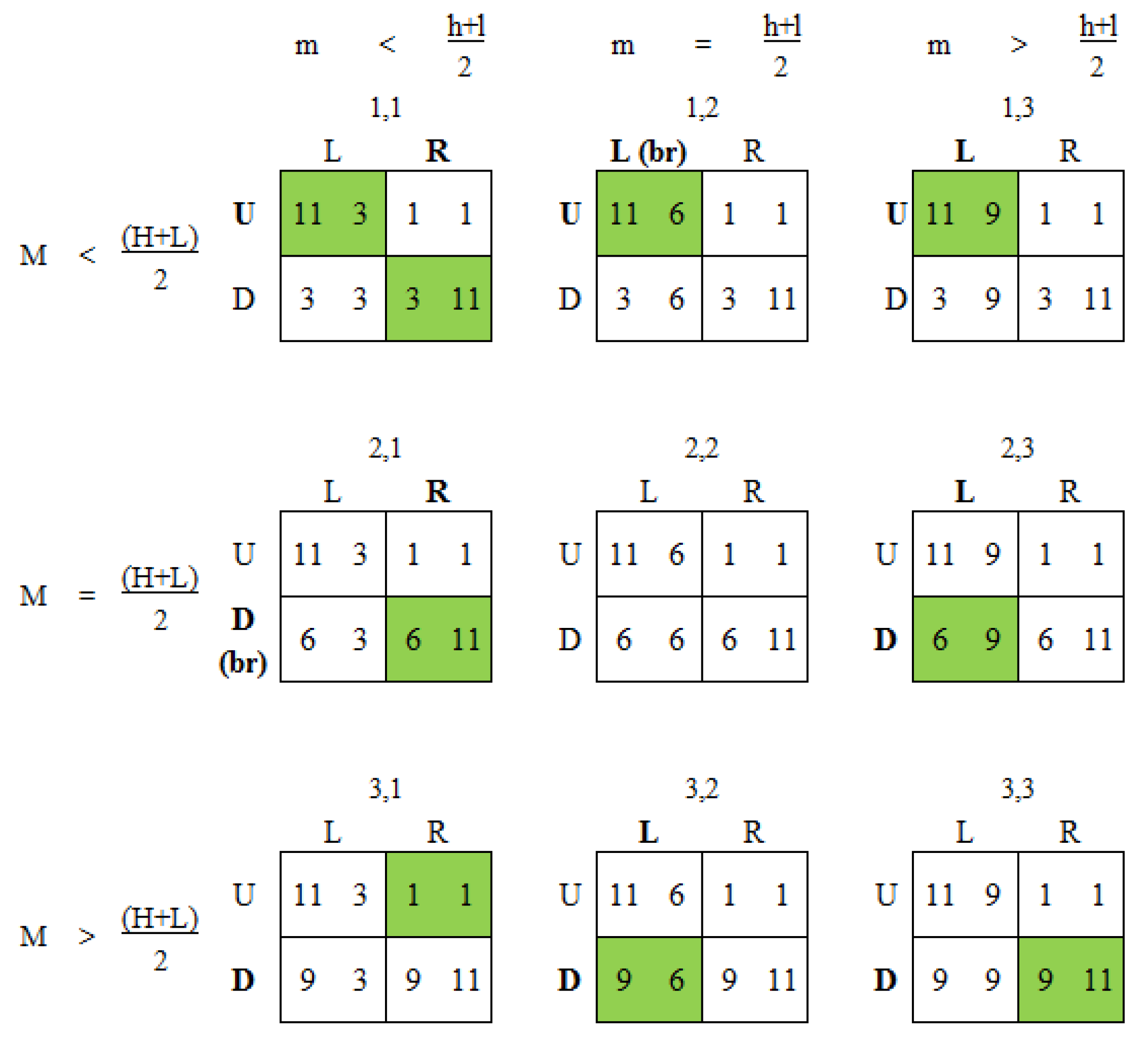
When the difference in payoffs to P1 from choosing U or D, conditional on P2 choosing L, are not equal to the difference in payoffs to P1, conditional on P2 choosing R, only those payoffs to P1 associated with the larger difference are perceived as salient. When the differences are equal and of the same or opposite sign, no payoffs are perceived as more salient than the others.
2.1. Implications of Own-Payoff Salience
Depending on whether there are ties in the payoffs of one or both players and whether the identity of the players is viewed as important there are between 78 [
24] and 1431 [
25,
26] unique 2 × 2 games. In a compromise between completeness and brevity, we will focus our discussion on Robinson and Goforth’s [
27] typology of 144 strictly ordinal games, depicted in blocks of 36 games in
Figure 2,
Figure 3,
Figure 4 and
Figure 5. A bird’s eye view of the entire set is provided in
Figure A1 in the appendix.
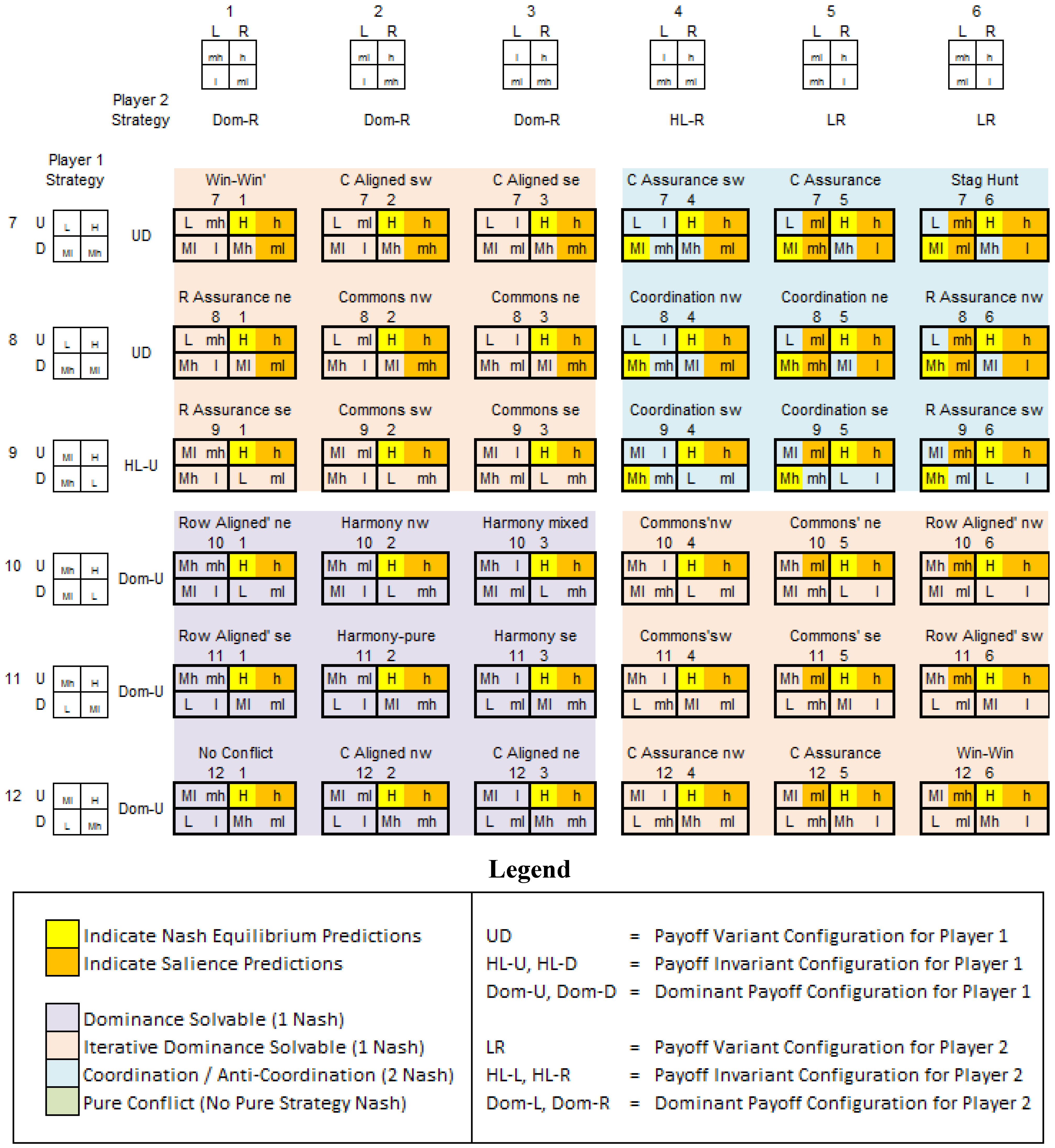
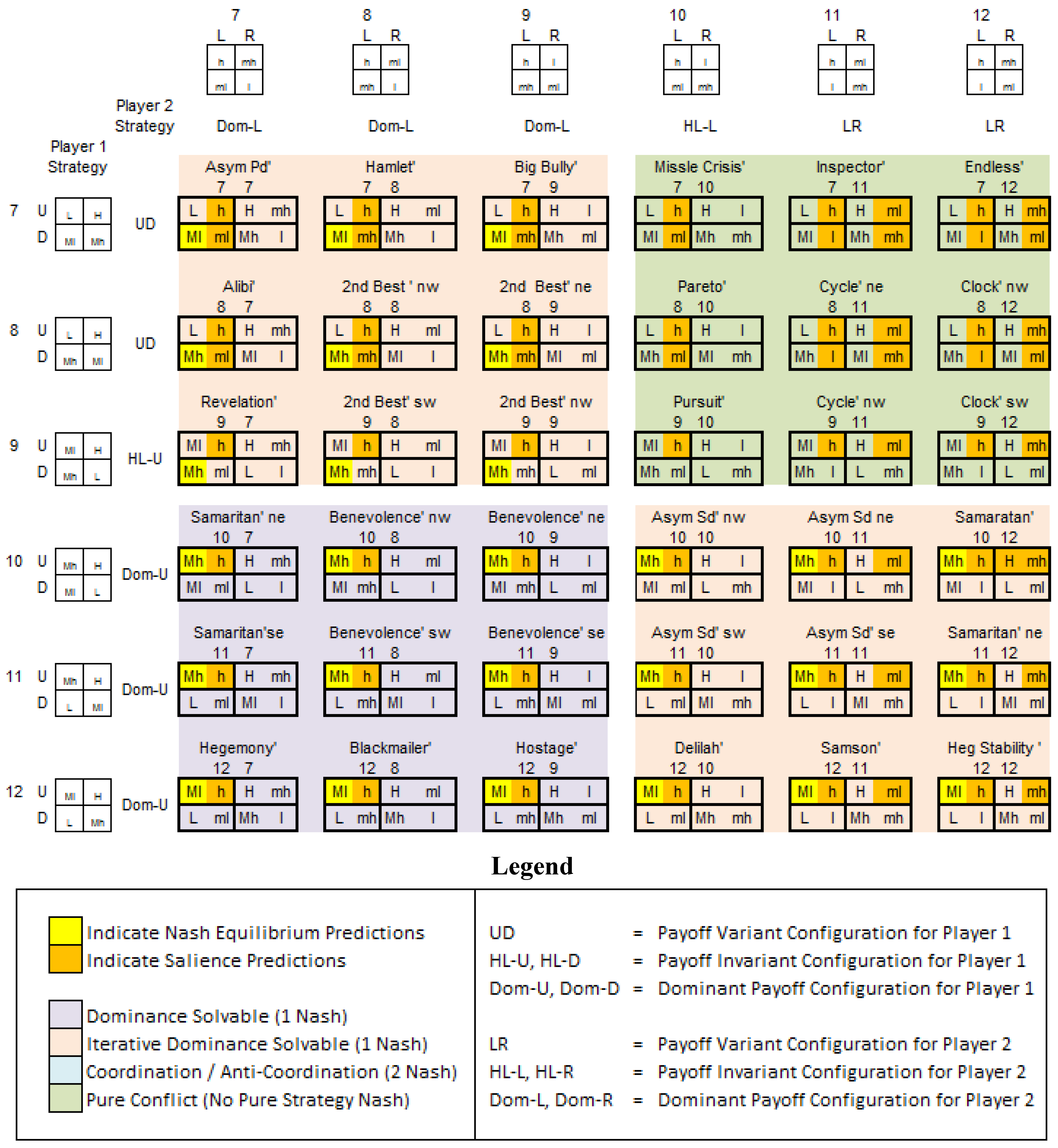
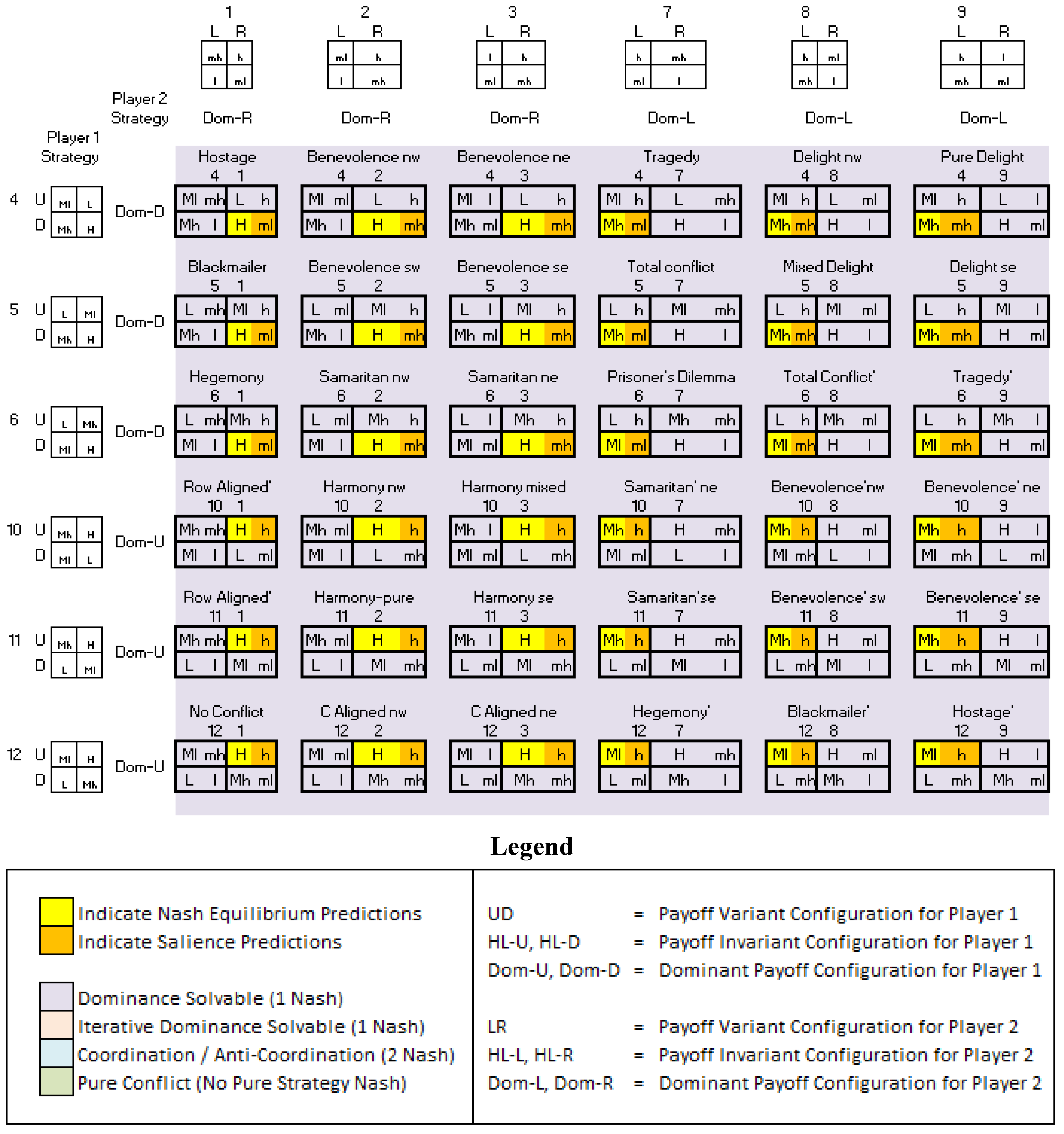
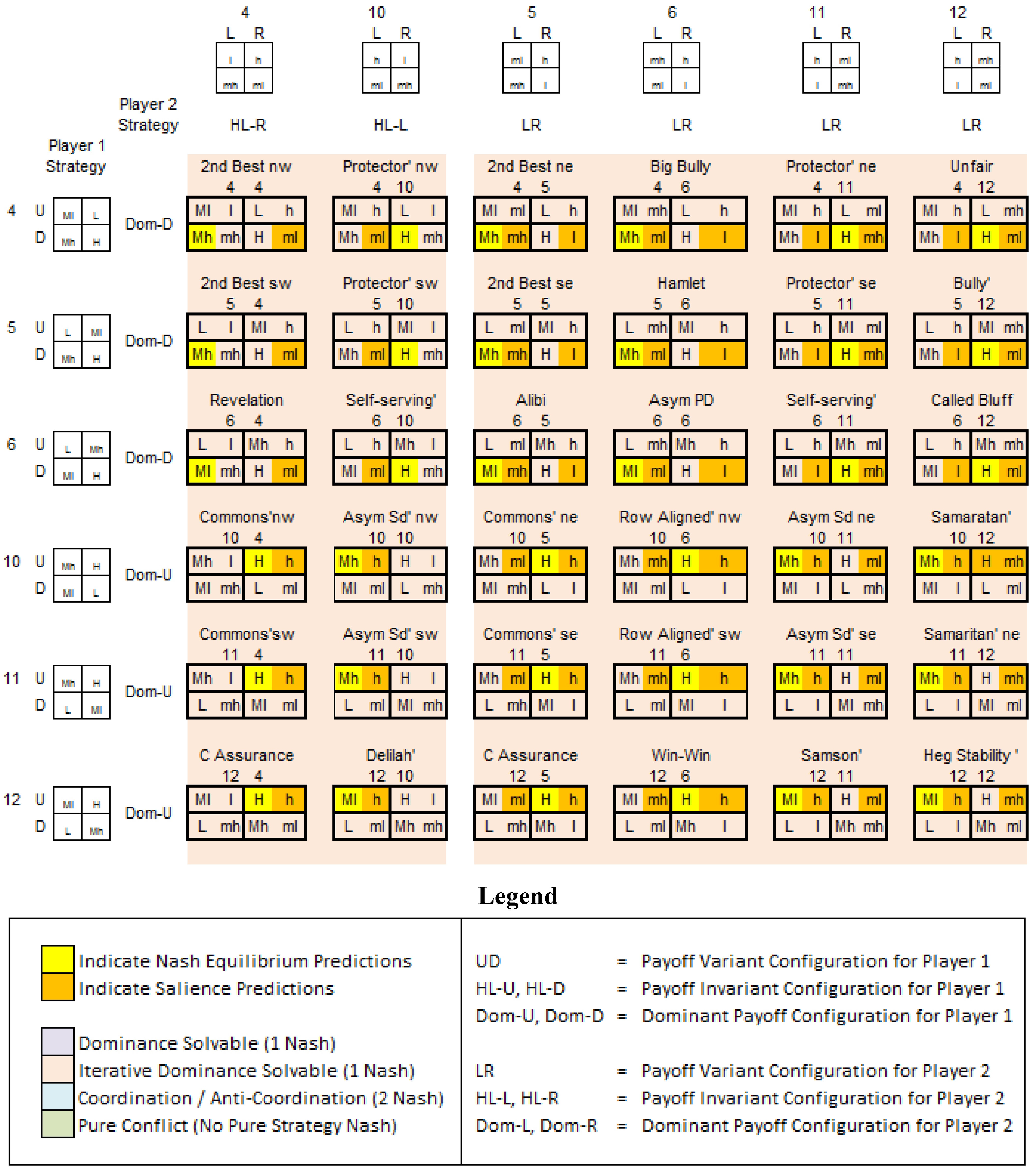
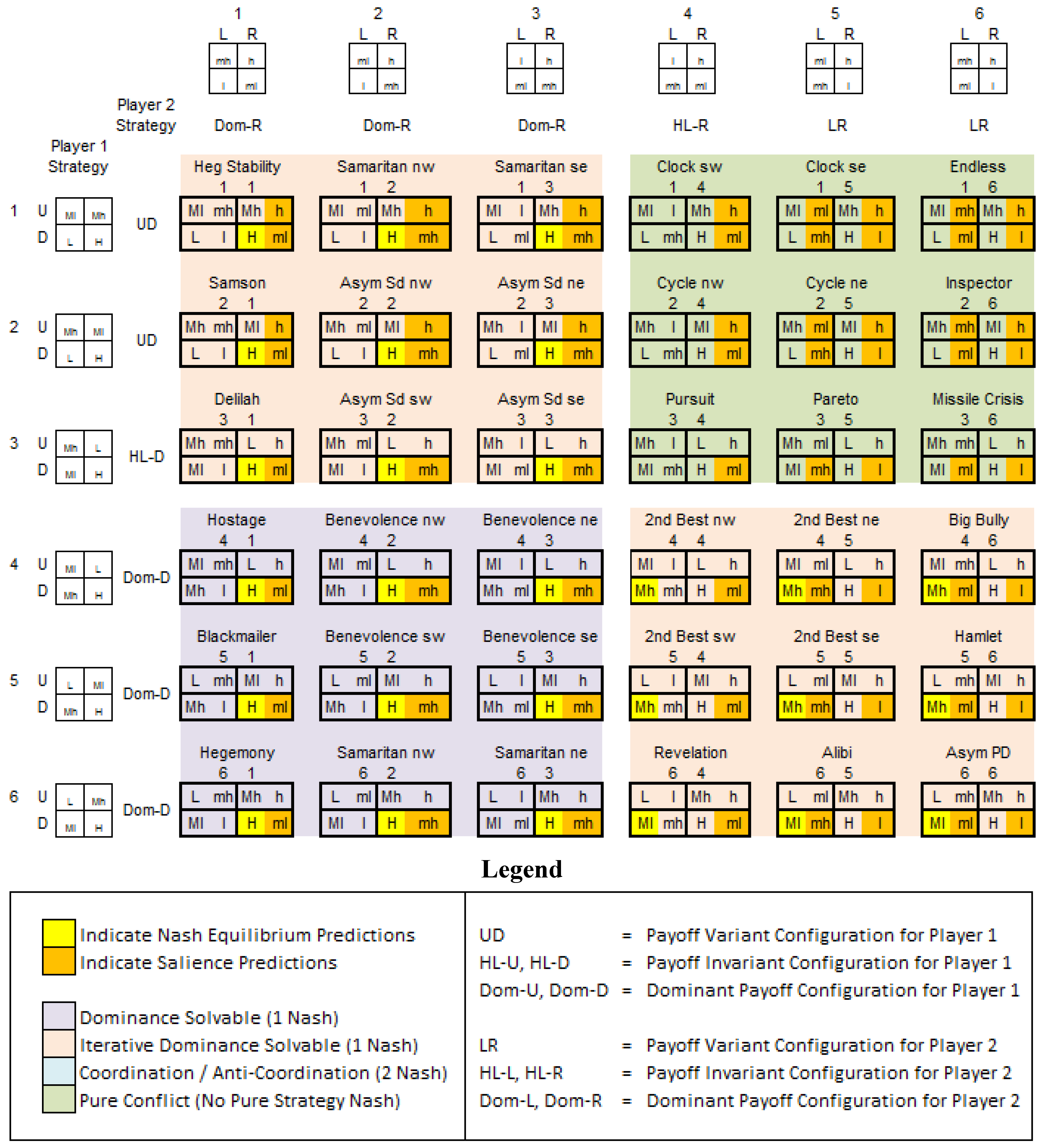
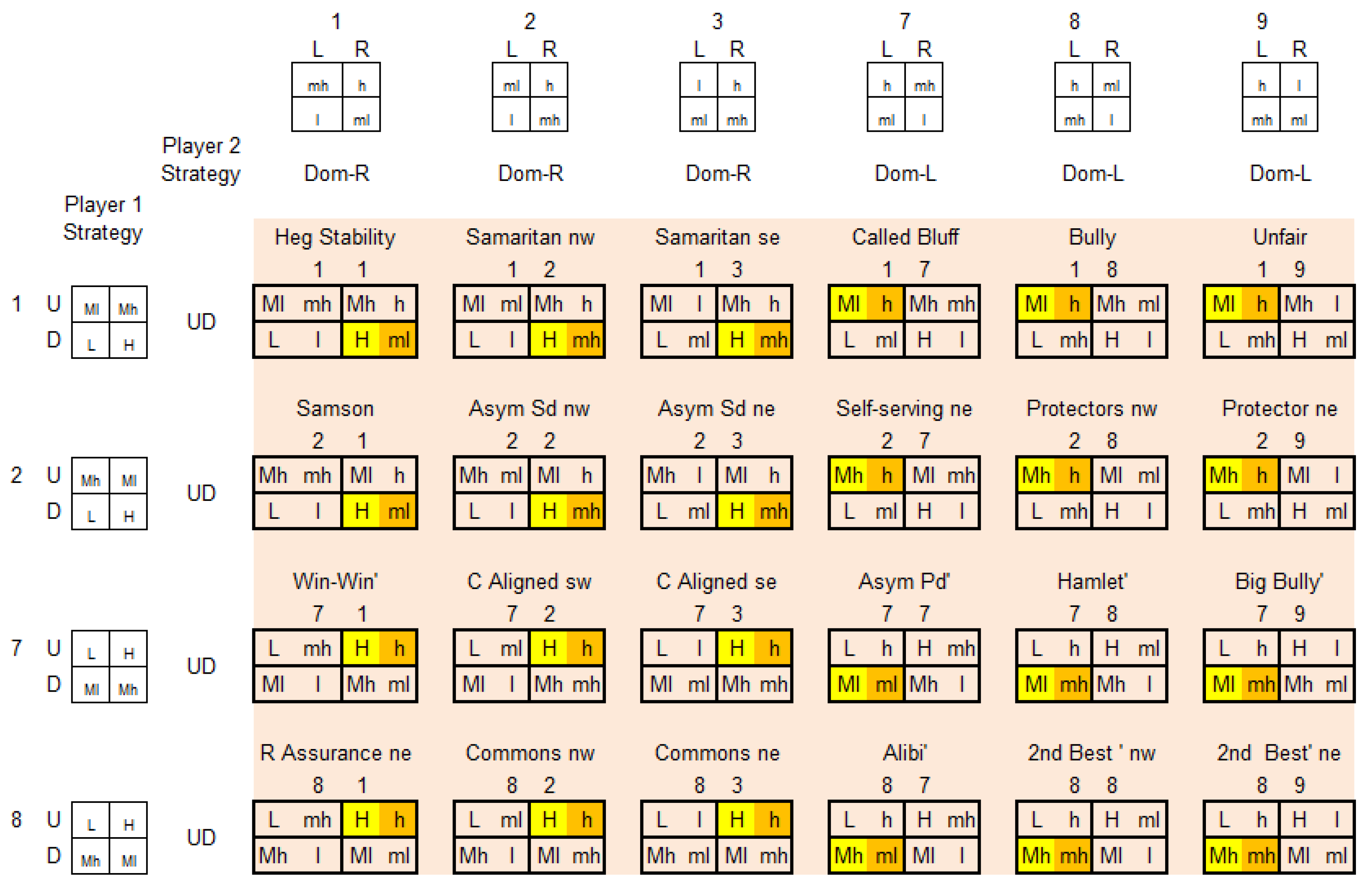
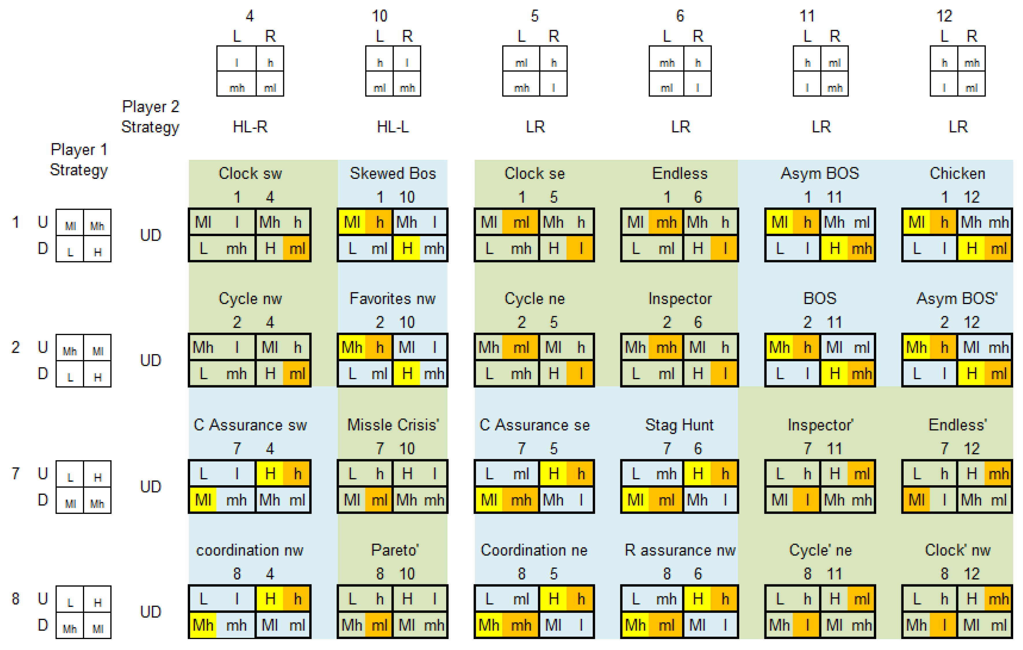
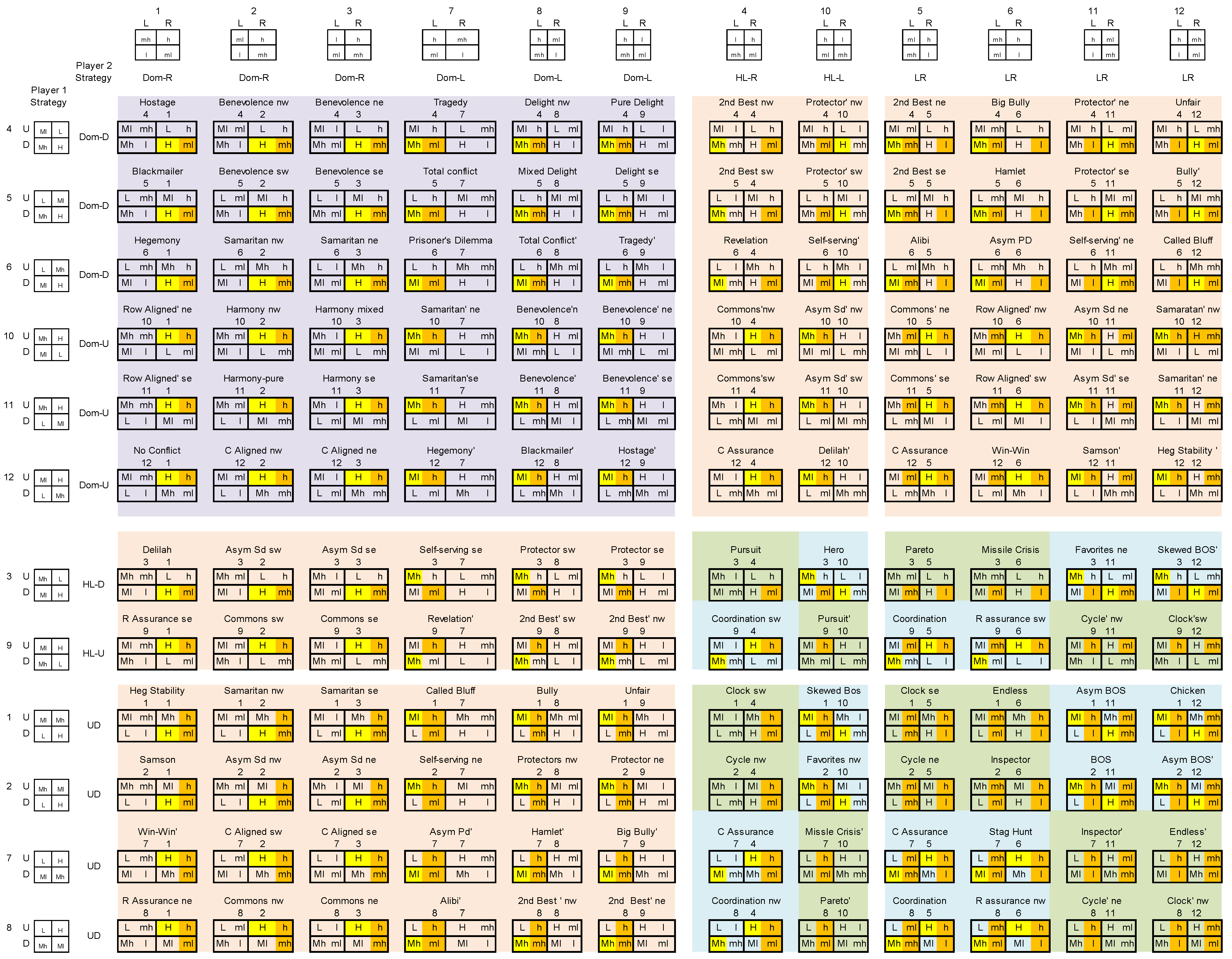
In Robinson and Goforth’s typology there are 12 possible payoff structures for each player. For six of these, there is a dominating strategy so 36 of the games are solved by dominance. The games where both players have dominating strategies are the ones clustered in purple. According to game theory, the outcome in these will be the dominating Nash equilibrium (where here and throughout the figures in
Section 2, Nash equilibria are indicated by yellow cells containing a payoff in bold.) An additional 72 games are dominance solvable—one player has a dominating strategy and the other best responds. These are the clusters of games shaded in beige. The two clusters of games in blue involve payoff configurations that produce coordination and anti-coordination games, respectively. For these games, traditional game theory predicts that one of the two Nash outcomes will obtain but does not specify which will occur. Finally, there are two clusters of games in green. These are cyclic games for which game theory makes no pure strategy predictions.
Figure 2.
The class of 144 strictly ordinal 2 × 2 games (games 1–1 through 6–6).
Figure 2.
The class of 144 strictly ordinal 2 × 2 games (games 1–1 through 6–6).
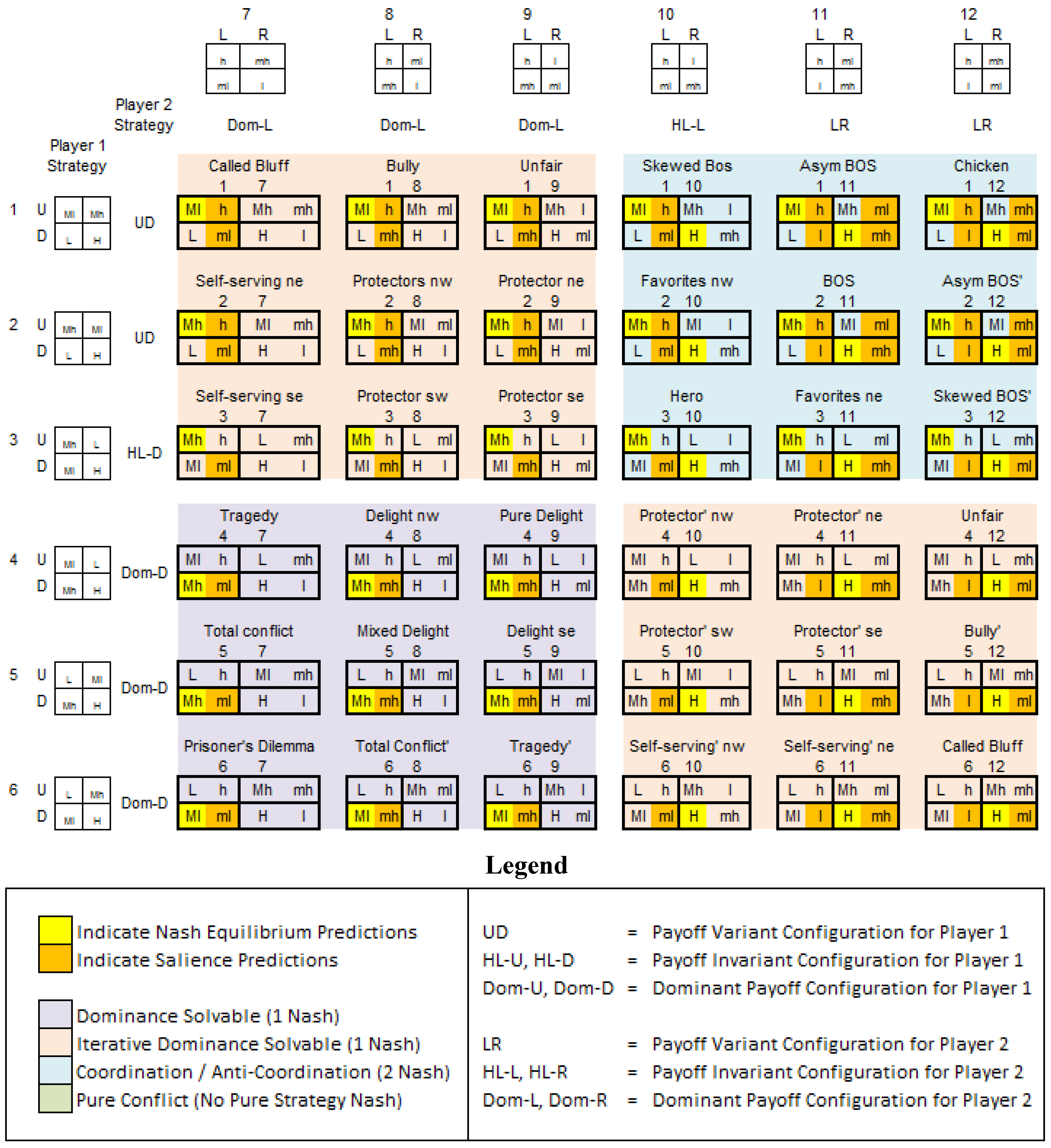
Figure 3.
The class of 144 strictly ordinal 2 × 2 games (games 1–7 through 6–12).
Figure 3.
The class of 144 strictly ordinal 2 × 2 games (games 1–7 through 6–12).
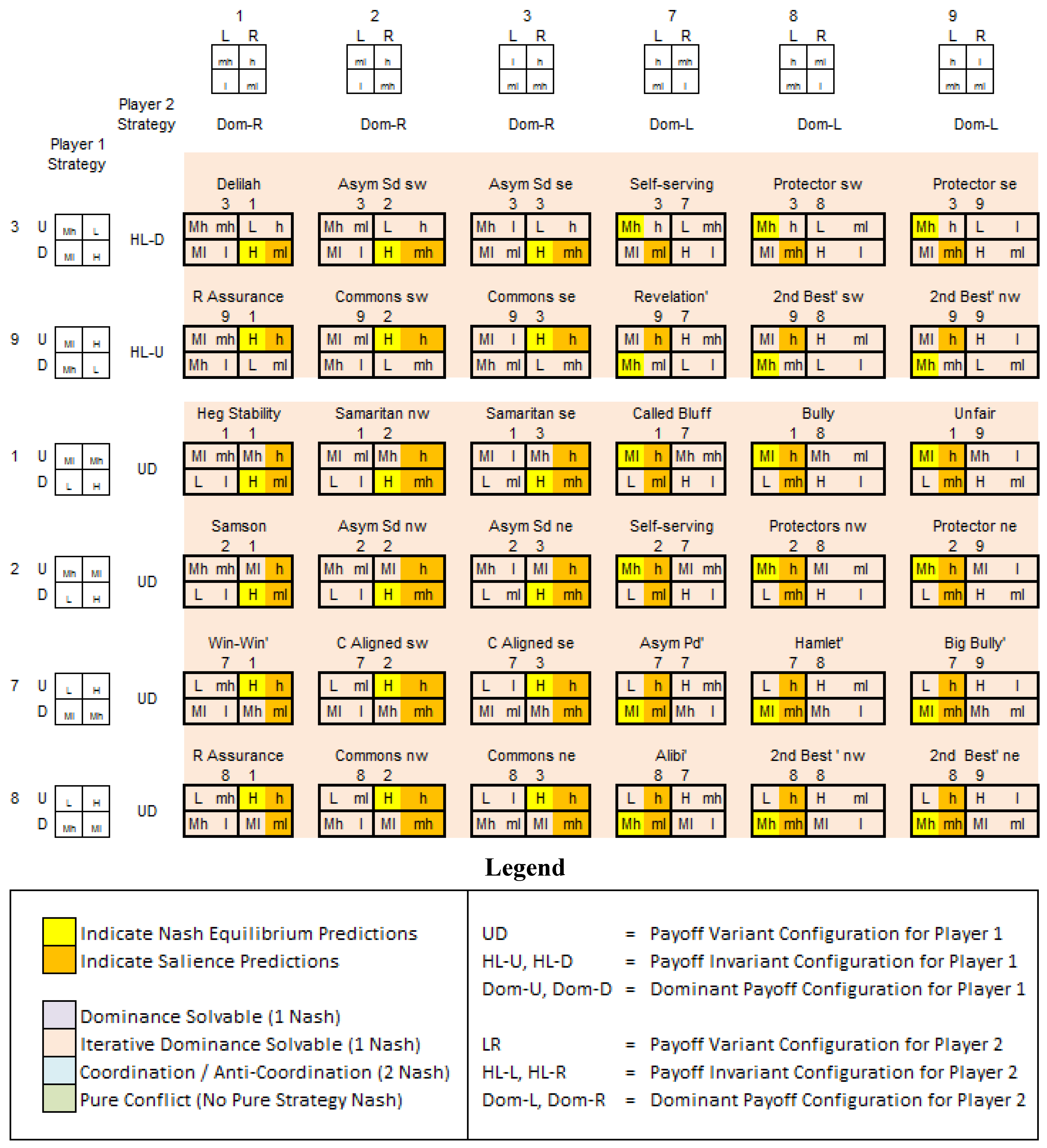
Figure 4.
The class of 144 strictly ordinal 2 × 2 games (games 7–1 through 12–6).
Figure 4.
The class of 144 strictly ordinal 2 × 2 games (games 7–1 through 12–6).
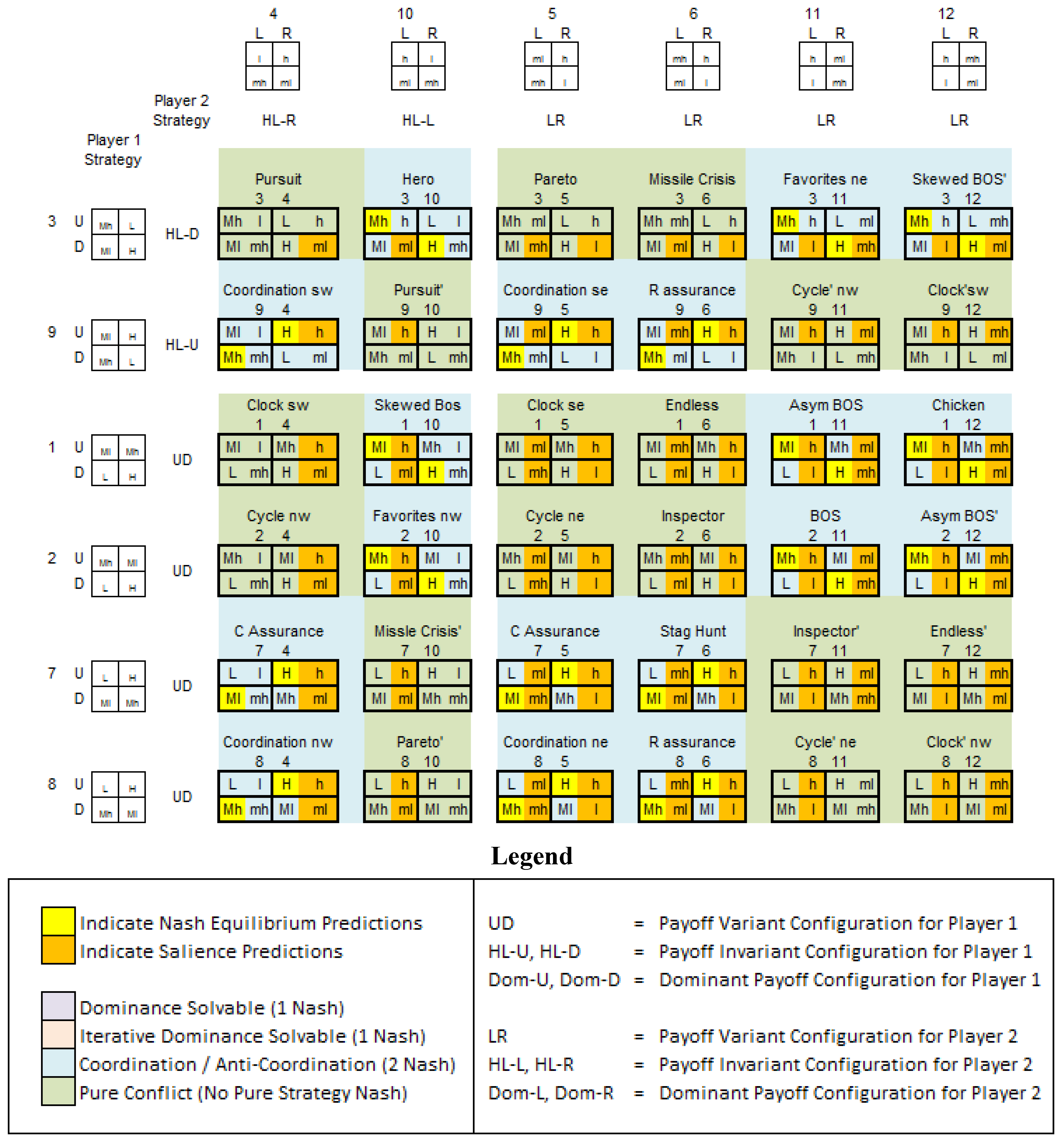
Figure 5.
The class of 144 strictly ordinal 2 × 2 games (games 7–7 through 12–12).
Figure 5.
The class of 144 strictly ordinal 2 × 2 games (games 7–7 through 12–12).
With the overall structure of the figures summarized, we now turn to finer details of the topology. In the tables, payoffs for Pl are ordered H, M
(edium)h
(igh), M
(edium)l
(ow), L
(ow) and are ordered h, mh, ml, l for P2. In each of
Figure 2,
Figure 3,
Figure 4 and
Figure 5, payoff structures for Player 1 are shown in the un-shaded matrices in the leftmost column. Payoff structures for Player 2 are shown in the un-shaded matrices in the top row. Notice that in all four tables there are sets of games solved by dominance (in purple) and by iterated dominance (in beige.)
Figure 5, like
Figure 2, contains a subset not solvable by game theory (in green). In contrast,
Figure 3 and
Figure 4 each contain a subset of games in blue. Those in
Figure 3 are anti-coordination games while those in
Figure 4 are coordination games.
Games that have been the focus of most inquiry in economics are those along the diagonal running from the lower-left to upper right in Figues 3 and 4. These include games involving varying degrees of preference incompatibility like the Prisoner’s Dilemma in the lower left and the Chicken game in the upper right (for
Figure 3) and games involving varying degrees of preference compatibility (from the “no conflict” game at one extreme to the stag-hunt at the other in
Figure 4).
Now consider the implications of strategy for behavior in these games. For a local player facing a payoff configuration with a dominating strategy (configurations labeled Dom-U(p) or Dom-D(own) and Dom-L(eft) or Dom-R(ight) in the figures), both differences in payoffs have the same sign. The dominant strategy will be selected either because one of the differences is larger, the payoffs associated with that difference are salient, and the player selects the strategy with the largest salient payoff, or because the differences are equal and the player checks for a dominant strategy.
For two other payoff configurations facing either player, the largest and smallest payoffs are juxtaposed. For these configurations, labeled H(igh)L(ow), the strategy corresponding to the larger payoff will be selected and this will be true independent of the values of the other payoffs. Payoff configurations for which this is the case are denoted HL-U(p) and HL-D(own) in the column labeled “Player 1 Strategy” and HL-L(eft) and HL-R(ight) in the row labeled Player 2 Strategy.
The third possible configuration of payoffs involves comparisons of the best and worst outcomes with outcomes of intermediate values where the differences are of opposing signs and different or equal magnitudes. These are the H(igh)I(ntermediate)/I(ntermediate)L(ow) payoff configurations and are simply labeled UD configurations (for Player 1) or LR configurations (for Player 2) in the figures since either strategy may be played depending on the precise payoff differences. For HI/IL payoff configurations where the differences are not equal, local players will choose the strategy associated with the larger salient payoff. Note however, that the identity of this strategy will vary with the values of the intermediate payoffs to the extent that changes in these values may reverse the absolute magnitudes of the differences. For HI/IL configurations where the differences are of equal magnitude and opposite sign, a local player will move on to consider the salience of his opponent’s payoffs. In
Figure 2,
Figure 3,
Figure 4 and
Figure 5, the strategy choices and game outcomes with local players when their own payoffs are salient are denoted in orange.
To provide a clearer picture of how the play of local players compares to that of fully rational ones,
Figure 6,
Figure 7,
Figure 8 and
Figure 9 reorder the payoff configurations from
Figure 2,
Figure 3,
Figure 4 and
Figure 5, presenting those payoff structures where there is a dominating strategy first, then the HL configurations, and then the HI/IL configurations. As before, the combined
Figure A2 is provided in the appendix.
As is clear in
Figure 6, because local players obey dominance, the predictions following from the model of salience-based play and from the Nash solution concept coincide in games where both players have dominating strategies. For cases depicted in
Figure 7 and
Figure 8 where one player has a dominant strategy but the other faces a HL or a HI/IL payoff structure, the former chooses the dominant strategy. The player facing a HL structure will choose the strategy offering the best possible outcome. As a consequence, in half of the Dom-HL cases, the outcomes following from iterated dominance and salience coincide (indicated by cells in games that are half yellow and half orange) whereas in the other half they diverge (where one cell in a game is yellow and another is orange). For a player facing a HI/IL configuration, the choice will vary as the relative magnitudes of the payoffs change the differences in payoffs across strategy choices. In Dom-HI/IL cases, the outcome predicted by salience coincides with that predicted by iterated dominance half the time but deviates the other half of the time.
Figure 6.
Strictly ordinal 2 × 2 games containing a dominant strategy equilibrium.
Figure 6.
Strictly ordinal 2 × 2 games containing a dominant strategy equilibrium.
Figure 7.
Strictly ordinal 2 × 2 dominance solvable games with dominant strategy for P1.
Figure 7.
Strictly ordinal 2 × 2 dominance solvable games with dominant strategy for P1.
Figure 8.
Strictly ordinal 2 × 2 dominance solvable games with dominant strategy for P2.
Figure 8.
Strictly ordinal 2 × 2 dominance solvable games with dominant strategy for P2.
Figure 9.
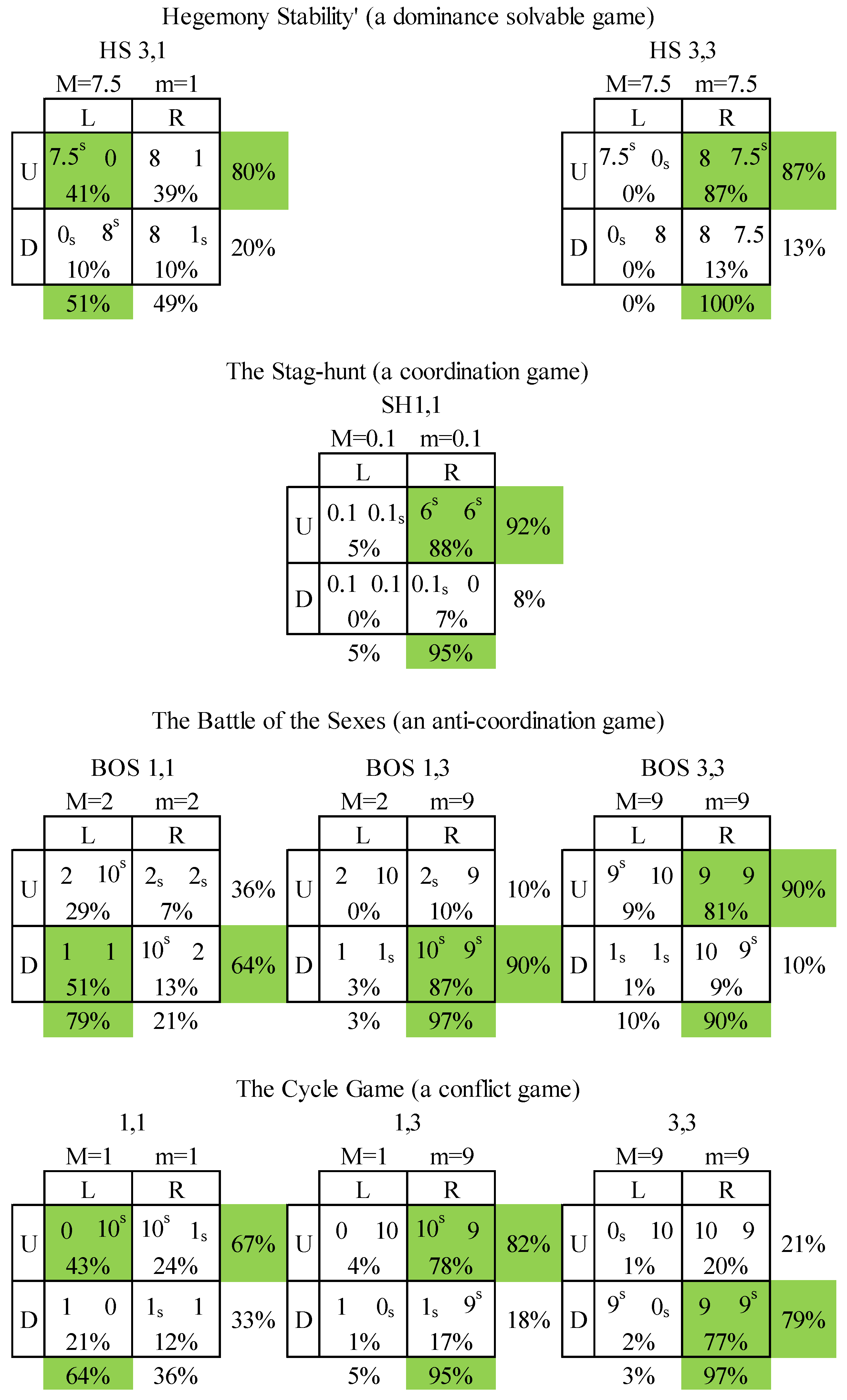
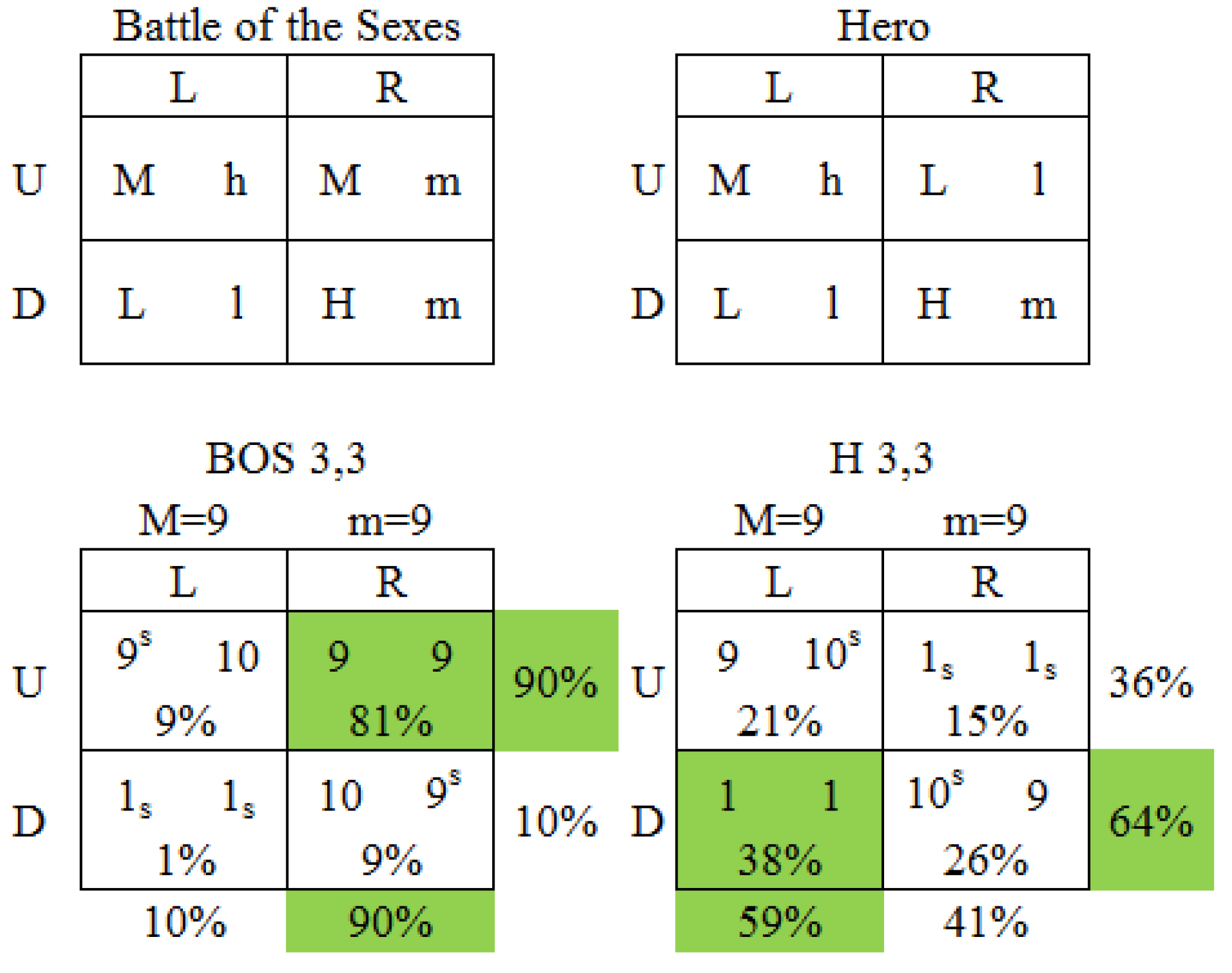
Strictly ordinal 2 × 2 games with zero or two pure-strategy Nash equilibria.
Figure 9.
Strictly ordinal 2 × 2 games with zero or two pure-strategy Nash equilibria.
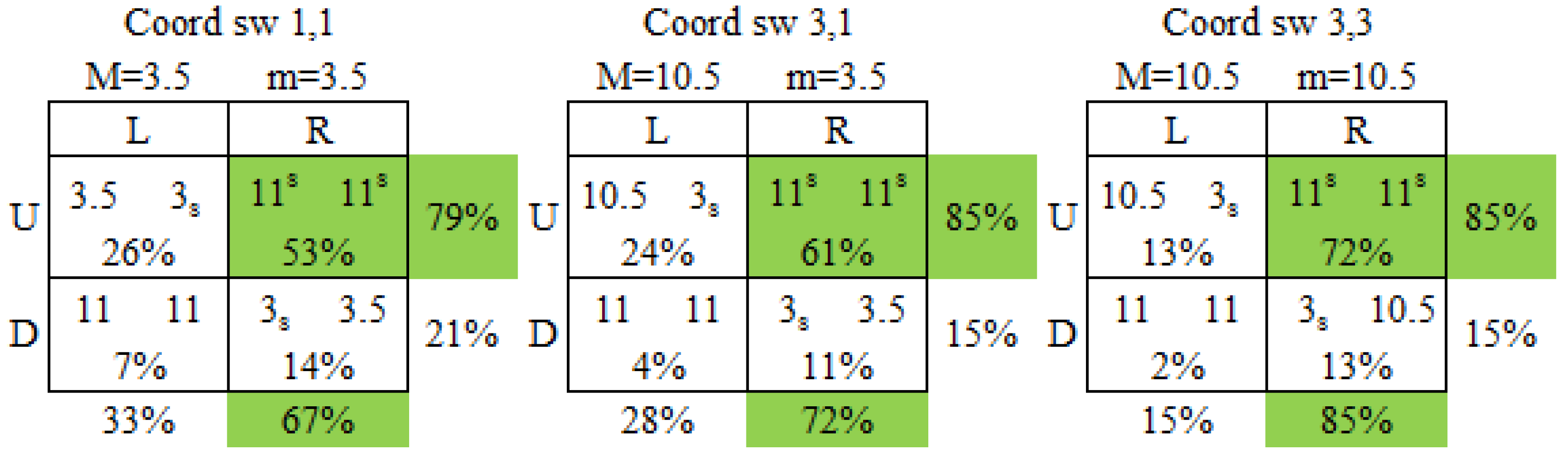
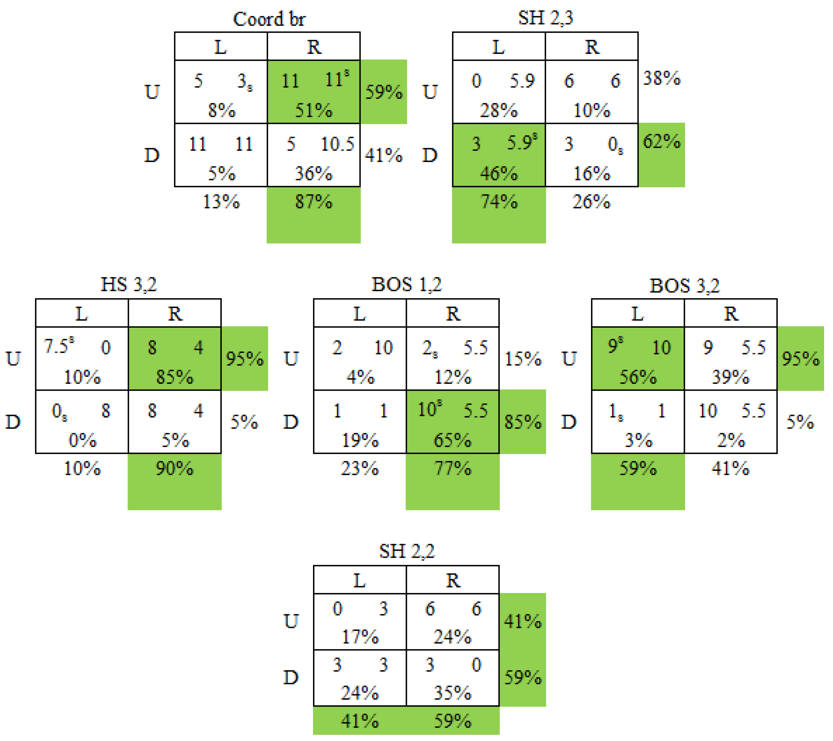
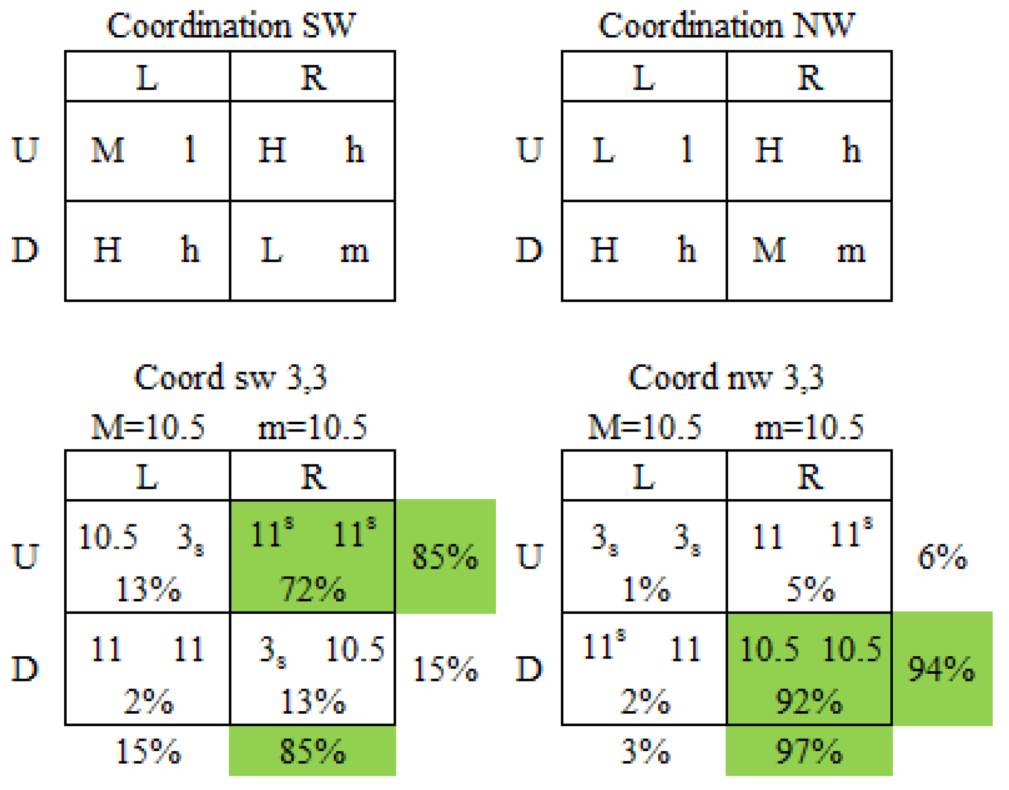
Figure 9 contains the games for which players face either HL or HI/IL payoff configurations. There are four games (those in the upper left corner of the matrix) where both players face HL payoff configurations. In these games, the model predicts that play will be invariant to the relative magnitudes of the payoffs (as is predicted for all games in traditional game theory). The predicted outcome in the Coordination sw game on the lower left corresponds to the payoff dominant Nash equilibrium. In the anti-coordination Hero game to the upper right (a variant of the Battle of the Sexes game), the predicted outcome is neither of the Nash equilibria. The other two HL/HL games are cyclic games in which there are no pure strategy Nash equilibria. In the remaining games in
Figure 9 (all involving either coordination, anti-coordination or cycles), own-payoff salience predicts either two or four outcomes as a function of the relative values of the intermediate payoffs for one or both players.
6 To summarize, in 2 × 2 games where the choice can be resolved by evaluation of a players’ own payoffs, there will be dominance solvable, coordination, anti-coordination and cyclic games involving Dom-HL or HL-HL payoff configurations for which the strategy choices and game outcomes will be invariant to the relative values of the payoffs. Henceforth, these are referred to as payoff-invariant games.
In contrast to the predictions of traditional game theory, there will also be dominance solvable, coordination, anti-coordination and cyclic games where strategy choices and the outcome of the game will be sensitive to the relative values of payoffs. In Dom-HI/IL games and HL-HI/IL games, 2 outcomes are possible. For HI/IL-HI/IL games, four outcomes are possible. We call these payoff-variant games. More generally, we state:
Definition 3: For a fixed ordinal ranking of payoffs, a game is payoff invariant if the outcome that occurs does not depend on the magnitudes of payoffs.
Proposition 2: A strictly ordinal 2 × 2 game played by local players is payoff invariant, if and only if it has the form of either Dom-Dom, Dom-HL, or HL-HL.
Proof: As illustrated in
Figure 2,
Figure 3,
Figure 4 and
Figure 5, there are six classes of payoff structures, depending on the configurations of the high, low, and intermediate payoffs for each player. These structures are Dom-Dom, Dom-HL, Dom-HI/IL, HL-HL, HL-HI/IL, and HI/IL-HI/IL. All 144 games in the figures can be classified into one of these structures. A configuration where both local players have dominant strategies (Dom-Dom) is payoff invariant (and will result in a Nash equilibrium) since the players always play their dominant strategies (each player either chooses the strategy with the largest salient payoff, which will be the dominant strategy if one exists, or chooses the dominant strategy when no payoffs are salient). When one player has a dominant strategy and the other player does not, but has his highest and lowest payoff in the same row (if he is a column player) or in the same column (if he is a row player) we have a Dom-HL configuration. This configuration is also payoff invariant (but will not necessarily induce a Nash equilibrium) since the local player with the dominant strategy continues to play that strategy, and the other local player always plays the strategy with his highest payoff (since the highest and lowest payoffs are salient, as the inequality
always holds for strict-ordinal games). Analogous reasoning leads us to conclude that HL-HL configurations are payoff invariant (but do not necessarily result in a Nash equilibrium). For an HI/IL configuration a local player either compares
and
or
and
. The particular direction of the inequality determines which payoffs are salient, and can thus influence the strategy choice since a local player plays the strategy with the larger salient payoff. Thus, games where either player has an HI/IL configuration are not payoff invariant. ∎
Note that the top row and the left-most column (not shaded) in
Figure 2,
Figure 3,
Figure 4,
Figure 5,
Figure 6,
Figure 7,
Figure 8 and
Figure 9 provide a more detailed characterization of the possible payoff structures for each player. Using these payoff structures, we can characterize the set of games played by local players (or by Level-1 boundedly rational players) for which a Nash equilibrium will
always obtain out of the entire set of 144 2 × 2 games.
As shown in
Figure 2,
Figure 3,
Figure 4,
Figure 5,
Figure 6,
Figure 7,
Figure 8 and
Figure 9, Player 1 has two possible strategies, U and D, and Player 2 has two possible strategies, L and R. We refer to particular strategies and payoff structures in the figures by a string of letters first noting the payoff structure and then the strategy determined by that structure for local players. For instance, HL-U corresponds to a HL payoff structure in which Player 1 plays U.
Proposition 3: A pure-strategy Nash equilibrium will always obtain in a 2 × 2 strictly ordinal game with local players if and only if the game has a dominant strategy equilibrium
or if it has one of the following payoff structures:
- (i)
HL-U/HL-R
- (ii)
HL-D/Dom-R
- (iii)
HL-U/Dom-R
- (iv)
Dom-U/HL-R
- (v)
Dom-U/HL-L
For general representations of these payoff structures, see the upper row and left-most column in
Figure 2,
Figure 3,
Figure 4,
Figure 5,
Figure 6,
Figure 7,
Figure 8 and
Figure 9. The observation that each of these payoff structures always yields a Nash equilibrium can be seen directly in
Figure 6,
Figure 7 and
Figure 8 since in these games, the orange cells (played by local players) always coincide with a yellow (Nash equilibrium) cell. The proof is straightforward and is thus omitted. There are a total of 49 games classified under Proposition 3 (36 games with dominant strategy equilibria, and 13 games classified in (i) through (v)). Thus, 49 out of 144 strictly ordinal 2 × 2 games will
always produce a Nash equilibrium for local players and players who are Level-1 boundedly rational, even though these players are not as strategically sophisticated as assumed in traditional game theory. There are additional games which may produce an equilibrium, depending on the payoff structure.
We can also characterize the set of 2 × 2 games played by local players (or by Level-1 players) for which a pure strategy Nash equilibrium will never obtain.
Proposition 4: A pure-strategy Nash equilibrium will never obtain in a 2 × 2 game with local players if and only if the game is a cyclic game
or if it has one of the following payoff structures:
- (i)
HL-D/HL-L
- (ii)
HL-D/Dom-L
- (iii)
HL-U/Dom-L
- (iv)
Dom-D/HL-R
- (v)
Dom-D/HL-L
The result that each of these payoff structures never yields an equilibrium can be seen directly in
Figure 7,
Figure 8 and
Figure 9 since in these games, the orange cells never coincide with a yellow (Nash equilibrium) cell. The proof is straightforward and is thus omitted. There are a total of 31 games classified under Proposition 4 (18 cyclic games, and 13 games classified in (i) through (v)). Thus, 31 out of 144 strictly ordinal 2 × 2 games will
never produce a Nash equilibrium for local players.
In total, Propositions 3 and 4 identify 80 payoff invariant games, indicating that in over half of all ordinal 2 × 2 games, the games are “rigged” for local players. They cannot escape the outcome of the strategic interaction they face. As noted in Proposition 1, these same predictions follow if subjects behave as Level-1 players in a Cognitive Hierarchy model. A Level-1 player chooses his strategy based on the assumption that the other player chooses between her strategies with equal probability—(i.e., choosing the strategy that maximizes expected utility given a uniform prior on the other player’s choices). For Dom payoff structures, the dominant strategy will always have a higher expected value than the dominated strategy. Similarly, for HL games, the expected value associated with the strategy containing H and Ml or H and Mh will always be greater than the expected value associated with the strategy containing Mh and L or Ml and L, respectively. For HI/IL structures, on the other hand, the expected value of the two strategies (e.g., H and L versus Mh and Ml) will vary with the values of the intermediate payoffs, but they do so in lockstep with differences H−Ml and Mh−L or H−Mh and Ml−L.
2.2. Implications of Other-Payoff Salience
We now consider the implications of the model when no payoffs are salient and neither strategy is dominant for Player 1. In this case, the cardinality of payoff differences must be the same for each pair of payoffs, obtained when holding Player 2’s strategy fixed:
These cases can only arise in situations where one or both players’ payoff configurations are of the HI/IL variety. When this occurs,
implies that an agent is spurred to think strategically and best responds to the strategy he anticipates his opponent will play given the perceived salience of the opponent’s payoffs.
Figure 10 and
Figure 11 summarize Player 1’s strategy choices conditional on the salience of Player 2’s payoffs for the relevant subset of the 144 games. The predicted outcomes of
are again in orange and the Nash equilibrium outcomes are in bold and yellow.
As is clear from
Figure 10 and
Figure 11, games that had two outcomes in
Figure 2,
Figure 3,
Figure 4,
Figure 5,
Figure 6,
Figure 7,
Figure 8 and
Figure 9 now have a single outcome and those that had four outcomes now have two. Note also that the outcome or outcomes predicted by
now coincide entirely with the Nash equilibrium outcome(s) when they exist. The reason is simple. The disequilibria outcomes in
Figure 2,
Figure 3,
Figure 4,
Figure 5,
Figure 6,
Figure 7,
Figure 8 and
Figure 9 only arise for two sets of cases. One set involves one player having a dominating strategy and the other’s salience perceptions recommending the non-equilibrium response. The second set involve coordination and anti-coordination games where one player’s salience perceptions lead him to choose the strategy consistent with one of the Nash equilibrium outcomes while the other player’s perceptions lead him to choose the strategy corresponding to the other equilibrium outcome.
7 When one player becomes strategic and best responds to the opponent’s salience-based strategy, the opponent’s play basically determines the outcome of the game. Note finally that
still makes unique predictions for games where there are no pure Nash equilibria.
Figure 10.
Implications of “other-payoff salience” in Dominance Solvable Games for Player 1.
8
Figure 10.
Implications of “other-payoff salience” in Dominance Solvable Games for Player 1.
8
Figure 11.
Implications of “other-payoff salience” in Cycle and Coordination Games for Player 1.
Figure 11.
Implications of “other-payoff salience” in Cycle and Coordination Games for Player 1.
Recall that in Proposition 1, we showed the observational equivalence of salience and Level-1 strategies for cases where each local player has salient payoffs. In this section, we considered the case where one local player has no salient payoffs. For games with a unique pure strategy Nash equilibrium, denote the Nash equilibrium strategy for P1 by (P1).
Proposition 5: Consider any 2 × 2 strictly ordinal game with a unique pure-strategy Nash equilibrium. If Player 1 has no salient payoffs or dominant strategies, and Player 2 does have salient payoffs, then strategies
(P1) and
(P1) are observationally equivalent.
9 Proof: In the absence of salient payoffs or dominant strategies for P1, strategy dictates that P1 best-responds to the salient or dominant strategy of P2. Note that since P2 has salient payoffs, the differences in payoffs between P2’s strategies are not equal and any dominant strategy for P2 will correspond to the strategy with the larger salient payoff. If P2 has a dominant strategy, then P1’s best-response to P2’s strategy clearly results in an equilibrium. If P2 does not have a dominant strategy, but has either an HL or HI/IL configuration, P2 will choose the strategy with the larger salient payoff. This strategy is always a best-response to an equilibrium strategy played by P1 (when a pure strategy equilibrium exists), and thus it is an equilibrium strategy for P2. Since P1 is playing his best-response to this equilibrium strategy for P2, the result will be the pure strategy Nash equilibrium ∎
Proposition 5 extends straightforwardly to 2 × 2 strictly ordinal games with multiple pure-strategy Nash equilibria, in which case strategy (P1) is observationally equivalent to one of the Nash equilibrium strategies.
Propositions 1 and 5 collectively predict instances when a local player will appear to be Level-1 boundedly rational, and when the same player will appear to be the rational economic agent assumed in game theory.
Note that the behavior predicted in Proposition 5 does not follow if players are Level-1. Level-1s base their strategy choices on the assumption that their opponent will choose randomly irrespective of the payoff values that the opponent faces.
For cases where both players’ own payoff comparisons are uninformative, local and Level-1 players choose at random.


