Estimating Case-Based Learning

Abstract

We propose a framework in order to econometrically estimate case-based learning and apply it to empirical data from twelve 2 × 2 mixed strategy equilibria experiments. Case-based learning allows agents to explicitly incorporate information available to the experimental subjects in a simple, compact, and arguably natural way. We compare the estimates of case-based learning to other learning models (reinforcement learning and self-tuned experience weighted attraction learning) while using in-sample and out-of-sample measures. We find evidence that case-based learning explains these data better than the other models based on both in-sample and out-of-sample measures. Additionally, the case-based specification estimates how factors determine the salience of past experiences for the agents. We find that, in constant sum games, opposing players’ behavior is more important than recency and, in non-constant sum games, the reverse is true.

1. Introduction

Economists across the discipline—micro and macro, theory and empirics—study the impact of learning on individual and social behavior. Two questions are typical of this inquiry: first, whether and when learning leads to equilibrium behavior, and second, which model(s) of learning best explain the data. In this paper, we formulate a method to econometrically estimate Case-based Decision Theory (CBDT), introduced by Gilboa and Schmeidler [1], on individual choice data.

Like Expected Utility (EU), CBDT is a decision theory: that is, it shows that if an agent’s choice behavior follows certain axioms, it can be rationalized with a particular mathematical representation of utility e.g., Von Neumann and Morgenstern [2], Savage [3]. The Expected Utility framework has states of the world, actions, and payoffs/outcomes. The CBDT framework retains actions and payoffs, but it replaces the set of states with a set of “problems”, or circumstances; essentially, vectors of information that describe the choice setting the agent faces. CBDT postulates that when an agent is confronted with a new problem, she asks herself: how similar is today’s problem to problems in memory? She then uses those similarity-weighted problems to construct a forecasted payoff for each action, and chooses an action with the highest forecasted payoff.

The primary motivation for our study is to estimate and measure the efficacy of CBDT to explain learning. Therefore, in this context, we refer to Case-based Learning or CBL. We develop a framework to estimate dynamic case-based decision theory econometrically and test it in a game-theoretic setting against other learning models. One significant difference between CBL and other learning models is the formulation of how information enters into decision-making. In CBL, information enters in how agents perceive past experiences to be salient to current choice. To do this, CBL incorporates psychological similarity.

An important part of this work is using a stochastic choice rule to estimate CBDT. CBDT is a deterministic theory of choice, but, in this study, we transform it into stochastic choice. The primary purpose of this transformation is estimating parameters of models on data, like much of the literature in learning algorithms that we compare CBDT against. However, it is worth noting that there is precedent in the literature to treat CBDT specifically as stochastic, e.g., Pape and Kurtz [4] and Guilfoos and Pape [5] use stochastic forgetfulness in their implementations to match human data. Moreover, there is a broader tradition in psychology of converting deterministic utility valuations into stochastic choice through the so-called Luce choice rule or Luce choice axiom [6] (see Section 3.6).

We test CBL and other learning models on data from a series of 2 × 2 experimental mixed strategy equilibria games. Erev and Roth [7] make an explicit case for the use of unique mixed strategy equilibrium games to investigate learning models, in part because the number of equilibria does not change with finite repetitions of the game and the equilibrium can be achieved in the stage game. Given the simplicity of the information available to subjects, these data provide a relatively conservative environment for a researcher to test CBL, as it restricts the degrees of freedom to the researcher. In an experiment, the information available to subjects is tightly controlled, so a well-defined experiment provides a natural definition of the problem vector for CBDT. We estimate parameters of the learning algorithms to understand how parameters change under different contexts, and because they provide information about the nature of choice. A benefit of estimating parameters of CBL is to compare how stable the parameters remain under different contexts. The data we use are well-studied by researchers investigating stationarity concepts and learning models [8,9].

We find that CBL explains these empirical data well. We show that CBL outperforms other learning algorithms on aggregate on in-sample and out-of-sample measures. Reinforcement learning and CBL perform similarly across individual games and they have similar predictions across games. This is also supported by our analysis of the overlap in RL and CBL in attraction dynamics when certain restrictions are made. When learning models outperform the known equilibria or stationary concepts (Nash Equilibrium, action-sampling equilibrium, payoff-sampling equilibrium, and impulse balance equilibrium) it prompts the question of which learning models characterize the data well and what insights are gained through learning models into decision making behavior.1 For instance, it is known that some of the learning models in games do not converge to Nash Equilibrium and then we must consider what is it converging to, if anything, and how is it converging.

Our econometric framework for CBL provides estimates that measure the relative importance for each piece of information available to subjects and the joint significance of information in predicting individual choice; this can be interpreted as estimates of the salience of past experiences for the agents. We find that both recency and opposing players’ behavior are jointly important in determining salience. We also find that in constant sum games, the behavior of opposing players is more important than recency, while, in non-constant sum games, recency is more important. The relative importance (as revealed by the relative weights) provides new insight into how subjects respond to stimuli in mixed strategy games, and provides a new piece of empirical data for future theory models to explain and understand. This points toward future work, in which more studies interact learning models with available information to identify how learning occurs in and across games.

We compare CBL to two learning models from the literature: Reinforcement Learning [7]; and self-tuning Experience Weighted Attraction [10]. Reinforcement Learning (RL) directly posits that individuals will exhibit behavior that in the past has garnered relatively high payoffs. Self-tuning Experience Weighted Attraction (self-tuning EWA) is a model that allows for the learners to incorporate aspects of reinforcement learning and belief learning. Both have achieved empirical success in explaining experimental game play; in particular, these two were the most successful learning models tested in Chmura et al. [9], whose data we analyze. We describe these models in greater detail in Section 3. We also formally investigate the relationship between CBL and RL; we show there is a mapping between RL and CBL when particular assumptions are imposed on both. Relaxing these assumptions is informative in understanding how the algorithms relate.

There is a small but persuasive literature evaluating the empirical success of CBDT. It has been used to explain human choice behavior in a variety of settings in and outside the lab. There are three classes of empirical studies. The first class uses a similarity function as a static model, which ignores dynamics and learning [11,12]. The second class is dynamic, but it utilizes simulations to show that case-based models match population dynamics rather than econometric techniques to find parameters [4,5]. The third class is experimental investigations of different aspects of case-based decision-making [13,14,15,16,17,18]. Our study is unique in that it proposes a stochastic choice framework to estimate a dynamic case-based decision process on game theoretic observations from the lab. Further, we relate this estimator to the learning and behavioral game theory literature and demonstrate the way in which case-based learning is different.

Neuroeconomic mechanisms also suggest that CBDT is consistent with how past cases are encoded and used in order to make connections between cases when a decision-makers faces a new situation [19]. Neuroeconomics is also in agreement with many other learning models. It is hypothesized by Gayer and Gilboa [20] that, in simple games, case-based reasoning is more likely to be discarded in favor of rule-based reasoning, but case-based reasoning is likely to remain in complex games. CBDT is related to the learning model of Bordalo et al. [21], which uses a similarity measure to determine which past experiences are recalled from memory. This is related to CBDT: in Bordalo et al. [21], experience recall is driven by similarity, while, in CBDT, how significant an experience weighs in utility is driven by similarity. Argenziano and Gilboa [22] develop a similarity-based Nash Equilibria, in which the selection of actions is based on actions that would have performed best had it been used in the past. While the similarity-based equilibria are closely related to this work, our case-based learning is not an equilibrium concept. Our work builds on the empirical design developed in the applied papers as well as those developing empirical and functional tools related to CBL e.g., [23,24].

2. Applying Case-Based Learning to Experiments

First, we compare the case-based approach to traditional expected utility. The expected utility framework requires that the set of possible states is known to the decision-maker and that the decision-maker has a belief distribution over this set of states. Case-based decision theory replaces the state space and its corresponding belief distribution with a “problem” space—a space of possible circumstances that the decision-maker might encounter—and a similarity function defined over pairs of problems (circumstances). One limitation of the expected utility approach is that it is not well-defined for the decision-maker to encounter a truly “new” state, which is, a state the decision-maker had never thought of before (it could be modeled as a state that occurs with probability zero, but then Bayesian updating would leave it at probability zero). The case-based approach overcomes this difficulty: the decision-maker can naturally encounter a “new” problem or circumstance, and need only be able to judge how similar that problem is to other problems the decision-maker has encountered: no ex-ante determination is required.2 The problem space is also, arguably, more intuitive for many practical decision-making problems than the corresponding state space. For example, consider the problem of hiring a new assistant professor, where one’s payoff includes the success of this candidate, fit with the current department, willingness of the candidate to stay, etc. Describing each candidate as a vector of characteristics that can be judged more or less similar is fairly intuitive, while constructing a corresponding state space—possible maps of candidates to payoff-relevant variables—may not be. Reasoning by analogy, through similarity, can also make complex decisions more manageable. Moreover, the similarity between vectors of characteristics provides a specific means of extrapolating learning about one candidate to other candidates; the assumption of prior distributions, and updating those distributions, provides less guidance about how that extrapolation should be done.

In our setting multiple games are played in a laboratory in which players interact with each other to determine outcomes. The state space in this setting is large. The broadest interpretation of the appropriate state space is: the set of all possible maps from all possible histories of play with all opponents to all future play. While this is quite general, learning (that is, extrapolation from past events to future ones) requires the specification of a well-informed prior; if literally any path of play is possible given history, and if one had a diffuse (i.e., “uninformed”) prior over that set, then any future path is equally likely after every possible path of play. Alternatively, the state space might assume a limited set of possible player types or strategies; in that case, the state space would be all possible mappings of player types/strategies to players. While this provides more structure to learning, it requires that the (correct) set of possible player types is known.

On the other hand, defining an information vector about history is less open-ended. There are natural things to include in such a vector: the identity (if known) of the player encountered; the past play of opponents, a time when each action/play occurred; and, perhaps other features, such as social distance [26] or even personality traits [27]. This implies a kind of learning/extrapolation in which the behavior of player A is considered to be more relevant to predictions of A’s future behavior than is the behavior of some other player B; that if two players behave in a similar way in the past; that learning about one player is useful for predicting the play of another; and, that more recent events are more important than ones far in the past. These implications for learning naturally arise from a similarity function that considers vectors closer in Euclidean distance to be more similar (as we do here).3 Interestingly, others have adopted the concept of similarity as a basis of choice in cognitive choice models [28].4

Note that this kind of extrapolation can be constructed in a setting with priors over a state space, under particular joint assumptions over the prior over the state space and the state space itself. Case-based decision theory can be thought of as a particular set of testable joint assumptions that may or may not be true for predicting human behavior.

3. Learning Algorithms

Learning models in economics have served dual purposes. First, learning algorithms can play a theoretical role as a model of dynamics which converge to equilibrium. This is the explicit goal of the “belief learning” model [29]. Second, learning algorithms can play an empirical role in explaining the observed dynamics of game play over time. This goal is explicit in the “reinforcement learning” model [7] which draws heavily on models from artificial intelligence and psychology.

Both purposes are incorporated in the Experience Weighted Attraction model, which, appropriately enough, explicitly incorporates the belief learning and reinforcement learning models [30,31,32]. EWA and its one parameter successor, self-tuning EWA, has proved to be a particularly successful account of human experimental game play. Here, we discuss these reinforcement and self-tuning EWA models and compare and contrast them to the case-based learning approach.

In the following repeated games, we assume the same following notation: there are a set of agents indexed by $i=1,\dots ,n$, each with a strategy set $S_i$, which consists of $m_i$ discrete choices, so that $S_i=\left\{s_i^1,\dots ,s_i^{m_i}\right\}$. Strategies are indexed with j (e.g., $s_i^j$). Let $s=\left(s_1,s_2,\dots ,s_n\right)$ be a strategy profile, one for each agent; in typical notation, $s_{-i}$ denotes the strategy profile with agent i excluded, so $s_{-i}=\left(s_1,\dots ,s_{i-1},s_{i+1},\dots ,s_n\right)$. Scalar payoffs for player i are denoted with the function ${\pi }_i(s_i,s_{-i})$. Finally, let $s_i\left(t\right)$ denote agent i’s strategy choice at time t, so $s_{-i}\left(t\right)$ is the strategy choices of all other agents at time t.

Erev and Roth [7] argue that, empirically, behavior in experimental game theory appears to be probabilistic, not deterministic. Instead of recommending deterministic choices, these models offer what the EWA approach has come to call “attractions”. An attraction of an agent i to strategy j at time t is a scalar which corresponds to the likelihood that agent will choose this strategy at this time relative to other strategies available to this agent. An attraction by agent i to strategy j at time t under an arbitrary learning model will be represented by $A_i^j\left(t\right)$. We compare these models by saying that different models provide different functions which generate these attractions, so we will have, e.g., $CB{A}_i^j\left(t\right)$ to represent the attraction that is generated by the case-based model.

Because a given attraction corresponds to a likelihood, a vector of attractions ${\left\{A_i^j\left(t\right)\right\}}_{j=1}^{m_i}$ corresponds to a probability distribution over available choices at time t and, therefore, fully describes how this agent will choose at time t.5

We consider case-based learning (CBL), reinforcement learning (RL), and self-tuning experience weighted attraction (EWA), in turn.

3.1. Case-Based Learning

We bring a formulation of case-based decision theory as introduced by Gilboa and Schmeidler [1] into the “attraction” notation discussed above, ultimately ending up with a case-based attraction $CB{A}_i^j\left(t\right)$ for each strategy $s_j$.

The primitives of Case-Based Decision Theory are: a finite set of actions $\mathcal{A}$ with typical element a, a finite set of problems $\mathcal{P}$ with typical element p, and a set of results $\mathcal{R}$ with typical element r. The set of acts is of course the same as the set of actions or strategies as one would find in a typical game theoretic set-up. The set of problems can be thought of a set of circumstances that the agent might face: or, more precisely, a vector of relevant information about the present circumstances surrounding the choice that the agent faces, such as current weather, time of day, or presence of others. The results are simply the prizes or outcomes that result from the choice.

A problem/action/result triplet $\left(p,a,r\right)$ is called a case and can be thought of as a complete learning experience. The set of cases is $\mathcal{C}$ $=\mathcal{P}\times \mathcal{A}\times \mathcal{R}$. Each agent is endowed with a set $\mathcal{M}$ ⊆ $\mathcal{C}$, which is called the memory of that agent. Typically, the memory represents those cases that the agent has directly experienced (which is how it is used here) but the memory could be populated with cases from another source, such another agent or a public information source.

Each agent is also endowed with a similarity function $s:\mathcal{P}\times \mathcal{P}\to {\mathbb{R}}_{+}$, which represents how similar two problems are in the mind of the agent. The agent also has a utility function $u:\mathcal{R}\to \mathbb{R}$ and a reference level of utility $H$, which is called the aspiration value. An aspiration value is a kind of reference point. It is the desired level of utility for the agent; when the agent achieves her aspiration value of utility, she is satisfied with that choice and is not moved to seek alternatives.

When an agent is presented with problem p, the agent constructs the case-based utility for each available action $a\in \mathcal{A}$ and selects an action with the highest CBU.6 CBU is constructed from memory in Equation (1).

$$CBU(p,a)=\sum _{\left(q,a,r\right)\in \mathcal{M}\left(a\right)}s(p,q)\left[u\left(r\right)-H\right]$$

(1)

where $\mathcal{M}\left(a\right)$ is defined as the subset of memory in which act a was chosen; that is $\mathcal{M}\left(a\right)=\left\{(q,a,r)\left|\right(q,a,r)\in \mathcal{M}\right\}$. (Following Gilboa and Schmeidler [1], if $\mathcal{M}\left(a\right)$ is the empty set—that is, if act a does not appear anywhere in memory—then $CBU(p,a)$ is assumed to equal zero.)

The interpretation of case-based utility is that, to form a forecast of the value of choosing act a, the agent recalls all those cases in which she chose action a. That typical corresponding case is called $(q,a,r)$. The value associated with that case is the similarity $s(p,q)$ between that case’s problem q and her current problem p, times the utility value of the result of that decision, minus the aspiration value $H$. Subsequently, her total forecast is the sum of those values across the entire available memory.

Now, let us bring the theory of case-based learning to an empirical strategy for estimating case-based learning in these experiments. Note that the experiments studied here—2 × 2 games with information about one’s history—provide an environment for testing the theory of case-based learning, because the information vectors $\mathcal{P}$ presented to subjects is well-understood and controlled by the experimenter. (Outside the lab, more and stronger assumptions may be required to define $\mathcal{P}$).

3.1.1. Definition of Case-Based Attraction

CBL is defined by Equation (2). $CB{A}_i^j\left(t\right)$ is the case-based attraction of agent i to strategy j at time t; as discussed above, an attraction corresponds to the probability of selecting a strategy j. Here we present the equation and discuss each component in turn:

$${\displaystyle CB{A}_i^j\left(t\right)=A_0^j+\sum _{m=\max (t-M,0)}^{t-1}I(s_i^j,s_i\left(m\right))·S(x_t,x_m)·[\pi \left(s_i\left(m\right)\right)-H]}$$

(2)

The first term, $A_0^j$, is a taste parameter for strategy j. On the first instance of play, the second term is zero (we will explain below), so $A_0^j$ also equals the initial attraction to strategy j. On the first instance of play, there are no prior cases to inform the experimenter of the subject’s preferences, so it might be natural to assume that the agent ought to be indifferent among all actions, which would suggest that agents ought to choose all actions with equal probability in the first round. This does not appear to be the case in the data, hence the inclusion of this taste parameter (if initial actions are selected with equal probabilities, then these taste parameters will be estimated to be equal).

Now, let us consider the second term:

$${\displaystyle \sum _{m=\max (t-M,0)}^{t-1}I(s_i^j,s_i\left(m\right))·S(x_t,x_m)·[\pi \left(s_i\left(m\right)\right)-H]}$$

The variable M the (maximum) length of memory considered by the agent. The first case considered by the agent is listed as $m=\max (t-M,0)$. This has a straight-forward interpretation: either considered memory begins at period 0, which is the beginning, or, if $t>M$ (and, therefore, $t-M>0$), then only the last M periods are considered in memory. For example, if $M=3$, then every utility calculation only considers the last three periods. If all experiences are included in memory then M is equal to ∞. We test the importance of the choice of M in the Section 6.

$I(s_i^j,s_i\left(m\right))$ is an indicator function that maps cases in memory to the appropriate attraction for the strategy chosen: that is, when the strategy chosen, $s_i\left(m\right)$, is equal to strategy $s_i^j$, then this function equals one and it contributes to the attraction for strategy $s_i^j$. Otherwise, this function is zero and it does not contribute.

$S(x_t,x_m)$ is the similarity function, which translates the elements of the problem into relevance: the greater the similarity value, the more relevant problem $x_m$ is to problem $x_t$ to the decision-maker.

$[\pi \left(s_i\left(m\right)\right)-H]$ is the payoff in memory, net the aspiration level, so results that exceed aspirations are positive and results that fall short of aspirations are negative.

3.1.2. The Functional Form of Similarity

We give a specific functional form to the similarity function in Equations (3) and (4), where x and y denote two different problem vectors. We choose an inverse exponential function that uses weighted Euclidean distance between the elements of the circumstances to measure the similarity of situations. This choice has support from the psychology literature [33]. Specifically, the information that individuals encounter in past experiences and can observe in the current case are compared through the similarity function. The more similar the current case to the past case, the greater weight the past case is given in the formulation of utility. (We explore other functional forms of similarity and distance between information vectors in Section 7.2.).

$$\begin{array}{ccc}\hfill S(x,y)& =& \frac{1}{{\mathrm{e}}^{d(x,y)}}\hfill \end{array}$$

(3)

$$\begin{array}{ccc}\hfill \mathrm{where}d(x,y)& =& \sqrt{{\displaystyle \sum _{i=1}^{\#Dims}{w}_i\left[{(x_i-y_i)}^2\right]}}\hfill \\ \hfill & & \mathrm{for}\mathrm{some}\mathrm{weights}{w}_i.\hfill \end{array}$$

(4)

3.1.3. Comparision to RL And EWA

In RL and self-tuning EWA, attractions at time t are a function of attractions at time $t-1$, and attractions explicitly grow when the strategies they correspond to are valuable to the agent, a process called ‘accumulation’. Note that CBL does not explicitly accumulate attractions in this way, and has no built-in depreciation or accumulation factor such as $\varphi$ or $\frac{N\left(t\right)}{N(t-1)}$. However, closer inspection suggests that CBL implicitly accumulates attractions through how it handles cases in memory: as new cases enter memory, when payoffs exceed the aspiration level, they increase the attraction of the corresponding strategy. This appears to function as explicit accumulation does in the other theories. One important difference between the case-based approach to accumulation and the RL/EWA method is dynamic re-weighting: that is, when the current problem (information vector) changes, the entire memory is re-weighted by the corresponding similarity values. There is accumulation of a sort, but that accumulation is information-vector dependent. Accumulation through similarity allows for CBL to re-calibrate attractions to strategies that are based on information in the current and past problem sets.7

Depreciation can also be modeled in a natural way in CBL: if time is a characteristic in the information vector, then cases further in the past automatically play a diminishing role in current utility forecasts as they become more dissimilar to the present.

3.2. Reinforcement Learning

Reinforcement learning (RL) has origins in psychology and artificial intelligence and it is used in many fields, including neuroscience [34,35]. This is the formulation that we use here:

Consider a vector of attractions ${\left\{RL{A}_i^j\right\}}_{j=1}^{m_i}$. Suppose that strategy $s^j$ is chosen, the payoff experienced by agent i is added to $RL{A}_i^j$. In this way, strategies that turn out well (have a high payoff) have their attraction increased, so they are played more likely in the future. After strategy profile $s\left(t\right)$ is chosen at time t and payoffs are awarded, the new vector of attractions is:

$$RL{A}_i^j\left(t\right)=\varphi RL{A}_i^j(t-1)+I\left(s_i^j\left(t\right),s_i^j\right)·{\pi }_i\left(s_i,s_{-i}\left(t\right)\right)\forall j=1,\dots ,m_i$$

(5)

This is the same basic model of accumulated attractions as proposed by Harley [36] and Roth and Erev [37]. The first term within the brackets, $\varphi RL{A}_i^j(t-1)$, captures the waning influence of past attractions. For all attractions other than the one corresponding to the selected strategy $s\left(t\right)$ attractions tend toward zero, assuming that the single global factor is not too large. $I(s_i^j,s_i\left(t\right))$ will be used to denote the indicator function which equals 1 when $s_i^j=s_i\left(t\right)$ and 0 otherwise. The one countervailing force is the payoff ${\pi }_i$, which only plays a role in the selected strategy (as indicated by the indicator function). This version of reinforcement learning is a cumulative weighted RL, since payoffs accumulate in the attractions to chosen strategies. In a simplified setting where payoffs are weakly positive, this process can be thought of as a set of leaky buckets (with leak rate $\left(1-\varphi \right)$), one corresponding to each strategy, in which more water is poured into buckets corresponding to the strategy chosen in proportion to the size of the payoff received.8 Subsequently, a strategy is chosen with a probability that corresponds to the amount of water in its bucket.

There are simpler forms of RL that can be used, where $\varphi$ is equal to 1, and not estimated. This simpler model is estimated in Chmura et al. [9] and performs worse than our modified model in explaining the data. We use Equation (5) to fit the data to make conservative comparisons to the CBL model.

3.3. Self-Tuning Experience Weighted Attraction

Self-tuning experience weighted attraction was developed by Ho et al. [10] to encompass experience weighted attraction [31] in a simple one parameter model. EWA incorporates both RL and belief learning, which relies on so-called “fictitious play”, in which the payoffs of forgone strategies are weighted alongside realized payoffs. Self-tuning EWA is a compact and flexible way to incorporate different types of learning in one algorithm.

Equation (6) describes self-tuning EWA: a $\delta$ weight is placed on fictitious play and a $\left(1-\delta \right)$ weight is placed on realized outcomes. Self-tuning EWA has been successful at explaining game play in a number of different settings, including the data that we use in this paper.

$$EW{A}_i^j\left(t\right)=\frac{N(t-1)\varphi \left(t\right)EW{A}_i^j(t-1)+\left[\delta +(1-\delta )·I(s_i^j,s_i\left(t\right))\right]·\pi (s_i^j,s_{-i}\left(t\right))}{N\left(t\right)}$$

(6)

In self-tuning EWA, the parameter N evolves by the rule $N\left(t\right)=\varphi ·N(t-1)+1$ and $N\left(0\right)=1$. The $I(·)$ function is an indicator function that takes a value of 1 when $s\left(t\right)=s_i$ and 0 otherwise. The parameter $\varphi$ acts as a discount on past experiences, which represents either agents forgetfulness or incorporating a belief that conditions of the game may be changing. This parameter evolves, so that $\varphi \left(t\right)=1-\frac{1}{2}Sp\left(t\right)$, where $Sp\left(t\right)$ is a surprise index. $Sp\left(t\right)$ measures the extent to which agent’s partners deviate from previous play. More precisely, it is defined by the cumulative history of play $h_j^k\left(t\right)$ and a vector of the most recent play $r_j^k\left(t\right)$ for strategy j and opposing player k, as given in the Equations (7) and (8).

$$h_j^k\left(t\right)=\frac{{\sum }_{\tau =1}^{t}I(s_j^k,s^k\left(\tau \right))}{t}$$

(7)

$$r_j^k\left(t\right)={\displaystyle \sum _{j=1}^2}\frac{{\sum }_{\tau =t-W+1}^{t}I(s_j^k,s^k\left(\tau \right))}{W}$$

(8)

$W=2$ because there are only two strategies available to all agents in these games. In the experiments used in this paper, the subjects are unable to identify opposing players and we treat all of the opposing players as a representative average player, following Chmura et al. [9], to define histories and the surprise index. Equation (9) defines the surprise index, which is the quadratic distance between cumulative and immediate histories.

$$Sp\left(t\right)={\displaystyle \sum _{j=1}^2}{(r_j^k\left(t\right)-h_j^k\left(t\right))}^2$$

(9)

The fictitious play coefficient $\delta$ shifts attention to the high payoff strategy. This function takes the value of $\delta =\frac{1}{W}$ if $\pi (s_i,s_{-i}\left(t\right))>\pi \left(t\right)$ and 0 otherwise.

3.4. Relationship between RL and CBL

There is a strong connection between case-based learning and other learning algorithms, particularly reinforcement learning. One way to illustrate the connection between RL and CBL is by constraining both RL and CBL in particular ways, so that they become instances of each other. Subsequently, we can consider the implications of relaxing these constraints and allowing them to differ.

On CBL, we impose three restrictive assumptions: first, we constrain the information vector to include only time (so that the only aspect of situations/problems that the case-based learner uses to judge similarity is how close in time they occurred). Second, we set the aspiration level to zero, so that payoffs are reinforced equivalently in RL and CBL. Third, we assume the similarity function is of the form in Equation (10).

$$S(x_t,x_m)=\frac{1}{w^{|t-m|}}.$$

(10)

(Note, again, that $x_t$ is a ‘vector’, which consists only of t).

Finally, on both, we impose the assumption that initial attractions to be zero for both CBL and RL, which means that, in both cases, choices are randomized in the initial period.

We can then derive the weight in similarity that leads to the same decay in attractions in both RL and CBL, as displayed in Equation (11).

$$\varphi =S(x_t,x_{t-1})=\frac{1}{w}$$

(11)

Under the assumptions on RL and CBL listed above, if one estimates the RL equation (Equation (5)) and then estimates the CBL equation (Equation (2)) on the same data, and then resulting estimators $\varphi$ and w are necessarily related in the way described in Equation (11). We do not use these specialized forms to estimate against the data, but rather use them to demonstrate the simple similarities and differences in how CBL and RL are constructed. In Appendix A, we provide more details on the formal relationship between RL and CBL.

This is a base case, where RL and CBL are the same. Now, let us consider two complications relative to this base case and consider the implications for the different attractions.

First, let us allow for more variables in the information vector (in addition to time) and consider how this would change the CBL agent relative to the RL/base case agent. Adding more variables to the information vector can be thought of as a CBL agent being able to maintain multiple ‘rates of decay’, which could vary over time, where the CBL agent can choose which ‘rate of decay’ to use based on the current situation. For example, suppose opponent ID is included in the information vector. Subsequently, if the agent is playing a partner they encountered two periods ago, the CBL agent could choose to downweight the previous period’s attraction and increase the weight given to the problem from two periods ago. In essence, this additional information, and combination of weights in the definition of distance, allows for the $\varphi$ parameter to be ‘recast’ based on the memory of an agent and the current problem. The modification of reinforcement learning to include the recasting is an elegant way to incorporate the multiple dimensions of information agents use when playing games. It suggests that other empirical applications in discrete choice may also benefit in using CBL, because it contains core elements of reinforcement learning that have been successful in modeling behavior.

Second, let us consider an aspiration level that differs from zero. Suppose payoffs $\pi \ge 0$, as they are in the games that we consider here. Subsequently, under RL, and under CBL with $H=0$, every experience acts as an attractor: that is, it adds probability weight to a particular action, the question is: how much probability weight does it add. However, when $H>0$, then the change in attraction of an action is does not increase in $\pi$, but rather in $\pi -H$. This, importantly, changes the implications for attraction for payoffs that fall short of H. Under CBDT, such payoffs provide a “detractor” to that action, so they directly lower the attraction corresponding to this action.

3.5. Initial Attractions

We estimate initial attractions to strategies for all learning models. This adds two additional parameters to estimate for all models, for the row player the initial attraction to strategy Up and for the column player the initial attraction to strategy Left. This seems sensible, because, empirically, it does not appear that subjects choose strategies randomly in the first period of play, and, a priori, there is a systematic difference between payoffs when considering the expected play by the opposing player. We can compare the actions in the first round of the experimental data to the estimated initial attractions as a sensible test of the learning model. We fit all learning models using the stochastic choice rule and appropriate learning theory and then predict the choice for each period (round) and subject in the dataset.

3.6. Stochastic Choice Probabilities

As defined in Section 3.1 Section 3.2 and Section 3.3, each learning model generates a set of attractions for each strategy j: $RL{A}_i^j\left(t\right)$, $EW{A}_i^j\left(t\right)$, and $CB{A}_i^j\left(t\right)$. We use the same function to aggregate the attractions generated by these different models. That function is a logit response rule. Let $A_i^j\left(t\right)$ be any of these three attractions. Subsequently, Equation (12) gives the probabilities that the attractions yield:

$$P_i^j(t+1)=\frac{{\mathrm{e}}^{\lambda ·A_i^j\left(t\right)}}{{\displaystyle \sum _{k=1}^{m_i}{\mathrm{e}}^{\lambda ·A_i^k\left(t\right)}}}$$

(12)

Logit response has been expansively used in the learning literature of stochastic choice and, if the exponetial of the attractions are interpretes “choice intensities”, this formulation is consistent with the Luce Choice Rule [6], as discussed in the introduction.9 Equation (12) is used as the stochastic choice rule to fit data to the models to explain each individual choice j by each subject i in every time period t. The learning algorithm equations will be estimated using maximum likelihood in order to determine the fit of the each of the models and provide estimates of the specific learning parameters. This includes experimenting with various initial parameters and algorithms.10

In this logit rule, $\lambda$ is the sensitivity of response to the attractions, where a low value of $\lambda$ would suggest that choices are made randomly and a high value of $\lambda$ would suggest that the choices determined by the attractions. This value will be estimated with the empirical data and could vary for a variety of reasons, such as the subject’s motivation in the game or unobserved components of payoffs.

4. Description of the Data

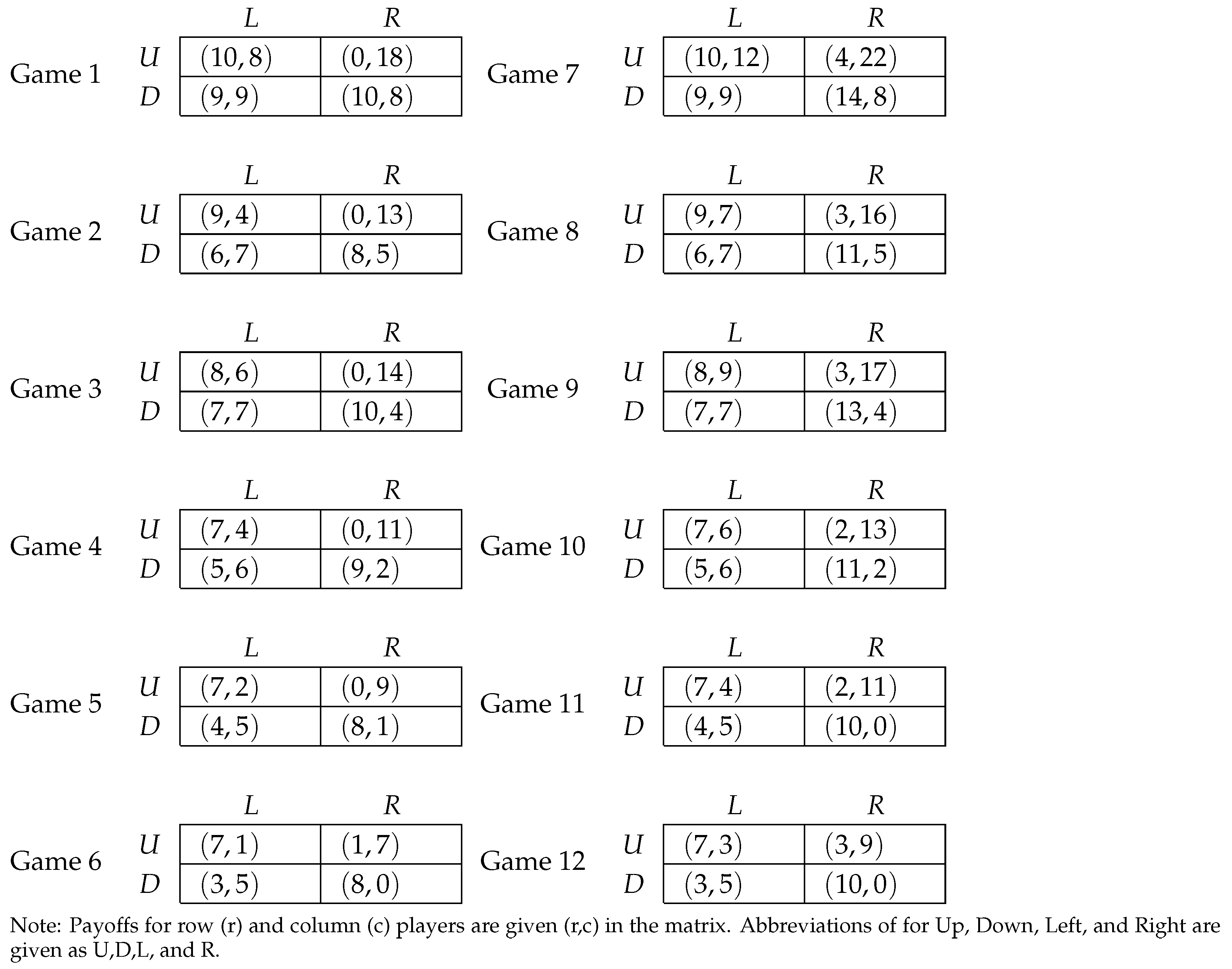
All of the games investigated are of the 2 × 2 form, as shown in Figure 1. The experiments from these games were collected by Selten and Chmura [8] and discussed in Chmura et al. [9]. Chmura et al. [9] investigate a series of learning models and determine which rules characterize individual and aggregate performance better. They find that self-tuning EWA fit the data best yet impulse-matching learning also fit the data well. The twelve 2 × 2 games include both constant sum and non-constant sum games.

The experiments were performed at the Bonn Lab with 54 sessions and 16 subjects in each session. 864 subjects participated in the experiment. The subjects in a given session were only exposed to one game. Games were 200 rounds long and subjects were randomly matched by round in groups of eight during the sessions. Knowledge of the game structure, payoffs, and matching protocols were public at the outset. The subject’s role of row or column player are fixed during the experiment, so four subjects in the group of eight were assigned to be a row player and the others were assigned to be a column player. At the end of each round, the subjects were told their current round payout, the other player’s choice, the round number, and their cumulative payout. The experiments lasted between 1.5 and 2 h and subjects received at 5 Euro show-up fee plus an average of 19 Euros in additional payouts.

5. Measuring Goodness of Fit

Following Chmura et al. [9], we use a quadratic scoring rule in order to assess the goodness of fit of each learning model.11 This rule, as described in Equation (13), provides a measure of nearness from the predicted choice to the observed choice.12

$$q_i\left(t\right)=2p_i\left(t\right)-{p_i\left(t\right)}^2-{(1-p_i\left(t\right))}^2$$

(13)

The quadratic score, $q_i\left(t\right)$, is a function of the probability, $p_i\left(t\right)$, of the choice by action i in period t. p is the predicted probability that is derived from the parameters of the learning models. The score is equal to 1 minus the squared distance between the predicted probability and the actual choice.

The expected range of $q_i\left(t\right)$ is $[-1,1]$. On one hand, if a learning model predicts the data perfectly, then $p_i\left(t\right)=1$, which implies $q_i\left(t\right)=1$. On the other hand, a completely uninformative learning model, in our setting, would be right half the time, so $p_i\left(t\right)=0.5$, which implies $q_i\left(t\right)=0.5$.

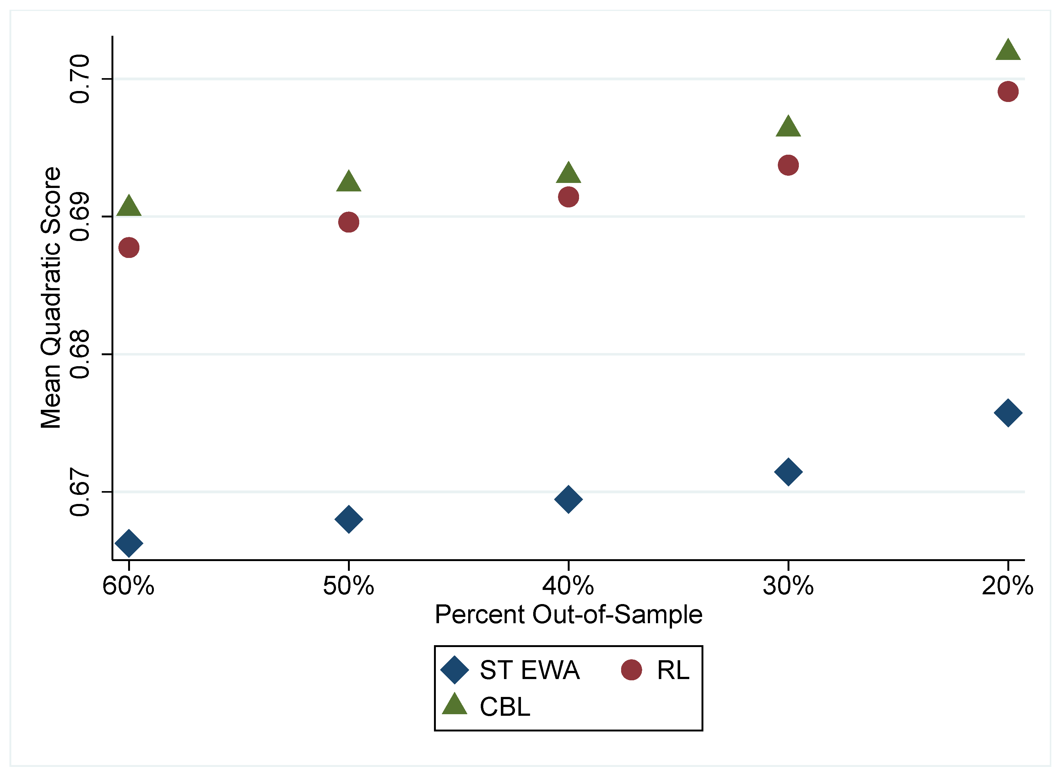
We employ the quadratic scoring rule in order to understand goodness of fit of each learning model in multiple tests. First, we calculate parameters on the entire playing history of all subjects and use the best-fitting parameters to estimate the predicted probabilities across playing history and calculate the mean quadratic score for each learning model. Next, we employ a rolling forward out-of-sample procedure. The out-of-sample process is chosen by fitting all models on the first $X\%$ of the data and using the fitted parameters of the model to predict the holdout sample of $(100-X)\%$ of the data. We then calculate the mean quadratic score for the remaining out-of-sample observations. We repeat for different values of X; in particular, we use 40%, 50%, 60%, 70%, and 80% in-sample training data to predict choice on the remaining 60%, 50%, 40%, 30%, and 20% remaining data, respectively. The in-sample method is a standard way to judge goodness-of-fit, by simply looking at how much of the whole data the model can explain individual choice. The out-of-sample method guards against over-fitting the data, but, to be valid, it assumes stationarity of parameters across the in-sample and holdout data. For concerns of over-fitting the data with any learning model, this out-of-sample procedure is the preferred benchmark in choosing which model explain the data best.

In estimating CBL, we use information available to subjects to define the Problem set $\mathcal{P}$. In our main specification, we choose two elements in the information vector (i.e., problem vector). The first element is the round of the game (i.e., time). The round of the game plays the role of recency, or forgetting, in other learning models; cases that are distant in the past are less similar to present circumstances than cases that happened more recently. The second element is the opponents’ play from the game. We account for other players actions by using a moving average of past play, treating all opponents as a representative player, just as we do for the surprise index in self-tuning EWA. We use a four period moving average. For example, a row player would use the moving average of how many times their opponents played Left as a component of similarity and, as opponents trend toward different frequencies of playing Left, the CBL would put less weight on those cases, $\mathcal{C}$. There are many possible choices on how to incorporate these information vectors and we explore them further in the Appendix B in

Table A1. Information Vector Definitions.

	(1)
	Mean Quadratic Score
One lag	0.677
Two lags	0.684
Three lags	0.682
MA-3	0.678
MA-5	0.678

Note: Each lag represents a extra parameter on whether a partner in the past played either Up or Left, depending on the roll of the subject. Abbreviations: MA-3 moving average for past three rounds, MA-5 moving average for past five rounds.

. We find that these choices do not have a large effect on the performance of CBL.

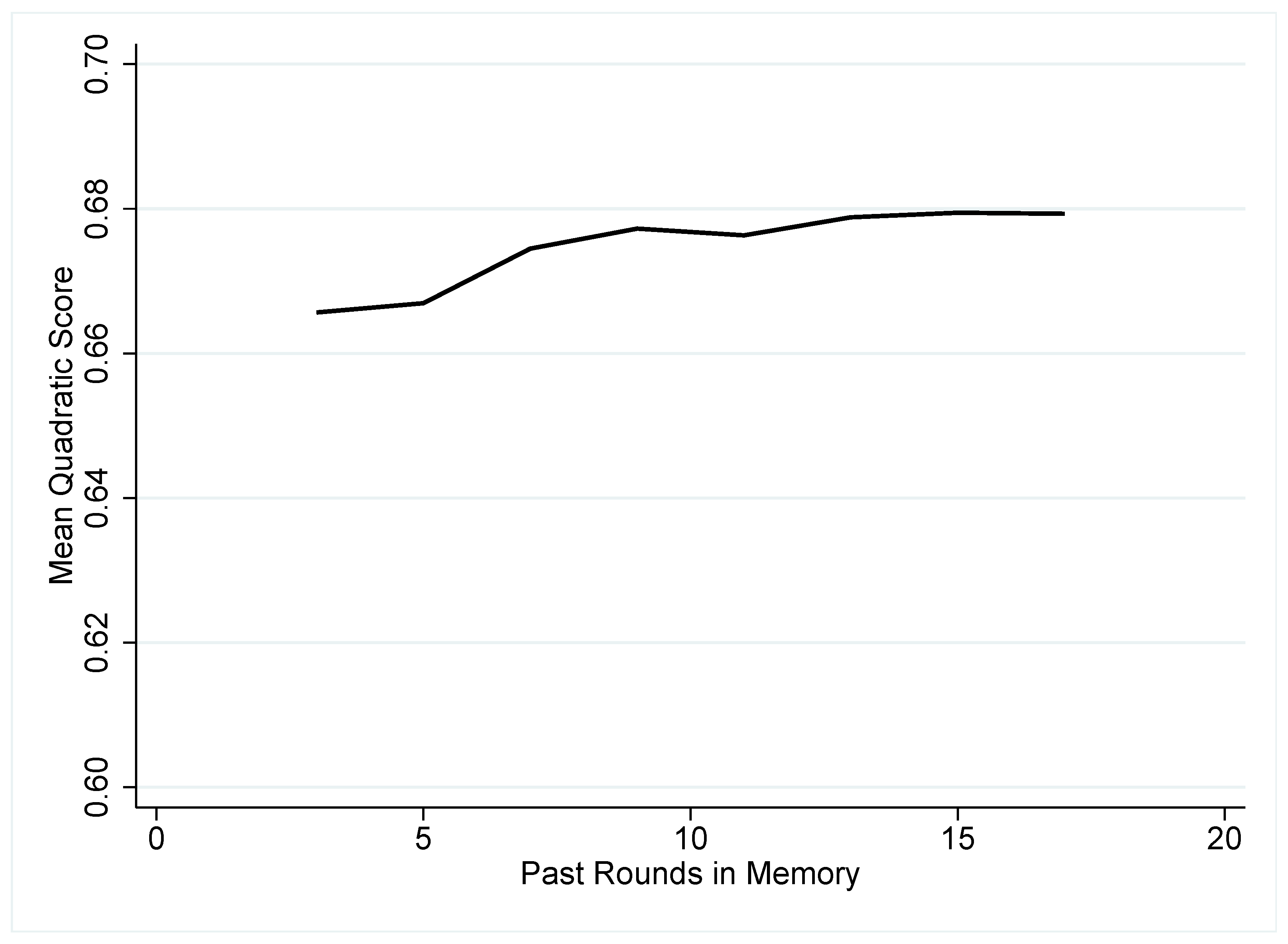
We include cases as much as 15 periods in the past in memory (we explore the sensitivity of this assumption in Section 7.1).

6. Results

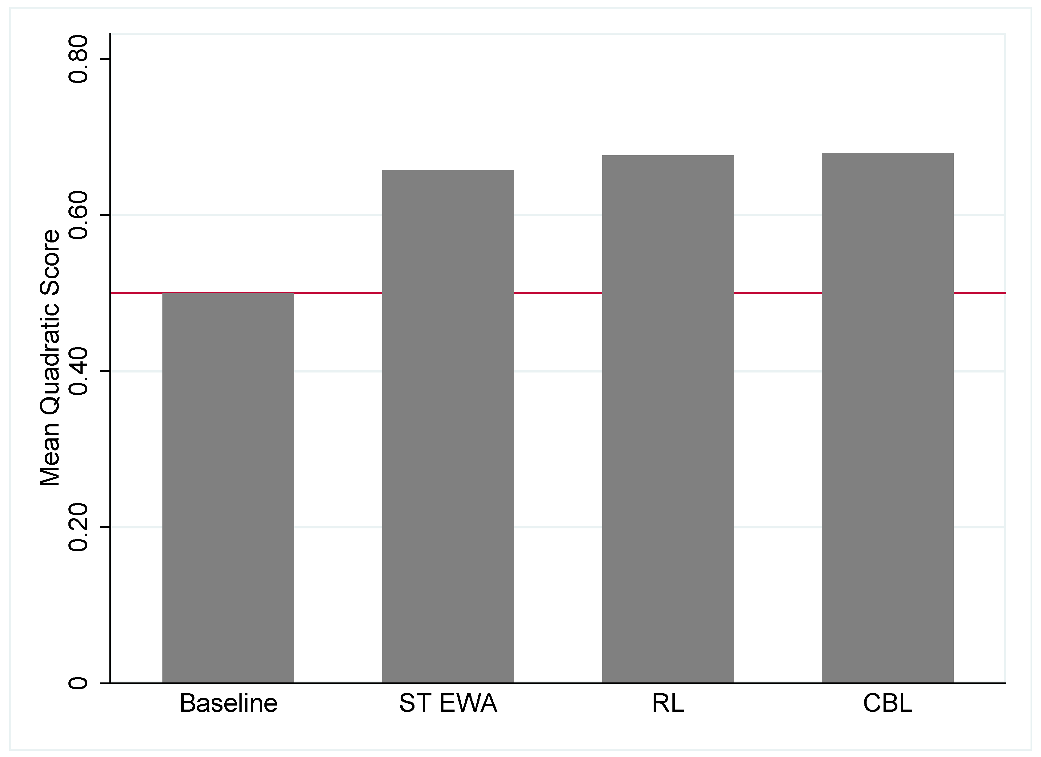
To fit the learning models to data, we estimate Equation (2) for CBL, Equation (5) for RL, and Equation (6) for self-tuning EWA. All of the learning algorithms use the stochastic logit choice rule in Equation (12). In Figure 2, we report the mean quadratic score by the learning models discussed in the previous section across all 12 experimental games. We find when using in-sample measures between the learning models that CBL fits best, RL fits second best, and self-tuning EWA fits third best.13 RL performs about as well as CBL across these experimental games. As expected, each learning model outperforms a baseline benchmark of random choice (i.e., a mean quadratic score of 0.5). Note that Chmura et al. [9] also find that self-tuning EWA and a selection of other simple learning models out-perform random choice, but they found self-tuning EWA was the best performing learning model in predicting individual choice with these data.14

We use a non-nested model selection test proposed by Vuong [40], which provides a directional test of which model is favored in the data generating process. Testing the CBL model versus the RL model, the Vuong test statistic is 7.45, which is highly significant and favors the selection of the CBL model. In addition, we find that the CBL is selected over the ST EWA model with a Voung test statisitic of 37.91.

In Figure 3, we report the mean quadratic scores of the out-of-sample data using in-sample parameter estimates. We find similar conclusions as in the in-sample fit in Figure 2. CBL fits best, followed by RL, and then by ST EWA. This leads us to presume that CBL may be better at explaining behavior across all these games, likely due to the inclusion of information about the moving average of opposing players’ play during the game. It is important to note that the RL predicts almost as well as CBL with arguably a simpler learning model. The experiments we use, and have been traditionally used to assess learning models, are relatively information-poor environments for subjects compared to some other games. For example, many one-shot prisoner dilemma games or coordination games where information about partner’s identity or their past play is public knowledge would be a comparably information-rich environment. This makes us optimistic that CBL may be even more convincing in information-rich environments. Because CBL makes use of the data about opposing players, CBL is an obvious candidate to accommodate this type of information in a systematic way that seems consistent with the psychology of decision making.

7. Case-Based Parameters

In this section, we discuss the parameters of CBL estimation based on the full sample estimation. The parameters of CBL are $\lambda$, which measures the sensitivity of choice to CBU (see Section 3.6), $A_0^L$ is the parameter measuring the initial attraction for Left for the column player, while $A_0^U$ is the initial attraction for Up for the row player (see Section 3.1). These initial attractions are relative measures as the initial attractions for Down and Right are held at zero. $W_i$ are weights in the similarity function on the different characteristics of the information vector (see Equation (4)). In particular, $W_1$ is the weight given to recency (here, round number), $W_2$ is the weight given to the moving average of actions of opposing players. These parameters are estimated to best fit the data using the logit rule in Equation (12).

We do not directly estimate the aspiration parameter, because it cannot be effectively empirically distinguished from the initial attraction parameters. If one considers Equation (2), one can see that the H parameter and the mean of the $A_j$ parameters confound identification. We cannot distinguish between the average initial attractions to strategies due to priors and the aspiration value of the agent. Fortunately, we find that the fit of the CBL generally does not rely on the estimation of the aspiration level to achieve the same goodness-of-fit.

In

Table 1. CBL Parameter Estimates. Note: ***, **, * denote statistical significance of 10%, 5%, and 1%. Clustered standard errors by subject are in parentheses. MQS is the mean quadratic score. ${}^{†}$ The standard error did not calculate using clustered standard errors and is instead calculated using the outer product of the gradient (OPG) vectors method.

	A: Combined Models
	$\mathit{\lambda }$	${\mathit{A}}_{\mathbf{0}}^{\mathit{L}}$	${\mathit{A}}_{\mathbf{0}}^{\mathit{U}}$	${\mathit{W}}_{\mathbf{1}}$	${\mathit{W}}_{\mathbf{2}}$	N	MQS
Constant sum games	10.896 ***	−1.596 ***	1.775 ***	0.043 ***	15.917 ***	115,200	0.688
	(0.331)	(0.211)	(0.250)	(0.002)	(0.002)
Non-constant sum games	37.831 ***	−1.024 ***	1.023 ***	1.136 ***	10.259 ***	57,600	0.653
	(1.748)	(0.148)	(0.143)	(0.000)	(1.006) ${}^{†}$
All games	10.179 ***	−1.946 ***	1.553 ***	0.049 ***	9.365 ***	172,800	0.679
	(0.186)	(0.195)	(0.204)	(0.000)	(0.364) ${}^{†}$
	B: Individual Game Models
	$\mathit{\lambda }$	${\mathit{A}}_{\mathbf{0}}^{\mathit{L}}$	${\mathit{A}}_{\mathbf{0}}^{\mathit{U}}$	${\mathit{W}}_{\mathbf{1}}$	${\mathit{W}}_{\mathbf{2}}$	N	MQS
Game 1	15.543 ***	−1.397 ***	4.821 ***	0.205 ***	4.146 ***	19,200	0.809
	(0.823)	(0.437)	(1.021)	(0.016) ${}^{†}$	(0.953) ${}^{†}$
Game 2	6.655 ***	−0.730 *	2.395 **	0.019 ***	5.316 ***	19,200	0.667
	(0.925)	(0.444)	(1.179)	(0.007)	(1.376)
Game 3	15.175 ***	−1.753	2.465 ***	0.127	3.929 ***	19,200	0.768
	(0.584) ${}^{†}$	(3.794)	(0.269) ${}^{†}$	(0.134)	(0.398)
Game 4	13.758 ***	−2.683 ***	2.139 ***	0.139 ***	3.167 ***	19,200	0.654
	(0.832)	(0.471)	(0.352)	(0.005)	(0.028)
Game 5	110.704 ***	−0.416 ***	0.377 ***	3.204 ***	7.261 ***	19,200	0.630
	(8.723)	(0.071)	(0.078)	(0.000)	(2.352) ${}^{†}$
Game 6	65.058 ***	−0.406 ***	0.114	1.535 ***	3.246 **	19,200	0.594
	(5.276)	(0.125)	(0.090)	(0.003)	(1.507) ${}^{†}$
Game 7	33.815 ***	−0.431	2.135 ***	1.005 ***	8.853 ***	9600	0.741
	(3.764)	(0.316)	(0.618)	(0.104) ${}^{†}$	(0.875)
Game 8	5.300 *	−3.121 **	3.856 **	0.020	5.155 *	9600	0.637
	(3.092)	(1.475)	(1.941)	(0.041)	(2.783)
Game 9	10.058 ***	−4.345 ***	2.512 ***	0.080 ***	2.784 ***	9600	0.743
	(0.724)	(1.155)	(0.695)	(0.000)	(0.004)
Game 10	5.837 ***	−4.364 **	−0.563	0.020 ***	1.499 ***	9600	0.639
	(0.836)	(2.063)	(1.025)	(0.008)	(0.013)
Game 11	20.525 ***	−1.588 ***	1.444 ***	0.394 ***	0.767 ***	9600	0.616
	(1.638)	(0.487)	(0.416)	(0.000)	(0.004)
Game 12	7.184 ***	−1.864	0.604	0.012 **	8.471 ***	9600	0.593
	(1.078)	(1.162)	(0.890)	(0.005)	(2.254)

, we report the estimated parameters using the full sample of observations in each treatment of each experiment. In all experimental treatments, we find a statistically significant value for $\lambda$, meaning that the learning algorithm estimated explains some choice. We find that the initial attraction parameters $A_0^j$ are consistent with the frequency of choices in the first period. The relative weights of $W_1$ and $W_2$ are difficult to directly compare, as they are in different scales. We could normalize the data prior to estimation, but it is unclear what affect that might have on cumulative CBL over time. We explore ex-post normalization of the parameters in Appendix C and list results in

Table A2. CBL Normalized weights.

	${\mathit{W}}_1$	${\mathit{W}}_2$
Constant sum games	0.544	2.435
Non-constant sum games	14.245	1.539
All games	0.622	1.414

. The empirical estimate of $W_1$ is positive and statistically significant. This indicates that, consistent with other learning models, recency is important to learning.

By comparing the coefficients $W_1$ in Table 1, we find that recency degrades similarity faster in non-constant sum games than in constant sum games. This difference suggests that in non-constant sum game, subjects ’forget’ past experience faster when constructing expectations about the current problem and they put relatively more weight on the similarity of the moving average of opposing players.

The weight, $W_2$, on the moving average of past play of opposing players is positive and significant. A positive parameter gives greater weight to cases with similar average playing rates to the current problem. This parameter picks up adjustments to group actions over time.

7.1. Memory

We explore to what extent adding memory explains behavior in CBL. This is an important part of our depiction of learning, and we test the regularity to which it is important by varying the known memory of subjects in CBL. Figure 4 shows the improvement in the mean quadratic score as more memory is allowed in the CBL algorithm starting with three prior periods in memory ($M=3$) and expanding to seventeen prior periods ($M=17$). If we refer to three periods in memory, then subjects ‘forget’ periods that were further in the past than three periods (rounds) ago and do not consider them in comparing the current periods definition of a case. The figure demonstrates that increasing the length of short time-horizons provide an improvement in model fit, but most gains are exhausted by around nine periods. Because period number is included as an element of the problem definition $\mathcal{P}$, continuing to add more periods into the similarity function makes little difference past nine periods and degrades past fifteen periods. This provides the basis of our choice of fifteen periods for estimation.

7.2. Definition of Similarity

We estimate multiple similarity functional forms and measures of distance between the attributes used in the definition similarity between problems. We test how similarity as characterized by Equation (14) compares to in-sample fit of the data. The definitions of our similarity functions primarily differ in how similarity decays; above, we assume similarity decays exponentially and, in Equation (14), it decays according to the logarithm (Ones were added to avoid dividing-by-zero and log-of-zero problems).

$$S^2(x,y)=\frac{1}{ln\left(d(x,y)+1\right)+1}$$

(14)

In addition to the decay of similarity, we can also test a different definition of distance between elements of the problem. In our main specification, we use weighted Euclidean distance, as defined in Equation (4). Another popular definition in psychology for distance is the Manhattan distance given by Equation (15).

$$\begin{array}{ccc}\hfill d^2(x,y)& =& {\displaystyle \sum _{i=1}^{\#Dims}{w}_i|x_i-y_i|}\hfill \end{array}$$

(15)

Using these definitions, we report that the in-sample fit of the data, measured by the quadratic scoring rule, in Table 1 to be robust to the various definitions of similarity and distance. We indicate by column heading in

Table 2. Similarity Definitions Measured by Mean Quadratic Score.

	(1)	(2)	(3)	(4)
	$\mathit{S}$, $\mathit{d}$	${\mathit{S}}^{\mathbf{2}}$, $\mathit{d}$	$\mathit{S}$, ${\mathit{d}}^{\mathbf{2}}$	${\mathit{S}}^{\mathbf{2}}$, ${\mathit{d}}^{\mathbf{2}}$
MQS	0.679	0.686	0.681	0.682

Note: S denotes the similarity function in Equation (3) and $S^2$ denotes the similarity function in Equation (4). d denotes the Euclidean distance function and $d^2$ denotes the Manhattan distance function.

which equations were used corresponding to specific functional forms of similarity and distance. The functional form of distance between elements seems to be of minor importance to fit in the mixed strategy equilibria games explored here. Nevertheless, there is greater variation in the performance of the different similarity functions. The similarity function provided in Equation (14) performs better than the exponential. We also find the weight $W_2$ with Equation (14) is negative and statistically significant, which is unexpected. To avoid overfitting the data with parameters that do not make psychological sense, we use Equation (3) in our main specification. We conclude that CBL is robust to different definitions of similarity, and the inverse exponential function is a good fit with the experimental data at hand. This also corresponds to previous findings in psychology and economics [4,33].

8. Empirical Comparison of Learning Models

In this section, we investigate the dynamics of RL and CBL, the two best-fitting learning models, to more fully understand the results of these learning algorithms. Previously we discussed the potential overlap in RL and CBL, which in practice have similar fits to the data. CBL likely outperforms RL in aggregate due to its ability to incorporate important information in the the choice behavior of subjects. RL and CBL appear to converge on choices overtime. We illustrate convergence in prediction between CBL and RL in Figure 5. There is a possibility that RL and CBL are increasingly correct about different types of individual decisions and could not actually be converging to similar predictions of behavior. For example, say there are three types of decision makers (A, B, and C). CBL and RL predict players of type A well, but not B or C. As more information is added and the learning models improve goodness of fit, CBL predicts player type B better and RL predicts player type C better. Both of the models are doing better, but are doing it on different observations and therefore on not converging on the types of predictions they get correct. The convergence between CBL and EWA by round in Figure 5 demonstrates that the gains in accuracy are accompanied by a convergence in agreement between the two learning algorithms, although convergence is slight. The coefficient of the regression line in Figure 5 is −0.00006 with a clustered standard error by game type of 0.00002. This coefficient is statistically significant with a t-statistic of −2.98.

We also provide the model fits by individual games in Appendix D.

Table A3. In-sample Fit by Game: Mean Quadratic Score * denotes the best-fitting model based on the mean quadratic score. CBL has five estimated parameters, RL has four estimated parameters, and ST EWA has one estimated parameter. ST EWA refers to the self-tuning EWA, RL refers to reinforcement learning, and CBL refers to case-based learning.

	CBL	ST EWA	RL
Game 1	0.809 *	0.785	0.808
Game 2	0.667 *	0.661	0.667
Game 3	0.768 *	0.750	0.767
Game 4	0.654 *	0.636	0.650
Game 5	0.630	0.608	0.633 *
Game 6	0.594	0.568	0.598 *
Game 7	0.741	0.735	0.751 *
Game 8	0.637 *	0.629	0.636
Game 9	0.743 *	0.706	0.738
Game 10	0.639 *	0.607	0.637
Game 11	0.616 *	0.597	0.615
Game 12	0.593 *	0.573	0.590

and

Table A4. Out-of-sample Fit by Game Note: * denotes the best fitting model based on the mean quadratic score. ST EWA refers to the self-tuning EWA, RL refers to reinforcement learning, and CBL refers to case-based learning.

	A: Out-of-Sample: Predict Last 60%			B: Out-of-Sample: Predict Last 50%
	CBL	ST EWA	RL	CBL	ST EWA	RL
Game 1	0.827	0.811	0.838 *	0.845 *	0.817	0.844
Game 2	0.674	0.669	0.675 *	0.671	0.671	0.677 *
Game 3	0.793 *	0.771	0.793	0.782	0.778	0.798 *
Game 4	0.658 *	0.637	0.653	0.659 *	0.637	0.655
Game 5	0.636 *	0.607	0.632	0.641 *	0.607	0.634
Game 6	0.601 *	0.568	0.600	0.603 *	0.567	0.599
Game 7	0.768	0.766	0.783 *	0.784	0.769	0.785 *
Game 8	0.641	0.638	0.644 *	0.637	0.637	0.642 *
Game 9	0.743	0.715	0.747 *	0.746	0.711	0.747 *
Game 10	0.632	0.605	0.638 *	0.645 *	0.610	0.641
Game 11	0.616	0.598	0.617 *	0.618	0.601	0.624 *
Game 12	0.593 *	0.576	0.593	0.579	0.574	0.593
	C: Out-of-Sample: Predict Last 40%			D: Out-of-Sample: Predict Last 30%
	CBL	ST EWA	RL	CBL	ST EWA	RL
Game 1	0.843	0.818	0.847	0.854	0.82	0.852
Game 2	0.665	0.672	0.680 *	0.669	0.671	0.680 *
Game 3	0.787	0.779	0.800 *	0.792	0.780	0.802 *
Game 4	0.661 *	0.636	0.655	0.664 *	0.641	0.659
Game 5	0.641 *	0.607	0.634	0.643 *	0.611	0.635
Game 6	0.594	0.569	0.600 *	0.606 *	0.574	0.603
Game 7	0.789	0.775	0.792 *	0.791	0.777	0.795 *
Game 8	0.635	0.635	0.640 *	0.639	0.634	0.639 *
Game 9	0.750 *	0.715	0.748	0.737	0.714	0.748 *
Game 10	0.651 *	0.613	0.650	0.643	0.614	0.651 *
Game 11	0.621	0.605	0.626 *	0.621	0.603	0.624 *
Game 12	0.596 *	0.574	0.594	0.599	0.579	0.599 *
	E: Out-of-Sample: Predict Last 20%
Game 1	0.866 *	0.821	0.862
Game 2	0.694	0.686	0.697 *
Game 3	0.804	0.789	0.806 *
Game 4	0.660	0.642	0.661 *
Game 5	0.637 *	0.612	0.636
Game 6	0.609 *	0.574	0.604
Game 7	0.794 *	0.776	0.794
Game 8	0.634	0.637	0.643 *
Game 9	0.746	0.726	0.757 *
Game 10	0.663	0.626	0.666 *
Game 11	0.620	0.608	0.629 *
Game 12	0.591	0.575	0.595 *

show the in-sample and out-of-sample model fits by individual game for all learning models.

9. Discussion

The parameters of CBL are also related to other theories of learning. Aspiration levels can be incorporated into both the self-tuning EWA and CBL models of learning. They are somewhat inherent in the self-tuning EWA algorithm already because the attractions compare the average payoffs of previous attractions to the the current attraction and act as an endogenous version of aspiration level that incorporates foregone payoffs. Another similarity between these theories of behavior is recency, or the weighting of events that have more recently occurred in the past. In self-tuning EWA and RL, the parameter $\varphi$ and cumulative attractions account for recency and, in CBL, a time indicator in the definition of the problem and definition of memory account for recency. In all the learning models, recency allows individuals to ’forget’ old occurrences of a problem and adapt to new emergent behavior or payoffs.

In this study, we show the effectiveness of CBL in an environment used traditionally for learning models. CBL can easily be applied to other contexts with the same basic construction showed here. It would be simple to estimate the same algorithm on other games through the same procedures or choice data from outside the lab. The harder question is how to define the Problem, $\mathcal{P}$, in these different environments. In Appendix B, we discuss different definitions of the Problem for this context. We find the results aree robust to the definition of Problem in Table A1. In more information-rich contexts, it may be difficult to decide the number of characteristics, how information is presented in the similarity function, and whether fictitious cases are present in memory. One approach, if experiments are used, could be to track attention to particular pieces of information (e.g., through mouse clicks, eyetracking, or even asking subjects). Collecting secondary information on choices may be beneficial testing axioms of case-based decision theory. Further, as in Bleichrodt et al. [17], through experimental design, decision weights for information can be constructed to further understand the properties of CBL that can be non-parametrically estimated.

One suggested limitation of learning models is that they do not explain why the way partners are matched matters [41], although more sophisticated learners can address this deficiency [32]. CBL may better explain why matching matters directly through the information vector and the similarity function. This is the biggest difference between CBL and other algorithms: the formulation of how information enters into decision making, which is systematic, follows what we know from psychology about decision making of individuals, and it is shown to be important through numerous experimental investigations.

CBL also has the ability to incorporate fictitious play, although we do not pursue this in the current paper. As mentioned above, although typically an agent’s memory is the list of cases she has experienced—which is what we assume here—it is possible for cases in memory to come from some other sources. The agent could add fictitious play cases to memory and thereafter use those fictitious cases to calculate CBL. Moreover, this agent could distinguish fictitious from real cases if she so desired by adding a variable to the information vector denoting whether the case was fictitious; then fictitious cases could have less—but not zero—importance relative to real cases. Bayesian learning can also be tractable in the case of 2 × 2 games, where the dimensions of the state space are small. We did not consider forgone payoffs in CBL and, therefore, did not compare CBL to other Belief models. We can imagine that comparing CBL to Bayesian learning models that would have priors defined over the complete state space is a natural next step in this line of research. We leave this for future investigation.

10. Conclusions

In this work, we demonstrate the estimation of a new learning model based on an existing decision theory, Case-based Decision Theory. This form of decision-making under uncertainty when applied to game theoretic experiments performs well when compared to two other leading learning models: Reinforcement Learning and self-tuning Experience Weighted Attraction. An important feature of Case-Based Learning is the ability to systematically incorporate information that is available to subjects into choice decisions. Real people condition their behavior on their observations of their environments, and the case-based approach incorporates this in a natural way.

The parameters of Case-Based Learning indicate a relationship between recency and the type of game played. Constant sum games exhibit a smaller recency effect than non-constant sum games. This indicates that subjects weight experience with a opponents differently, depending on the type of game played. Significant attention is given to the average rates of play, and changes to those average rates of play, through the inclusion of moving averages in the definition of the ‘Problem’.

Further work in applying CBL to other decision making environments is important in understanding its limits and sensible parameterizations of information vectors, hypothetical references, and how deliberate thoughtful decisions are affected by institutions that include information. CBL could also be used and adapted to predict behavior across different types of games, or more generally changes to decision-making environments, to understand the influence of previous game play on decisions in new environments and how subjects encode information across games. A natural extension of this type of investigation are repeated prisoner dilemma games or repeated coordination games, which allow more complex equilibria, but also allow for a greater freedom to explore the primitives of learning across environments.

References

- Gilboa, I.; Schmeidler, D. Case-based decision theory. Q. J. Econ. 1995, 110, 605–639. [Google Scholar] [CrossRef] [Green Version]
- Von Neumann, J.; Morgenstern, O. Theory of Games and Economic Behavior; Princeton University Press: Princeton, NJ, USA, 1944. [Google Scholar]
- Savage, L.J. The Foundations of Statistics; Wiley: New York, NY, USA, 1954. [Google Scholar]
- Pape, A.D.; Kurtz, K.J. Evaluating case-based decision theory: Predicting empirical patterns of human classification learning. Games Econ. Behav. 2013, 82, 52–65. [Google Scholar] [CrossRef]
- Guilfoos, T.; Pape, A.D. Predicting human cooperation in the Prisoner’s Dilemma using case-based decision theory. Theory Decis. 2016, 80, 1–32. [Google Scholar] [CrossRef]
- Luce, R.D. Individual Choice Behavior; Dover Publications Inc.: Menola, NY, USA, 1959. [Google Scholar]
- Erev, I.; Roth, A.E. Predicting how people play games: Reinforcement learning in experimental games with unique, mixed strategy equilibria. Am. Econ. Rev. 1998, 88, 848–881. [Google Scholar]
- Selten, R.; Chmura, T. Stationary concepts for experimental 2 × 2-games. Am. Econ. Rev. 2008, 98, 938–966. [Google Scholar] [CrossRef]
- Chmura, T.; Goerg, S.J.; Selten, R. Learning in experimental 2 × 2 games. Games Econ. Behav. 2012, 76, 44–73. [Google Scholar] [CrossRef] [Green Version]
- Ho, T.H.; Camerer, C.F.; Chong, J.K. Self-tuning experience weighted attraction learning in games. J. Econ. Theory 2007, 133, 177–198. [Google Scholar] [CrossRef] [Green Version]
- Gayer, G.; Gilboa, I.; Lieberman, O. Rule-based and case-based reasoning in housing prices. BE J. Theor. Econ. 2007, 7. [Google Scholar] [CrossRef] [Green Version]
- Kinjo, K.; Sugawara, S. Predicting empirical patterns in viewing Japanese TV dramas using case-based decision theory. BE J. Theor. Econ. 2016, 16, 679–709. [Google Scholar] [CrossRef]
- Golosnoy, V.; Okhrin, Y. General uncertainty in portfolio selection: A case-based decision approach. J. Econ. Behav. Organ. 2008, 67, 718–734. [Google Scholar] [CrossRef] [Green Version]
- Guerdjikova, A. Case-based learning with different similarity functions. Games Econ. Behav. 2008, 63, 107–132. [Google Scholar] [CrossRef]
- Ossadnik, W.; Wilmsmann, D.; Niemann, B. Experimental evidence on case-based decision theory. Theory Decis. 2013, 75, 1–22. [Google Scholar] [CrossRef]
- Grosskopf, B.; Sarin, R.; Watson, E. An experiment on case-based decision making. Theory Decis. 2015, 79, 639–666. [Google Scholar] [CrossRef] [Green Version]
- Bleichrodt, H.; Filko, M.; Kothiyal, A.; Wakker, P.P. Making case-based decision theory directly observable. Am. Econ. J. Microecon. 2017, 9, 123–151. [Google Scholar] [CrossRef]
- Radoc, B.; Sugden, R.; Turocy, T.L. Correlation neglect and case-based decisions. J. Risk Uncertain. 2019, 59, 23–49. [Google Scholar] [CrossRef] [Green Version]
- Bhui, R. Case-Based Decision Neuroscience: Economic Judgment by Similarity. In Goal-Directed Decision Making; Elsevier: Amsterdam, The Netherlands, 2018; pp. 67–103. [Google Scholar]
- Gayer, G.; Gilboa, I. Analogies and theories: The role of simplicity and the emergence of norms. Games Econ. Behav. 2014, 83, 267–283. [Google Scholar] [CrossRef]
- Bordalo, P.; Gennaioli, N.; Shleifer, A. Memory, Attention, and Choice. Q. J. Econ. 2020, 135, 1399–1442. [Google Scholar] [CrossRef]
- Argenziano, R.; Gilboa, I. Similarity & Nash Equilibria in Statistical Games. Available online: https://www.researchgate.net/publication/334635842_Similarity-Nash_Equilibria_in_Statistical_Games (accessed on 23 July 2019).
- Gilboa, I.; Lieberman, O.; Schmeidler, D. Empirical Similarity. Rev. Econ. Stat. 2006, 88, 433–444. [Google Scholar] [CrossRef]
- Billot, A.; Gilboa, I.; Schmeidler, D. Axiomatization of an Exponential Similarity Function. Math. Soc. Sci. 2008, 55, 107–115. [Google Scholar] [CrossRef] [Green Version]
- Matsui, A. Expected Utility and Case-Based Reasoning. Math. Soc. Sci. 2000, 39, 1–12. [Google Scholar] [CrossRef]
- Charness, G.; Gneezy, U. What’s in a name? Anonymity and social distance in dictator and ultimatum games. J. Econ. Behav. Organ. 2008, 68, 29–35. [Google Scholar] [CrossRef] [Green Version]
- Guilfoos, T.; Kurtz, K.J. Evaluating the role of personality trait information in social dilemmas. J. Behav. Exp. Econ. 2017, 68, 119–129. [Google Scholar] [CrossRef] [Green Version]
- Cerigioni, F. Dual Decision Processes: Retrieving Preferences When Some Choices are Intuitive; Economics Working Papers; Department of Economics and Business, Universitat Pompeu Fabra: Barcelona, Spain, 2016. [Google Scholar]
- Fudenberg, D.; Levine, D.K. The Theory of Learning in Games; MIT Press: Cambridge, MA, USA, 1998; Volume 2. [Google Scholar]
- Camerer, C.; Ho, T.H. Experience-weighted attraction learning in coordination games: Probability rules, heterogeneity, and time-variation. J. Math. Psychol. 1998, 42, 305–326. [Google Scholar] [CrossRef] [PubMed] [Green Version]
- Camerer, C.; Ho, T.H. Experience-weighted attraction learning in normal form games. Econometrica 1999, 67, 827–874. [Google Scholar] [CrossRef] [Green Version]
- Camerer, C.F.; Ho, T.H.; Chong, J.K. Sophisticated experience-weighted attraction learning and strategic teaching in repeated games. J. Econ. Theory 2002, 104, 137–188. [Google Scholar] [CrossRef] [Green Version]
- Shepard, R. Toward a Universal Law of Generalization for Psychological Science. Science 1987, 237, 1317. [Google Scholar] [CrossRef] [Green Version]
- Dayan, P.; Niv, Y. Reinforcement learning: The good, the bad and the ugly. Curr. Opin. Neurobiol. 2008, 18, 185–196. [Google Scholar] [CrossRef]
- Glimcher, P.W. Understanding dopamine and reinforcement learning: The dopamine reward prediction error hypothesis. Proc. Natl. Acad. Sci. USA 2011, 108, 15647–15654. [Google Scholar] [CrossRef] [Green Version]
- Harley, C.B. Learning the evolutionarily stable strategy. J. Theor. Biol. 1981, 89, 611–633. [Google Scholar] [CrossRef]
- Roth, A.E.; Erev, I. Learning in extensive-form games: Experimental data and simple dynamic models in the intermediate term. Games Econ. Behav. 1995, 8, 164–212. [Google Scholar] [CrossRef]
- Brier, G.W. Verification of forecasts expressed in terms of probability. Mon. Weather Rev. 1950, 78, 1–3. [Google Scholar] [CrossRef]
- Selten, R. Axiomatic characterization of the quadratic scoring rule. Exp. Econ. 1998, 1, 43–61. [Google Scholar] [CrossRef]
- Vuong, Q.H. Likelihood ratio tests for model selection and non-nested hypotheses. Econom. J. Econom. Soc. 1989, 57, 307–333. [Google Scholar] [CrossRef] [Green Version]
- Andreoni, J.; Miller, J.H. Rational cooperation in the finitely repeated prisoner’s dilemma: Experimental evidence. Econ. J. 1993, 103, 570–585. [Google Scholar] [CrossRef]