Homogenous Granulation and Its Epsilon Variant ^†

Abstract

In the era of Big data, there is still place for techniques which reduce the data size with maintenance of its internal knowledge. This problem is the main subject of research of a family of granulation techniques proposed by Polkowski. In our recent works, we have developed new, really effective and simple techniques for decision approximation, homogenous granulation and epsilon homogenous granulation. The real problem in this family of methods was the choice of an effective parameter of approximation for any datasets. It was resolved by homogenous techniques. There is no need to estimate the optimal parameters of approximation for these methods, because those are set in a dynamic way according to the data internal indiscernibility level. In this work, we have presented an extension of the work presented at ICIST 2018 conference. We present results for homogenous and epsilon homogenous granulation with the comparison of its effectiveness.

1. Introduction

Granular rough computing is one of the techniques used for decision system approximation. This method relies on knowledge granules which are formed from objects with selected, similar features. The main goal is to reduce the amount of data being used for classification or regression, maintaining internal knowledge of the decision system. In the era of processing large datasets these techniques can play a significant role. Basic granulation methods were proposed by Polkowski [1,2]. In the works of Artiemjew [3,4], Polkowski [1,2,5,6,7,8], and Polkowski and Artiemjew [9,10,11,12,13,14] we have presented standard granulation, concept dependent and layered granulation in the context of data reduction, missing values absorbtion and usage in the classification process.

Our motivation to perform this research was an idea to determine effective indiscernibility ratio of decision system approximation without its estimation. The ratio of approximation has influence on the original data size reduction. In our previous methods. we had to estimate this parameter reviewing the set of radii from 0 to 1. In the methods proposed in this work, we do not have to perform this operation. The ratio, for particular central object, is chosen in an automatic way, by extending it until the set of objects is homogenous in the sense of belonging to the decision class. Instead of performing granulation several times, depending on the number of attributes of the object, this process is performed only once, solving the problem of optimal radii search. Our results are showing reduction of training dataset size by up to 50 percent maintaining the internal knowledge at a satisfying level which was measured by efficiency of the classification process. The method is simple, has a square time complexity, $U^2$ main operations time the scalar $\left|A\right|$. U is the set of objects of decision system, A the set of conditional attributes.

In this work, we have described the results of our previous research, presented in detail in [15,16]. The results are prepared for nominal (Homogenous granulation) data and numerical data (Epsilon homogenous granulation). It is worth to mention that our new methods were implemented in really effective new ensemble model; see [17].

The paper has the following content. In Section 2 there is a theoretical background. In Section 3 and Section 4 we present a description of a our granulation techniques. In Section 5 we present a description of a classifier used in the experimental part. In Section 6 there are the results of our experiments and the conclusion is presented in Section 7.

There are three basic steps of the granulation process. The granules are computed for each training object, then, the training dataset is covered using the selected strategy and in the last step, majority voting is being used to get granular reflection of the training system.

In the next section, we describe the first step of the mentioned procedure.

2. Granular Rough Inclusions

Some more theory about rough inclusions can be found in Polkowski [1,6,7,18,19], a detailed discussion may be found in Polkowski [8].

For given objects u and v from training decision system $U,A,d$, where U is the universe of objects, A the set of conditional attributes, and d is the decision attribute. The standard rough inclusion $\mu$ is defined as

$$\mu (v,u,r)\iff \frac{\left|IND\right(u,v\left)\right|}{\left|A\right|}\ge r$$

(1)

where

$$IND(u,v)=\{a\in A:a(u)=a(v)\},$$

(2)

The parameter r is the granulation radius from the set $\{0,\frac{1}{\left|A\right|},\frac{2}{\left|A\right|},\dots ,1\}$.

2.1. $\epsilon$–Modification of the Standard Rough Inclusion

Given a parameter $\epsilon$ valued in the unit interval $[0,1]$, we define the set

$$In{d}_{\epsilon }(u,v)=\{a\in A:dist(a\left(u\right),a\left(v\right))\le \epsilon \},$$

(3)

and, we set

$${\mu }_{\epsilon }(v,u,r)\iff \frac{|In{d}_{\epsilon }(u,v)|}{\left|A\right|}\ge r$$

(4)

2.2. Covering of Universe of Training Objects

During the process of covering the objects of the training system are covered based on chosen strategy. Simple random choice was used in this experiment, because it is the most effective method among studied ones; see [14]).

The last step of the granulation process is shown in the next section.

2.3. Granular Reflections

In this step the granular reflections of the original training system are formed based on the granules from the found coverage. Each granule $g\in COV(U,\mu ,r)$ from the coverage is finally represented by a single object which attributes are chosen using the Majority Voting ($MV$) strategy.

$$\{MV(\{a(u):u\in g\}):a\in A\cup \{d\}\}$$

(5)

The granular reflection of the decision system $D=(U,A,d)$ is the decision system $COV(U,\mu ,r)$, the set of objects formed from granules.

$$v\in g_r^{cd}\left(u\right)\mathrm{if} \mathrm{and} \mathrm{only} \mathrm{if}\mu (v,u,r)\mathrm{and}(d\left(u\right)=d\left(v\right))$$

(6)

for a given rough (weak) inclusion $\mu$.

Detailed information about our new method of granulation is presented in the next section.

3. Homogenous Granulation

In this section we have a formal definition of the homogenous granulation process. In plain words, considering the set of samples from a decision system, we can try to lower the size of the system by searching for groups of objects similar in a fixed ratio. Having those sets (the granules), we can cover the original system searching for granules, which represent all the knowledge from original decision systems. In this particular method, we form the group of objects, which belong to the same decision class and have the lowest possible indiscernibility ratio. It means that the similarity of samples is as low as possible until they are in the same class. The granule according to this assumption can be defined as $g_{r_u}^{homogenous}$; see the equation below.

The granules are formed as follows,

$$g_{r_u}^{homogenous}=\{v\in U:|g_{r_u}^{cd}|-|g_{r_u}|=0,forminimal{r}_{u}fulfillstheequation\}$$

(7)

where

$$g_{r_u}^{cd}=\{v\in U:\frac{IND(u,v)}{\left|A\right|}\le r_{u}ANDd\left(u\right)=d\left(v\right)\}$$

and

$$g_{r_u}=\{v\in U:\frac{IND(u,v)}{\left|A\right|}\le r_u\}$$

$$r_u=\{\frac{0}{\left|A\right|},\frac{1}{\left|A\right|},\dots ,\frac{\left|A\right|}{\left|A\right|}\}$$

3.1. Simple Example of Homogenous Granulation

In the

Table 1. Example of decision system $(U_{trn},B,d)$.

	${\mathit{b}}_1$	${\mathit{b}}_2$	${\mathit{b}}_3$	${\mathit{b}}_4$	${\mathit{b}}_5$	${\mathit{b}}_6$	${\mathit{b}}_7$	${\mathit{b}}_8$	${\mathit{b}}_9$	${\mathit{b}}_{10}$	${\mathit{b}}_{11}$	${\mathit{b}}_{12}$	${\mathit{b}}_{13}$	d
$u_1$	$74.0$	$0.0$	$2.0$	$120.0$	$269.0$	$0.0$	$2.0$	$121.0$	$1.0$	$0.2$	$1.0$	$1.0$	$3.0$	1
$u_2$	$65.0$	$1.0$	$4.0$	$120.0$	$177.0$	$0.0$	$0.0$	$140.0$	$0.0$	$0.4$	$1.0$	$0.0$	$7.0$	1
$u_3$	$59.0$	$1.0$	$4.0$	$135.0$	$234.0$	$0.0$	$0.0$	$161.0$	$0.0$	$0.5$	$2.0$	$0.0$	$7.0$	1
$u_4$	$53.0$	$1.0$	$4.0$	$142.0$	$226.0$	$0.0$	$2.0$	$111.0$	$1.0$	$0.0$	$1.0$	$0.0$	$7.0$	1
$u_5$	$43.0$	$1.0$	$4.0$	$115.0$	$303.0$	$0.0$	$0.0$	$181.0$	$0.0$	$1.2$	$2.0$	$0.0$	$3.0$	1
$u_6$	$46.0$	$0.0$	$4.0$	$138.0$	$243.0$	$0.0$	$2.0$	$152.0$	$1.0$	$0.0$	$2.0$	$0.0$	$3.0$	1
$u_7$	$60.0$	$1.0$	$4.0$	$140.0$	$293.0$	$0.0$	$2.0$	$170.0$	$0.0$	$1.2$	$2.0$	$2.0$	$7.0$	2
$u_8$	$63.0$	$0.0$	$4.0$	$150.0$	$407.0$	$0.0$	$2.0$	$154.0$	$0.0$	$4.0$	$2.0$	$3.0$	$7.0$	2
$u_9$	$40.0$	$1.0$	$1.0$	$140.0$	$199.0$	$0.0$	$0.0$	$178.0$	$1.0$	$1.4$	$1.0$	$0.0$	$7.0$	1
$u_{10}$	$48.0$	$1.0$	$2.0$	$130.0$	$245.0$	$0.0$	$2.0$	$180.0$	$0.0$	$0.2$	$2.0$	$0.0$	$3.0$	1
$u_{11}$	$54.0$	$0.0$	$2.0$	$132.0$	$288.0$	$1.0$	$2.0$	$159.0$	$1.0$	$0.0$	$1.0$	$1.0$	$3.0$	1
$u_{12}$	$71.0$	$0.0$	$3.0$	$110.0$	$265.0$	$1.0$	$2.0$	$130.0$	$0.0$	$0.0$	$1.0$	$1.0$	$3.0$	1
$u_{13}$	$70.0$	$1.0$	$4.0$	$130.0$	$322.0$	$0.0$	$2.0$	$109.0$	$0.0$	$2.4$	$2.0$	$3.0$	$3.0$	2
$u_{14}$	$56.0$	$1.0$	$3.0$	$130.0$	$256.0$	$1.0$	$2.0$	$142.0$	$1.0$	$0.6$	$2.0$	$1.0$	$6.0$	2
$u_{15}$	$59.0$	$1.0$	$4.0$	$110.0$	$239.0$	$0.0$	$2.0$	$142.0$	$1.0$	$1.2$	$2.0$	$1.0$	$7.0$	2
$u_{16}$	$64.0$	$1.0$	$1.0$	$110.0$	$211.0$	$0.0$	$2.0$	$144.0$	$1.0$	$1.8$	$2.0$	$0.0$	$3.0$	1
$u_{17}$	$67.0$	$1.0$	$4.0$	$120.0$	$229.0$	$0.0$	$2.0$	$129.0$	$1.0$	$2.6$	$2.0$	$2.0$	$7.0$	2
$u_{18}$	$51.0$	$0.0$	$3.0$	$120.0$	$295.0$	$0.0$	$2.0$	$157.0$	$0.0$	$0.6$	$1.0$	$0.0$	$3.0$	1
$u_{19}$	$64.0$	$1.0$	$4.0$	$128.0$	$263.0$	$0.0$	$0.0$	$105.0$	$1.0$	$0.2$	$2.0$	$1.0$	$7.0$	1
$u_{20}$	$57.0$	$0.0$	$4.0$	$128.0$	$303.0$	$0.0$	$2.0$	$159.0$	$0.0$	$0.0$	$1.0$	$1.0$	$3.0$	1
$u_{21}$	$71.0$	$0.0$	$4.0$	$112.0$	$149.0$	$0.0$	$0.0$	$125.0$	$0.0$	$1.6$	$2.0$	$0.0$	$3.0$	1
$u_{22}$	$53.0$	$1.0$	$4.0$	$140.0$	$203.0$	$1.0$	$2.0$	$155.0$	$1.0$	$3.1$	$3.0$	$0.0$	$7.0$	2
$u_{23}$	$47.0$	$1.0$	$4.0$	$112.0$	$204.0$	$0.0$	$0.0$	$143.0$	$0.0$	$0.1$	$1.0$	$0.0$	$3.0$	1
$u_{24}$	$58.0$	$1.0$	$3.0$	$112.0$	$230.0$	$0.0$	$2.0$	$165.0$	$0.0$	$2.5$	$2.0$	$1.0$	$7.0$	2

, we have exemplary training decision system, which we based on while computing homogenous granules defined in previous section. The decision system $(U_{trn},B,d)$ is the set of resolved problems, useful in modelling the automatic decision process. $U_{trn}$ is the set of objects from $u_1$ until $u_{24}$, B is the set of conditional attributes (description of samples) and contains values from $b_1$ until $b_{13}$. d is a decision attribute, which contains the expert decision used for creating the model of the classification. In our case two possible classes exist: $d\in D=\{1,2\}$. Lets explain the process of granules formation. For given object $u_1$, which belongs to class 1 we are looking for the objects from the same class starting from the identical objects (similar in degree 1) until the objects are indiscernible in smallest possible degree (are the least similar to $u_1$) and all of them are in class 1. In case we greatly lower the indiscernibility ratio, the objects r-indiscernible will not point on the decision class in an unambiguous way. In our example ratio $0.385=\frac{5}{13}$ for granule $g_{0.385}\left(u_1\right)$ means that the set contain objects, which are identical with the central one ($u_1$) at least on 5 positions. For instance, object $u_1$ and $u_6$ have the following common descriptors: $a_1=0$, $a_6=0$, $a_7=2$, $a_7=2$, $a_9=1$ and $a_{13}=3$. In the covering part we are looking for the set of granules, which represent each object from $U_{trn}$ at least once.

Considering training decision system from Table 1.

Homogenous granules are formed as follows:

• $g_{0.385}\left(u_1\right)=(u_1,u_6,u_{10},u_{11},u_{12},u_{18},u_{20}),$
• $g_{0.462}\left(u_2\right)=(u_2,u_3,u_4,u_5,u_9,u_{23}),$
• $g_{0.539}\left(u_3\right)=(u_2,u_3,u_5),$
• $g_{0.615}\left(u_4\right)=\left(u_4\right),$
• $g_{0.539}\left(u_5\right)=(u_3,u_5,u_{21},u_{23}),$
• $g_{0.462}\left(u_6\right)=(u_4,u_6,u_{16},u_{20},u_{21}),$
• $g_{0.539}\left(u_7\right)=(u_7,u_{15},u_{17}),$
• $g_{0.462}\left(u_8\right)=(u_7,u_8,u_{13}),$
• $g_{0.462}\left(u_9\right)=(u_2,u_4,u_9),$
• $g_{0.615}\left(u_{10}\right)=\left(u_{10}\right),$
• $g_{0.385}\left(u_{11}\right)=(u_1,u_6,u_{11},u_{12},u_{20}),$
• $g_{0.385}\left(u_{12}\right)=(u_1,u_{11},u_{12},u_{18},u_{20}),$
• $g_{0.615}\left(u_{13}\right)=\left(u_{13}\right),$
• $g_{0.385}\left(u_{14}\right)=(u_{14},u_{15},u_{24}),$
• $g_{0.615}\left(u_{15}\right)=\left(u_{15}\right),$
• $g_{0.539}\left(u_{16}\right)=\left(u_{16}\right),$
• $g_{0.539}\left(u_{17}\right)=(u_7,u_{15},u_{17}),$
• $g_{0.389}\left(u_{18}\right)=(u_1,u_2,u_6,u_{10},u_{12},u_{18},u_{20},u_{21},u_{23}),$
• $g_{0.615}\left(u_{19}\right)=\left(u_{19}\right),$
• $g_{0.462}\left(u_{20}\right)=(u_1,u_6,u_{11},u_{12},u_{18},u_{20}),$
• $g_{0.462}\left(u_{21}\right)=(u_3,u_5,u_6,u_{21},u_{23}),$
• $g_{0.615}\left(u_{22}\right)=\left(u_{22}\right),$
• $g_{0.462}\left(u_{23}\right)=(u_2,u_3,u_5,u_{21},u_{23}),$
• $g_{0.462}\left(u_{24}\right)=(u_7,u_{15},u_{24}),$

We cover the universe of objects by random choice:

• $g_{0.462}\left(u_2\right)=(u_2,u_3,u_4,u_5,u_9,u_{23}),$
• $g_{0.539}\left(u_3\right)=(u_2,u_3,u_5),$
• $g_{0.462}\left(u_6\right)=(u_4,u_6,u_{16},u_{20},u_{21}),$
• $g_{0.462}\left(u_8\right)=(u_7,u_8,u_{13}),$
• $g_{0.385}\left(u_{12}\right)=(u_1,u_{11},u_{12},u_{18},u_{20}),$
• $g_{0.385}\left(u_{14}\right)=(u_{14},u_{15},u_{24}),$
• $g_{0.539}\left(u_{17}\right)=(u_7,u_{15},u_{17}),$
• $g_{0.385}\left(u_{18}\right)=(u_1,u_2,u_6,u_{10},u_{12},u_{18},u_{20},u_{21},u_{23}),$
• $g_{0.615}\left(u_{19}\right)=\left(u_{19}\right),$
• $g_{0.462}\left(u_{21}\right)=(u_3,u_5,u_6,u_{21},u_{23}),$
• $g_{0.615}\left(u_{22}\right)=\left(u_{22}\right),$

Final granular system is in

Table 2. Granular decision system formed from Covering granules.

	${\mathit{b}}_1$	${\mathit{b}}_2$	${\mathit{b}}_3$	${\mathit{b}}_4$	${\mathit{b}}_5$	${\mathit{b}}_6$	${\mathit{b}}_7$	${\mathit{b}}_8$	${\mathit{b}}_9$	${\mathit{b}}_{10}$	${\mathit{b}}_{11}$	${\mathit{b}}_{12}$	${\mathit{b}}_{13}$	d
$g_{0.462}\left(u_2\right)$	$65.0$	$1.0$	$4.0$	$120.0$	$177.0$	$0.0$	$0.0$	$140.0$	$0.0$	$0.4$	$1.0$	$0.0$	$7.0$	1
$g_{0.539}\left(u_3\right)$	$65.0$	$1.0$	$4.0$	$120.0$	$177.0$	$0.0$	$0.0$	$140.0$	$0.0$	$0.4$	$2.0$	$0.0$	$7.0$	1
$g_{0.462}\left(u_6\right)$	$53.0$	$0.0$	$4.0$	$142.0$	$226.0$	$0.0$	$2.0$	$111.0$	$1.0$	$0.0$	$2.0$	$0.0$	$3.0$	1
$g_{0.462}\left(u_8\right)$	$60.0$	$1.0$	$4.0$	$140.0$	$293.0$	$0.0$	$2.0$	$170.0$	$0.0$	$1.2$	$2.0$	$3.0$	$7.0$	2
$g_{0.385}\left(u_{12}\right)$	$74.0$	$0.0$	$2.0$	$120.0$	$269.0$	$0.0$	$2.0$	$159.0$	$0.0$	$0.0$	$1.0$	$1.0$	$3.0$	1
$g_{0.385}\left(u_{14}\right)$	$56.0$	$1.0$	$3.0$	$130.0$	$256.0$	$0.0$	$2.0$	$142.0$	$1.0$	$0.6$	$2.0$	$1.0$	$7.0$	2
$g_{0.539}\left(u_{17}\right)$	$60.0$	$1.0$	$4.0$	$140.0$	$293.0$	$0.0$	$2.0$	$170.0$	$1.0$	$1.2$	$2.0$	$2.0$	$7.0$	2
$g_{0.385}\left(u_{18}\right)$	$71.0$	$0.0$	$4.0$	$120.0$	$269.0$	$0.0$	$2.0$	$121.0$	$0.0$	$0.0$	$1.0$	$0.0$	$3.0$	1
$g_{0.615}\left(u_{19}\right)$	$64.0$	$1.0$	$4.0$	$128.0$	$263.0$	$0.0$	$0.0$	$105.0$	$1.0$	$0.2$	$2.0$	$1.0$	$7.0$	1
$g_{0.462}\left(u_{21}\right)$	$59.0$	$1.0$	$4.0$	$112.0$	$234.0$	$0.0$	$0.0$	$161.0$	$0.0$	$0.5$	$2.0$	$0.0$	$3.0$	1
$g_{0.615}\left(u_{22}\right)$	$53.0$	$1.0$	$4.0$	$140.0$	$203.0$	$1.0$	$2.0$	$155.0$	$1.0$	$3.1$	$3.0$	$0.0$	$7.0$	2

.

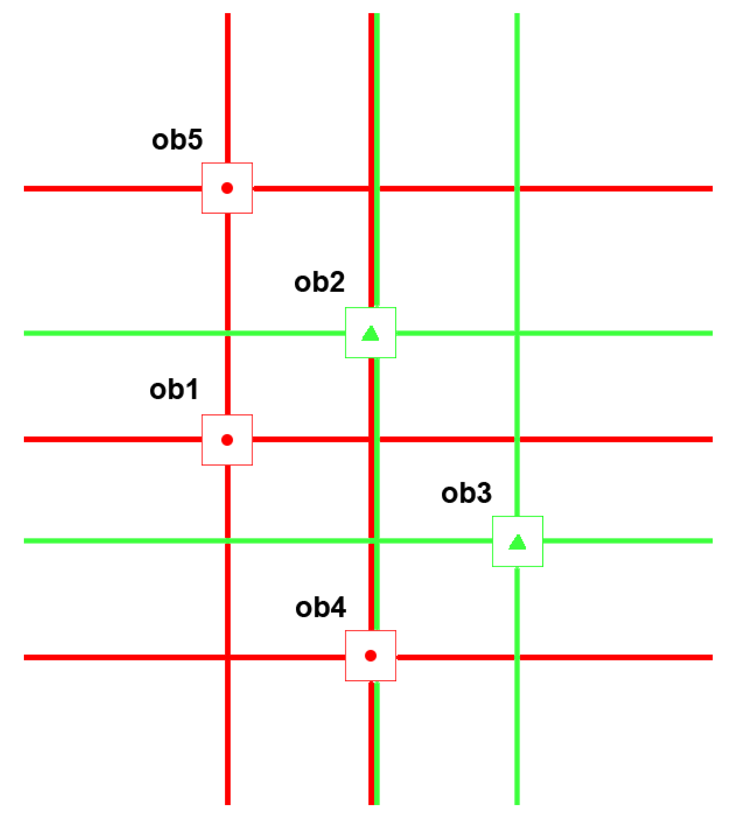
Exemplary visualization of granulation process is presented in Figure 1.

4. Epsilon Variant of Homogenous Granulation

The only difference according to homogenous granulation described in Section 3.1 is the addition of the parameter $\epsilon$, which allows us to use a floating point value in the process of granulation. The rest of the techniques are similar.

The method is defined in the following way,

$$g_{r_u}^{\epsilon ,homogenous}=\{v\in U:|g_{r_u}^{\epsilon -cd}|-|g_{r_u}^{\epsilon }|=0,forminimal{r}_{u}fulfillstheequation\}$$

(8)

where

$$g_{r_u}^{\epsilon ,cd}\left(u\right)=\{v\in U:\frac{IN{D}_{\epsilon }(u,v)}{\left|A\right|}\le r_{u}ANDd\left(u\right)=d\left(v\right)\}$$

and

$$g_{r_u}^{\epsilon }\left(u\right)=\{v\in U:\frac{IN{D}_{\epsilon }(u,v)}{\left|A\right|}\le r_u\}$$

$$r_u=\{\frac{0}{\left|A\right|},\frac{1}{\left|A\right|},\dots ,\frac{\left|A\right|}{\left|A\right|}\}$$

$$IN{D}_{\epsilon }(u,v)=\{a\in A:\frac{\left|a\right(u)-a(v\left)\right|}{ma{x}_a-mi{n}_a}\le \epsilon \}$$

where $ma{x}_a$, $mi{n}_a$ are the maximal and minimal attribute values for $a\in A$ in the original dataset.

The metrics for epsilon granulation and classification are defined in Equations (9) and (10) respectively. The Hamming metric for symbolic data is placed in Equation (9). $\epsilon$-normalized Hamming metric as modification for numerical values, for given $\epsilon$ is in Equation (10).

$$d_H(u,v)=|\{a\in A:a\left(u\right)\ne a\left(v\right)\}|.$$

(9)

$$d_{H,\epsilon }(u,v)=|\{a\in A:\frac{|a(u)-a(v)|}{ma{x}_a-mi{n}_a}>\epsilon \}|.$$

(10)

Considering training decision system from

Table 3. Training data system $(U_{trn},A,d)$, (a sample from australian credit dataset), for $\epsilon =0.05$.

	${\mathit{b}}_1$	${\mathit{b}}_2$	${\mathit{b}}_3$	${\mathit{b}}_4$	${\mathit{b}}_5$	${\mathit{b}}_6$	${\mathit{b}}_7$	${\mathit{b}}_8$	${\mathit{b}}_9$	${\mathit{b}}_{10}$	${\mathit{b}}_{11}$	${\mathit{b}}_{12}$	${\mathit{b}}_{13}$	d
$u_1$	1	$20.17$	$8.17$	2	6	4	$1.96$	1	1	14	0	2	60	159	1
$u_2$	1	$34.92$	5	2	14	8	$7.5$	1	1	6	1	2	0	1001	1
$u_3$	1	$58.58$	$2.71$	2	8	4	$2.415$	0	0	0	1	2	320	1	0
$u_4$	1	$29.58$	$4.5$	2	9	4	$7.5$	1	1	2	1	2	330	1	1
$u_5$	0	$19.17$	$0.58$	1	6	4	$0.585$	1	0	0	1	2	160	1	0
$u_6$	1	$23.08$	$2.5$	2	8	4	$1.085$	1	1	11	1	2	60	2185	1
$u_7$	0	$21.67$	$11.5$	1	5	3	0	1	1	11	1	2	0	1	1
$u_8$	1	$27.83$	1	1	2	8	3	0	0	0	0	2	176	538	0
$u_9$	1	$41.17$	$1.33$	2	2	4	$0.165$	0	0	0	0	2	168	1	0
$u_{10}$	1	$41.58$	$1.75$	2	4	4	$0.21$	1	0	0	0	2	160	1	0
$u_{11}$	1	$22.5$	$0.12$	1	4	4	$0.125$	0	0	0	0	2	200	71	0
$u_{12}$	1	$33.17$	$3.04$	1	8	8	$2.04$	1	1	1	1	2	180	18028	1
$u_{13}$	$1.234$	$22.08$	$11.46$	2	4	4	$1.585$	0	0	0	1	2	100	1213	0
$u_{14}$	0	$58.67$	$4.46$	2	11	8	$3.04$	1	1	6	0	2	43	561	1
$u_{15}$	1	$33.5$	$1.75$	2	14	8	$4.5$	1	1	4	1	2	253	858	1
$u_{16}$	0	$18.92$	9	2	6	4	$0.75$	1	1	2	0	2	88	592	1
$u_{17}$	1	20	$1.25$	1	4	4	$0.125$	0	0	0	0	2	140	5	0
$u_{18}$	1	$19.5$	$9.58$	2	6	4	$0.79$	0	0	0	0	2	80	351	0
$u_{19}$	0	$22.67$	$3.8$	2	8	4	$0.165$	0	0	0	0	2	160	1	0
$u_{20}$	1	$17.42$	$6.5$	2	3	4	$0.125$	0	0	0	0	2	60	101	0
$u_{21}$	1	$41.42$	5	2	11	8	5	1	1	6	1	2	470	1	1
$u_{22}$	1	$20.67$	$1.25$	1	8	8	$1.375$	1	1	3	1	2	140	211	0
$u_{23}$	1	$48.08$	$6.04$	2	4	4	$0.04$	0	0	0	0	2	0	2691	1
$u_{24}$	0	$28.17$	$0.58$	2	6	4	$0.04$	0	0	0	0	2	260	1005	0

the hand example of $\epsilon$ homogenous granulation is as follows.

The granules are computed below:

• $g_{0.571429}\left(u_1\right)=\left(u_1\right),$
• $g_{0.5}\left(u_2\right)=(u_2,u_4,u_{15},u_{21}),$
• $g_{0.571429}\left(u_3\right)=(u_3,u_9,u_{19},u_{20}),$
• $g_{0.5}\left(u_4\right)=(u_1,u_2,u_4,u_6,u_{21}),$
• $g_{0.5}\left(u_5\right)=(u_5,u_{10},u_{19},u_{24}),$
• $g_{0.5}\left(u_6\right)=(u_1,u_4,u_6),$
• $g_{0.5}\left(u_7\right)=\left(u_7\right),$
• $g_{0.5}\left(u_8\right)=(u_8,u_9,u_{11},u_{17}),$
• $g_{0.642857}\left(u_9\right)=(u_9,u_{10},u_{11},u_{17},u_{19},u_{20}),$
• $g_{0.642857}\left(u_{10}\right)=(u_9,u_{10},u_{19}),$
• $g_{0.642857}\left(u_{11}\right)=(u_9,u_{11},u_{17},u_{19},u_{20}),$
• $g_{0.642857}\left(u_{12}\right)=\left(u_{12}\right),$
• $g_{0.571429}\left(u_{13}\right)=\left(u_{13}\right),$
• $g_{0.428571}\left(u_{14}\right)=(u_2,u_{14},u_{16},u_{21}),$
• $g_{0.5}\left(u_{15}\right)=(u_2,u_{12},u_{15},u_{21}),$
• $g_{0.5}\left(u_{16}\right)=(u_1,u_{14},u_{16}),$
• $g_{0.642857}\left(u_{17}\right)=(u_9,u_{11},u_{17},u_{20}),$
• $g_{0.642857}\left(u_{18}\right)=\left(u_{18}\right),$
• $g_{0.571429}\left(u_{19}\right)=(u_3,u_9,u_{10},u_{11},u_{17},u_{19},u_{20},u_{24}),$
• $g_{0.642857}\left(u_{20}\right)=(u_9,u_{11},u_{17},u_{19},u_{20}),$
• $g_{0.5}\left(u_{21}\right)=(u_2,u_4,u_{14},u_{15},u_{21}),$
• $g_{0.642857}\left(u_{22}\right)=\left(u_{22}\right),$
• $g_{0.642857}\left(u_{23}\right)=\left(u_{23}\right),$
• $g_{0.642857}\left(u_{24}\right)=\left(u_{24}\right),$

Granules covering training system by random choice:

• Covering granules: $g_{0.5}\left(u_2\right)=(u_2,u_4,u_{15},u_{21}),$
• $g_{0.571429}\left(u_3\right)=(u_3,u_9,u_{19},u_{20}),$
• $g_{0.5}\left(u_5\right)=(u_5,u_{10},u_{19},u_{24}),$
• $g_{0.5}\left(u_6\right)=(u_1,u_4,u_6),$
• $g_{0.5}\left(u_7\right)=\left(u_7\right),$
• $g_{0.5}\left(u_8\right)=(u_8,u_9,u_{11},u_{17}),$
• $g_{0.642857}\left(u_{12}\right)=\left(u_{12}\right),$
• $g_{0.571429}\left(u_{13}\right)=\left(u_{13}\right),$
• $g_{0.5}\left(u_{16}\right)=(u_1,u_{14},u_{16}),$
• $g_{0.642857}\left(u_{18}\right)=\left(u_{18}\right),$
• $g_{0.642857}\left(u_{20}\right)=(u_9,u_{11},u_{17},u_{19},u_{20}),$
• $g_{0.5}\left(u_{21}\right)=(u_2,u_4,u_{14},u_{15},u_{21}),$
• $g_{0.642857}\left(u_{22}\right)=\left(u_{22}\right),$
• $g_{0.642857}\left(u_{23}\right)=\left(u_{23}\right),$

Final approximation of training decision system is in

Table 4. Granular decision system formed from Covering granules.

	${\mathit{b}}_1$	${\mathit{b}}_2$	${\mathit{b}}_3$	${\mathit{b}}_4$	${\mathit{b}}_5$	${\mathit{b}}_6$	${\mathit{b}}_7$	${\mathit{b}}_8$	${\mathit{b}}_9$	${\mathit{b}}_{10}$	${\mathit{b}}_{11}$	${\mathit{b}}_{12}$	${\mathit{b}}_{13}$	d
$g_{0.5}\left(u_2\right)$	1	$34.92$	5	2	14	8	$7.5$	1	1	6	1	2	0	1001	1
$g_{0.571429}\left(u_3\right)$	1	$58.58$	$2.71$	2	8	4	$0.165$	0	0	0	0	2	320	1	0
$g_{0.5}\left(u_5\right)$	0	$19.17$	$0.58$	2	6	4	$0.21$	1	0	0	0	2	160	1	0
$g_{0.5}\left(u_6\right)$	1	$20.17$	$8.17$	2	6	4	$1.96$	1	1	14	1	2	60	159	1
$g_{0.5}\left(u_7\right)$	0	$21.67$	$11.5$	1	5	3	0	1	1	11	1	2	0	1	1
$g_{0.5}\left(u_8\right)$	1	$27.83$	$1.33$	1	2	4	$0.165$	0	0	0	0	2	176	1	0
$g_{0.642857}\left(u_{12}\right)$	1	$33.17$	$3.04$	1	8	8	$2.04$	1	1	1	1	2	180	18,028	1
$g_{0.571429}\left(u_{13}\right)$	$1.234$	$22.08$	$11.46$	2	4	4	$1.585$	0	0	0	1	2	100	1213	0
$g_{0.5}\left(u_{16}\right)$	0	$20.17$	$8.17$	2	6	4	$1.96$	1	1	14	0	2	60	561	1
$g_{0.642857}\left(u_{18}\right)$	1	$19.5$	$9.58$	2	6	4	$0.79$	0	0	0	0	2	80	351	0
$g_{0.642857}\left(u_{20}\right)$	1	$22.5$	$1.33$	2	4	4	$0.165$	0	0	0	0	2	168	1	0
$g_{0.5}\left(u_{21}\right)$	1	$34.92$	5	2	14	8	$7.5$	1	1	6	1	2	0	1001	1
$g_{0.642857}\left(u_{22}\right)$	1	$20.67$	$1.25$	1	8	8	$1.375$	1	1	3	1	2	140	211	0
$g_{0.642857}\left(u_{23}\right)$	1	$48.08$	$6.04$	2	4	4	$0.04$	0	0	0	0	2	0	2691	1

:

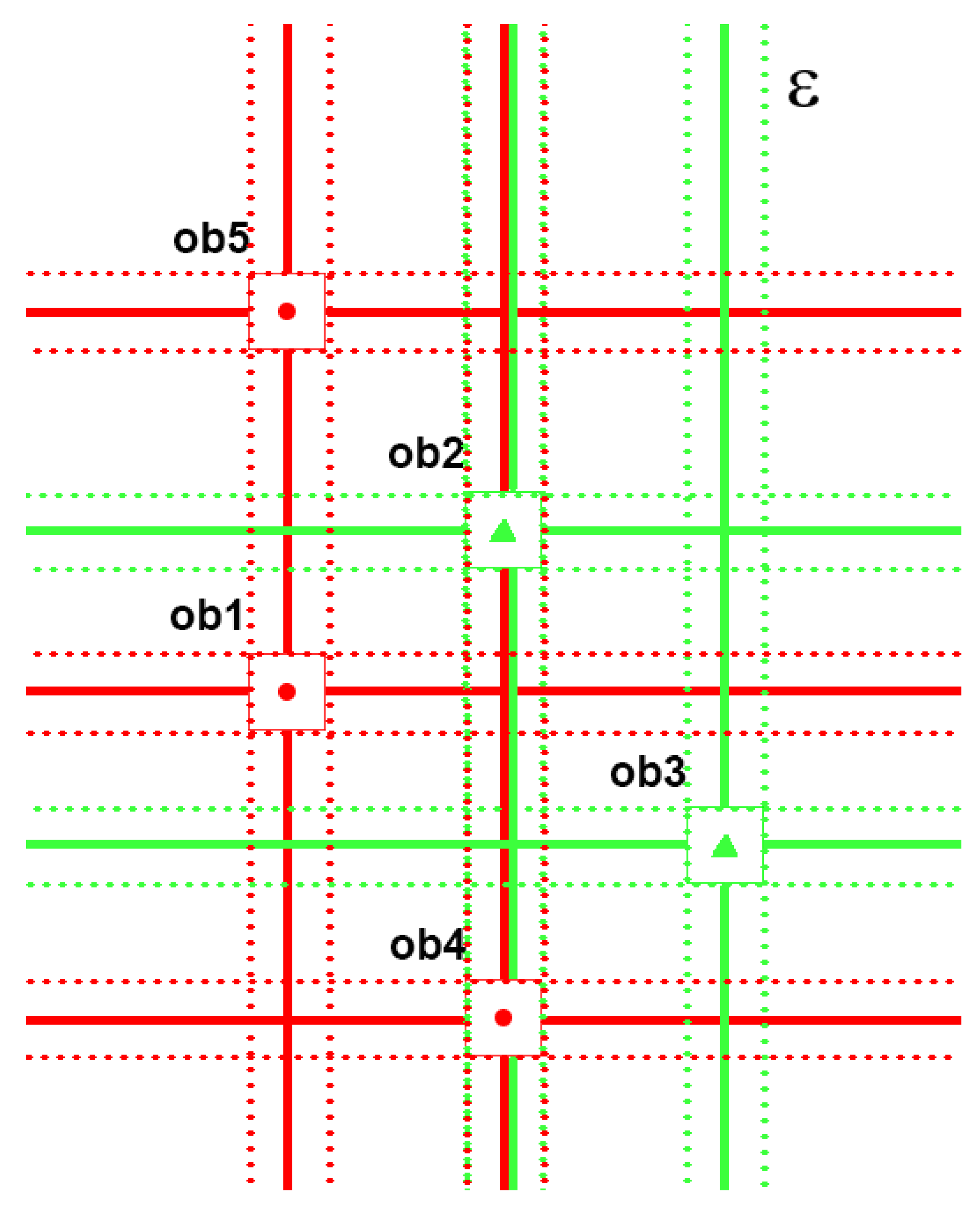
In the Figure 2 there is a simple visualization of granulation process.

5. Description of Classifier Used for Evaluation of the Granulation

A $kNN$ classifier has been used in the experiments to verify the effectiveness of approximation. The procedure is as follows.

Step 1.

The training granular decision system $(G_{r_{gran}}^{trn},A,d)$ and the test decision system $(U_{tst},A,d)$ are given, where A is a set of conditional attributes, d is the decision attribute, and $r_{gran}$ a granulation radius.

Step 2.

Classification of test objects, by means of granules of training objects, is performed as follows.

For all conditional attributes $a\in A$, training objects $v\in G^{trn}$, and test objects $u\in U_{tst}$, we compute weights $w(u,v)$ based on the Hamming metric.

In the voting procedure of the $kNN$ classifier, we use optimal k estimated by CV5, details of the procedure are highlighted in the next section.

If the cardinality of the smallest training decision class is less than k, we apply the value for $k=\left|thesmallesttrainingdecisionclass\right|.$

The test object u is classified by means of weights computed for all training objects v. Weights are sorted in ascending order as,

$$w_1^{c_1}(u,v_1^{c_1})\le w_2^{c_1}(u,v_2^{c_1})\le \dots \le w_{|C_1|}^{c_1}(u,v_{|C_1|}^{c_1});$$

$$w_1^{c_2}(u,v_1^{c_2})\le w_2^{c_2}(u,v_2^{c_2})\le \dots \le w_{|C_2|}^{c_2}(u,v_{|C_2|}^{c_2});$$

$$\dots$$

$$w_1^{c_m}(u,v_1^{c_m})\le w_2^{c_m}(u,v_2^{c_m})\le \dots \le w_{|C_m|}^{c_m}(u,v_{|C_m|}^{c_m}),$$

where $C_1,C_2,\dots ,C_m$ are all decision classes in the training set.

Based on computed and sorted weights, training decision classes vote by means of the following parameter, where c runs over decision classes in the training set,

$$Concept\_weigh{t}_c\left(u\right)=\sum _{i=1}^k{w}_i^c(u,v_i^c).$$

(11)

Finally, the test object u is classified into the class c with a minimal value of $Concept\_weigh{t}_c\left(u\right)$.

After all test objects u are classified, the quality parameter of accuracy (acc) is computed, according to the formula

$$acc=\frac{numberofcorrectlyclassifiedobjects}{numberofclassifiedobjects}.$$

(12)

Parameter Estimation in $kNN$ Classifier

In our experiments, we use the classical version of $kNN$ classifier based on the Hamming metric. In the first step, we estimate the optimal k based on 5× CV5 cross-validation on the part of dataset. In the next step, we use the estimated value of k in order to find k nearest objects for each decision class and then voting is performed to select the decision. If the value of k is larger than the smallest training decision class cardinality then k value is equal to cardinality of this class.

In

Table 5. Estimated parameters for $kNN$ based on $5\times CV5$ cross–validation, data from UCI Repository [20].

$\mathit{Name}$	$\mathit{Optimal}\mathit{k}$
$Australian$-$credit$	5
$CarEvaluation$	8
$Diabetes$	3
$German$-$credit$	18
$Heartdisease$	19
$Hepatitis$	3
$Nursery$	4
$SPECTFHeart$	14

we can see the estimated values of k for all tested datasets. These values were chosen as optimal based on the experiments with various values of k and results estimated by multiple $CV5$ operations.

6. The Results of Experiments

To show the effectiveness of the new method, we have carried out a series of experiments with real data from University of Irvine Repository (see [20]). The reference classifier is $kNN$ with Cross Validation 5 model. Data for experiments are listed in

Table 6. Basic information about datasets-[20].

$\mathit{Name}$	$\mathit{Attr}\mathit{Type}$	$\mathit{Attr}\mathit{no}.$	$\mathit{Obj}\mathit{no}.$	$\mathit{Class}\mathit{no}.$
Australian-credit	$categorical,integer,real$	15	690	2
$CarEvaluation$	$categorical$	7	1728	4
$Diabetes$	$categorical,integer$	9	768	2
German-credit	$categorical,integer$	21	1000	2
$Heartdisease$	$categorical,real$	14	270	2
$Hepatitis$	$categorical,integer,real$	20	155	2
$Nursery$	$categorical$	9	12,960	5
$SPECTFHeart$	$integer$	45	267	2

. The k parameter was evaluated in our previous works [14]. The list of optimal parameters of k is shown in Table 5. The single test consists of splitting the data into training and test set, where the training samples are granulated using our homogenous method. The results of the experiments are presented in

Table 7. The result for dynamic granulation; $5\times CV5$ method with $kNN$ classifier; $acc\_5CV5=averageaccuracy$, $GS\_size=granulardecisionsystemsize$, $TRN\_size=trainingsetsize$, $TRN\_reduction=reductioninobjectnumberintrainingsize$, $radii\_range=spectrumofradii$.

$\mathit{Name}$	$\mathit{acc}$	$\mathit{GS}\_\mathit{size}$	$\mathit{TRN}\_\mathit{size}$	$\mathit{TRN}\_\mathit{reduction}$	$\mathit{radii}\_\mathit{range}$
Australian-credit	$0.835$	$286.52$	552	$48.1\%$	$r_u\ge 0.5$
$CarEvaluation$	$0.797$	$728.5$	1382	$47.3\%$	$r_u\ge 0.667$
$Diabetes$	$0.653$	$488.9$	614	$20.4\%$	$r_u\ge 0.25$
German-credit	$0.725$	$513.3$	800	$35.8\%$	$r_u\ge 0.6$
$Heartdisease$	$0.833$	$120.5$	216	$44.2\%$	$r_u\ge 0.461$
$Hepatitis$	$0.88$	$46.16$	124	$62.8\%$	$r_u\ge 0.579$
$Nursery$	$0.607$	$9009.1$	10368	$13.1\%$	$r_u\ge 0.875$
$SPECTFHeart$	$0.763$	$138.75$	214	$35.2\%$	$r_u\ge 0.068$

. We have shown the comparable effectiveness of this new method in comparison with our best concept dependent granulation method; see

Table 8. Summary of results for $kNN$ Classifier, granular and non granular case, $acc$ = accuracy of classification, $red$ = percentage reduction in object number, r = granulation radius, $method$ = variant of Naive Bayes classifier, $nil.acc$ = non granular case.

$\mathit{Name}$	$\mathit{acc},\mathit{red},\mathit{r}$	$\mathit{nil}.\mathit{acc}$
$Australian$-$credit$	$0.851,71.86,0.571$	$0.855$
$CarEvaluation$	$0.865,73.23,0.833$	$0.944$
$Diabetes$	$0.616,74.74,0.25$	$0.631$
$German$-$credit$	$0.724,59.85,0.65$	$0.73$
$Heartdisease$	$0.83,67.69,0.538$	$0.837$
$Hepatitis$	$0.884,60,0.632$	$0.89$
$Nursery$	$0.696,77.09,0.875$	$0.578$
$SPECTFHeart$	$0.802,60.3,0.114$	$0.779$

. The new technique is significantly different from existing methods. Dynamic tuning of radius during granulation results with granules directed on decisions of their central objects. The radius is selected in automatic way during granulation process so there is no need to estimate optimal radius of granulation. The approximation level depends on objects indiscernibility ratio in the particular decision classes. Epsilon variant; see

Table 9. The result for homogenous granulation ($HG$) and for epsilon homogenous granulation ($\epsilon -HGS$); $5\times CV5$; $HG\_acc=$ average accuracy for $HG$, $\epsilon -HG\_acc$ average accuracy for $\epsilon -HGS$, $HGS\_size=$$HG$ decision system size, $\epsilon -HGS\_size=$$\epsilon -HGS$ decision system size, $TRN\_size=trainingsetsize$, $H{G}_{T}RN\_red=$ reduction in object number in training set for $HG$, $\epsilon -HGS\_size=$ reduction in object number in training set for $\epsilon -HGS$, $HG\_r\_range=$ spectrum of radii for $HG$, $\epsilon -HG\_r\_range=$ spectrum of radii for $\epsilon -HGS$, $dat{a}_1$ = Australian-credit, $dat{a}_2$ = German-credit, $dat{a}_3$ = Heartdisease, $dat{a}_4$ = Hepatitis.

	${\mathit{Data}}_1$	${\mathit{Data}}_2$	${\mathit{Data}}_3$	${\mathit{Data}}_4$
$HG\_acc$	$0.835$	$0.725$	$0.833$	$0.88$
$\epsilon -HG\_acc$	$0.842$	$0.725$	$0.831$	$0.87$
$HGS\_size$	$286.52$	$513.3$	$120.5$	$46.16$
$\epsilon -HGS\_size$	$274.52$	503	$109.4$	$46.2$
$TRN\_size$	552	800	216	124
$H{G}_{T}RN\_red$	$48.1\%$	$35.8\%$	$44.2\%$	$62.8\%$
$\epsilon H{G}_{T}RN\_red$	$50.3\%$	$37.1\%$	$49.4\%$	$62.7\%$
$HG\_r\_range$	$r_u\ge 0.5$	$r_u\ge 0.6$	$r_u\ge 0.461$	$r_u\ge 0.579$
$\epsilon -HG\_r\_range$	$r_u\ge 0.571$	$r_u\ge 0.65$	$r_u\ge 0.615$	$r_u\ge 0.579$

is fully comparable to the homogenous method and works more precisely for numerical data.

7. Conclusions

In this work, we have the results of experiments for our new granulation techniques; homogenous and epsilon homogenous granulation. The main advantage of this methods is that there is no need of parameter estimation during approximation. The parameters are tuned in an automatic way by lowering the indiscernibility ratio until the granule contains objects from the same decision class. The reduction of the size of the original decision systems is up to 50 percent. In future works, we plan to check the best classification methods for our new approximation algorithms. Additionally, we wonder if tolerating a fixed percentage of objects from other classes in the granule could improve the quality of classification.

References

- Polkowski, L. Formal granular calculi based on rough inclusions. In Proceedings of the IEEE 2005 Conference on Granular Computing GrC05, Beijing, China, 25–27 July 2005; pp. 57–62. [Google Scholar]
- Polkowski, L. A model of granular computing with applications. In Proceedings of the IEEE 2006 Conference on Granular Computing GrC06, Atlanta, GA, USA, 10–12 May 2006; pp. 9–16. [Google Scholar]
- Artiemjew, P. Classifiers from Granulated Data Sets: Concept Dependent and Layered Granulation. In Proceedings of the RSKD’07. The Workshops at ECML/PKDD’07, Warsaw, Poland, 21 September 2007; pp. 1–9. [Google Scholar]
- Artiemjew, P. A Review of the Knowledge Granulation Methods: Discrete vs. Continuous Algorithms. In Rough Sets and Intelligent Systems. ISRL 43; Skowron, A., Suraj, Z., Eds.; Springer: Berlin, Germany, 2013; pp. 41–59. [Google Scholar]
- Polkowski, L. The paradigm of granular rough computing. In Proceedings of the ICCI’07, Lake Tahoe, NV, USA, 6–8 August 2007; pp. 145–163. [Google Scholar]
- Polkowski, L. Granulation of knowledge in decision systems: The approach based on rough inclusions. The method and its applications. In Proceedings of the RSEISP 07, Warsaw, Poland, 28–30 June 2007; Lecture Notes in Artificial Intelligence. Springer: Berlin, Germany, 2007; Volume 4585, pp. 271–279. [Google Scholar]
- Polkowski, L. A unified approach to granulation of knowledge and granular computing based on rough mereology: A survey. In Handbook of Granular Computing; Pedrycz, W., Skowron, A., Kreinovich, V., Eds.; John Wiley and Sons Ltd.: Chichester, UK, 2008; pp. 375–400. [Google Scholar]
- Polkowski, L. Approximate Reasoning by Parts. An Introduction to Rough Mereology; Springer: Berlin, Germany, 2011. [Google Scholar]
- Polkowski, L.; Artiemjew, P. Granular computing: Granular classifiers and missing values. In Proceedings of the ICCI’07, Lake Tahoe, NV, USA, 6–8 August 2007; pp. 186–194. [Google Scholar]
- Polkowski, L.; Artiemjew, P. On granular rough computing with missing values. In Proceedings of the RSEISP 07, Warsaw, Poland, 28–30 June 2007; Lecture Notes in Artificial Intelligence. Springer: Berlin, Germany, 2007; Volume 4585, pp. 271–279. [Google Scholar]
- Polkowski, L.; Artiemjew, P. Towards Granular Computing: Classifiers Induced from Granular Structures. In Proceedings of the RSKD’07. The Workshops at ECML/PKDD’07, Warsaw, Poland, 21 September 2007; pp. 43–53. [Google Scholar]
- Polkowski, L.; Artiemjew, P. On granular rough computing: Factoring classifiers through granulated decision systems. In Proceedings of the RSEISP 07, Warsaw, Poland, 28–30 June 2007; Lecture Notes in Artificial Intelligence. Springer: Berlin, Germany, 2007; Volume 4585, pp. 280–290. [Google Scholar]
- Polkowski, L.; Artiemjew, P. Classifiers based on granular structures from rough inclusions. In Proceedings of the 12th International Conference on Information Processing and Management of Uncertainty in Knowledge-Based Systems IPMU’08, Torremolinos (Malaga), Spain, 22–27 June 2008; pp. 1786–1794. [Google Scholar]
- Polkowski, L.; Artiemjew, P. Granular Computing in Decision Approximation—An Application of Rough Mereology. In Intelligent Systems Reference Library 77; Springer: Berlin, Germany, 2015; pp. 1–422. ISBN 978-3-319-12879-5. [Google Scholar]
- Ropiak, K.; Artiemjew, P. On Granular Rough Computing: epsilon homogenous granulation. In Proceedings of the International Joint Conference on Rough Sets, IJCRS’18, Quy Nhon, Vietnam, 20–24 August 2018; Lecture Notes in Computer Science (LNCS). Springer: Heidelberg, Germany, 2018. [Google Scholar]
- Ropiak, K.; Artiemjew, P. A Study in Granular Computing: homogenous granulation. In Information and Software Technologies. ICIST 2018. Communications in Computer and Information Science; Dregvaite, G., Damasevicius, R., Eds.; Springer: Berlin, Germany, 2018. [Google Scholar]
- Artiemjew, P.; Ropiak, K. A Novel Ensemble Model—The Random Granular Reflections. In Proceedings of the 27th International Workshop on Concurrency, Specification and Programming, Berlin, Germany, 24–26 September 2018. [Google Scholar]
- Polkowski, L. Rough Sets. Mathematical Foundations; Physica Verlag: Heidelberg, Germany, 2002. [Google Scholar]
- Polkowski, L. A rough set paradigm for unifying rough set theory and fuzzy set theory. In Proceedings of the RSFDGrC 2003: Rough Sets, Fuzzy Sets, Data Mining, and Granular Computing, Chongqing, China, 26–29 May 2003. [Google Scholar]
- Dua, D.; Graff, C. UCI Machine Learning Repository; University of California, School of Information and Computer Science: Irvine, CA, USA, 2019; Available online: https://archive.ics.uci.edu/ml/index.php (accessed on 14 February 2019).
Figure 1.
Simple demonstration of granulation for objects represented by the pairs of attributes. In the picture we have objects of two classes, circles and triangles. Granulating the decision system in homogenous way we can obtain , , , , . The set of possible radii is .
Figure 2.
Exemplary toy demonstration for objects represented as pairs of attributes. We have two decision concepts: circles and rectangles. Epsilon homogenous granules can be , , , , . The set of possible radii is . The descriptors can be shifted in the range determined by and still were treated as indiscernible.