Learning Dispatching Rules for Scheduling: A Synergistic View Comprising Decision Trees, Tabu Search and Simulation

Abstract

A promising approach for an effective shop scheduling that synergizes the benefits of the combinatorial optimization, supervised learning and discrete-event simulation is presented. Though dispatching rules are in widely used by shop scheduling practitioners, only ordinary performance rules are known; hence, dynamic generation of dispatching rules is desired to make them more effective in changing shop conditions. Meta-heuristics are able to perform quite well and carry more knowledge of the problem domain, however at the cost of prohibitive computational effort in real-time. The primary purpose of this research lies in an offline extraction of this domain knowledge using decision trees to generate simple if-then rules that subsequently act as dispatching rules for scheduling in an online manner. We used similarity index to identify parametric and structural similarity in problem instances in order to implicitly support the learning algorithm for effective rule generation and quality index for relative ranking of the dispatching decisions. Maximum lateness is used as the scheduling objective in a job shop scheduling environment.

1. Introduction

Machine scheduling is of principal concern in the planning phase as well as the operation of manufacturing systems. It is aimed at efficiently allocating the available machines to jobs, or operations within jobs and subsequent time phasing of these jobs on individual machines [1]. Simulation procedures, analytical models and heuristics are among the traditional solution methodologies for the scheduling problem that are still widely used in industry. However, an increasing complexity of the manufacturing system necessitates a much deeper investigation of the problem domain.

Scheduling problems in the static environment have a known number of jobs and their corresponding ready times are fixed before the actual schedule execution in contrast to the dynamic environment problems in which jobs are continually revealed during the execution process [2]. Dynamic scheduling uses priority dispatching rule (PDR) to prioritize jobs waiting for processing at a resource [3]. In this approach, a score is associated dynamically for each possible assignment of a task to a particular resource. The objective is to select the task with a minimum or maximum assigned score (as the case may be) for the chosen resource [4]. Due to their ease of implementation and substantially reduced computational requirement, they remain a very popular technique despite of their poor performance in the long run [5,6].

The major drawbacks of PDRs include their performance dependence on the state of the system and non-existence of any single rule that is superior to all the others for all possible states the system might be in [7]. Meta-heuristics (e.g., simulated annealing, Tabu search, etc.) have an advantage over PDRs in terms of solution quality and robustness, however, these are usually quite difficult to implement and tune as well as computationally too complex to be used in a real-time system.

Robust and better-quality solutions provided by meta-heuristics contain useful but implicit knowledge about the problem domain and solution space explored. Such a set of solutions represents a wealth of scheduling knowledge to the domain that can be transformed in a usable form of decision tree or a rule-set. In this paper, we propose an approach to exploit this scheduling knowledge in this way. In our approach, we seek this hidden scheduling knowledge through a data mining module to identify a rule-set by exploring the patterns in the solution set obtained by an optimization module based on Tabu search, a very efficient meta-heuristic for Job-Shop Scheduling Problem (JSSP) [8,9]. This rule-set approximates the output of the optimization module when incorporated in a simulation model of the system. It is subsequently used to make dispatching decisions in an online manner.

The rest of the paper is organized as follows. First, we present a concise review of the closely related literature on the use of learning in scheduling. Subsequently, the general structure of the proposed methodology is outlined, followed by the details of each module with its working, significance and coordination with other modules. Section 3 provides a brief description of the experimental setup. The results of the experiments are then presented with a comparison to standard dispatching rules for a set of benchmark job shop scheduling problems. Finally, the paper concludes in the light of findings with a brief note on future research directions.

2. Learning in Shop Scheduling: A Concise Review

Generally, the approach of learning in shop scheduling stems from the idea of dynamic selection of the priority dispatching rules owing to the inability of traditional PDR-based job dispatching to adapt for the changing conditions of the shop floor. Extending the idea of the dynamic selection using simulation towards the dynamic modification and subsequently to the dynamic generation of new rules using the machine learning based techniques resulted in a significant increase of research interest in this area.

In the context of solving various types of shop scheduling problems, Inductive learning [10,11,12], artificial neural-networks [13], case-based reasoning [14], support vector machines [15], reinforcement learning [16], fuzzy logic [17], evolutionary learning, genetic programming [18], analytical network processes [19] and artificial immune networks [20,21] ,are among the major learning based approaches with a large number of their variants that have been employed by researchers.

Table 1. List of selected references for learning in shop scheduling.

Reference	Approach	Learning	Application
[25]	Simulation/Learning	GENREG	Simplified flow shop
[26]	Simulation/Learning	LADS	FMS with transportation
[27]	Simulation/Learning	C4.5, PDS	Flow shop with machine failure
[28]	Simulation/Learning	Inductive Learning	Flow shop, Job shop
[29]	Simulation/Learning	C4.5, BPNN, CBR	FMS with transportation
[30]	Simulation/Data Mining	C4.5	Job shop
[31]	GA/Learning	C4.5	Job shop
[32]	GA/Data Mining	Attribute Oriented Induction	Job shop
[33]	GP	C4.5	Single machine
[34]	GA/Data Mining	C4.5	Job shop
[35]	Simulation/Data Mining	C4.5	FMS
[36]	GA/Learning	C4.5	Job shop
[37]	Simulation/ Data Mining	C4.5	Single machine
[7]	GP	C4.5	Single machine, Flow shop
[38]	GA/Learning	C4.5	Job shop
[39]	GA/Learning	ANN /C4.5	FMS
[40]	Simulation/GA		Distributed manufacturing system
[41]	GP		Flexible JSSP with recirculation
[42]	Data Mining/ Timed petrinets	C4.5	Job shop
[43]	Data Mining	Preference learning	Job shop
[13]	Simulation/ Optimization	Neural networks	Flow shop

lists a few of the selected works that employed learning in scheduling. For detailed reviews on the subject, refer to [14,22,23] and an updated review by [24].

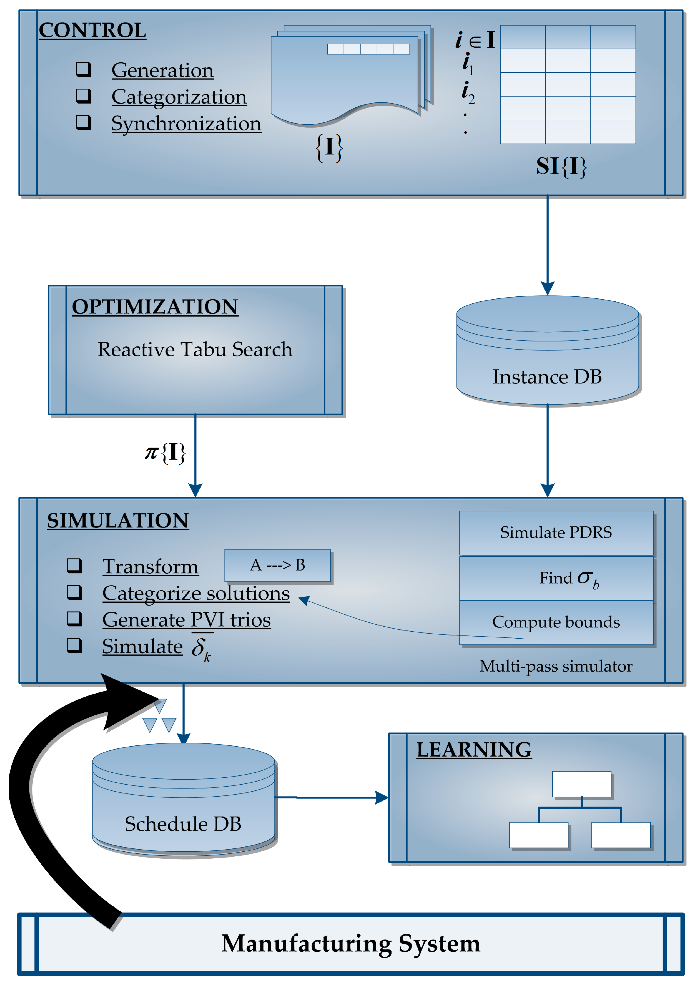
3. Proposed Methodology

The framework we propose consists of four modules, namely the control module, simulation module, optimization module and learning module. In addition, there is a set of three databases. The objective of the proposed framework is to generate a set of rules for making dispatching decisions. Our focus is on the job shop scheduling environment. Figure 1 illustrates the workflow of the proposed approach.

Initially a set of problem instances is generated by the control module under pre-specified settings. These problem instances are categorized by the control module on the basis of similarity index (SI) in order to better reflect their individual contribution. Each problem instance tagged with a vector of similarity indices is subsequently stored in an instance database.

The optimization module generates solutions in the form of sequence (π) for a subset of these instances to start with. The collection of these job shop instances and the corresponding solutions form the basis for the initial training dataset. In effect, it is an implicit collection of good scheduling decisions made by the optimization module. It is required to explicitly identify each decision and assign an index of quality to it. However, the downstream decisions significantly affect the computed index of quality. A more relevant quality index (${\tau }^{{\delta }_k}$) is obtained by taking this factor into account as well as the processing times of the operations involved in the dispatching decision. The simulation module generates and associates this quality index to each decision taken by the optimization module.

The entire collection of decisions along with the assigned quality indices are used as relevant scheduling knowledge. This scheduling knowledge is kept in a scheduling database in the form of Predictor-Value-Index (PVI) trio to be used subsequently by a learning process. As the characteristics of each solution instance are implicitly linked with the complexity and the structure of the problem, the matrix of similarity index is also used in the learning process. Based on this scheduling knowledge, a decision tree is generated by the learning process.

This decision tree is then used to dispatch the jobs-awaiting service in an online manner. The decision tree is dynamically updated, whenever necessary through a control module. The control module transmits the knowledge of good scheduling decisions to the optimization module as well to improve its own performance at subsequent levels. In the following subsections, the structure and working of each module is described in detail.

3.1. Control Module

The functions of the control module include the generation of the relevant scheduling problem instances, classification of these problem instances based upon the similarity and relative complexity and synchronization of the scheduling decisions with all the three databases.

The generation of the problem instances is a quite simple process. It includes the controlled random processes for generating a set of operations with positive processing times, assignment of these operations to the jobs and assigning a due-date to each job. The problem instances are in fact acyclic graphs with directed and undirected arcs. This is disjunctive graph representation proposed by [44] that is able to effectively represent a Job Shop Scheduling Problem (JSSP). An example of a disjunctive graph representation of a small size JSSP with four machines and three jobs is shown in Figure 2. The three jobs have ready times $r_1$, $r_2$ and $r_3$, respectively. The node ${\mathcal{O}}_{ik}$ represents operation of the $i^{\text{th}}$ job to be processed on machine $k$ with a processing time of $p_{ik}$ (labeled on edges or conjunctive arcs). The first and the last nodes are the dummy nodes. Operations to be performed on the same machine are connected through disjunctive arcs (dotted edges with arrows on both sides).

The control module creates a matrix of similarity index values for such disjunctive graphs for all problem instances. The similarity index value is an estimate of how much resemblance a problem instance has, to any other problem instance. Rajendran et al. [45] provide a survey on the various methods used in finding graph similarity. In our experiments, the computation of the similarity indices are made on the loopy belief propagation based algorithm proposed by [46]. For this purpose, it takes into account the structure of the sub-graphs over the entire set of nodes and normalized Euclidean distance among these sub-graphs.

3.2. Optimization Module

The optimization module has a pivotal role in the proposed methodology. As the learning algorithm relies on the quality of the scheduling decisions taken by the optimization module, it is very important that the solutions provided by the optimization module are of good quality. Moreover, it is desired that there is some means of quantifying the quality of these solutions. The working of the optimization modules is based on the Tabu search (TS) algorithm proposed by [47]. Jain et al. [9] found the Tabu search (TS) algorithms, in general, to be very effective for finding solutions of JSSP. This is mainly attributed to its powerful memory function [48] in coordination with neighborhood structures and flexible move evaluation strategies [5]. This is in disparity with what limited capability PDRs can do due to their myopic nature.

The optimization module finds the solutions to a selected set of problem instances that are initially referred to as efficient solutions in this methodology. This is due to the assumption that these solutions are obtained through rigorous and intelligent moves made by the algorithm. The optimization module works in an offline manner, however, it continuously provides more and more solutions to the problem instances generated by the control module.

3.3. Simulation Module

Simulation module is a multi-purpose module that is tightly integrated with all other modules. One of the key functions of the simulation module is to transform the solution provided by the optimization module into a set of dispatching decisions. Each such decision is simply a yes/no-value for a job A to be dispatched before some other job B. At each instant, when a decision is to be taken for the next job to be dispatched, all the jobs competing for a particular resource are alternatively tested (the alternate decision) as per the sequencing order provided by the optimization module.

Simulation module is also in charge for the generation of values for a set of pre-selected attributes, referred as predictors to be used by the learning module. This is done corresponding to each instant at which a dispatching decision is made. It is worth-mentioning that these decision-points (the time instants when the decision is made) are dependent on the solution provided by the optimization module as well as the problem structure and parameters. This means that for two solutions of the same quality with different sequencing order, one may have the same or different decisions points and hence the values for the selected attributes accordingly. Despite this fact, a particular decision may be same for both solutions. This is illustrated by an example of 3 × 3 problem instance given in

Table 2. A 3 × 3 problem instance.

	${\mathbf{ℳ}}_{\mathbf{1}},{\mathit{p}}_{\mathit{j}\left(\mathbf{1}\right)}$	${\mathbf{ℳ}}_{\mathbf{2}},{\mathit{p}}_{\mathit{j}\left(\mathbf{2}\right)}$	${\mathbf{ℳ}}_{\mathbf{3}},{\mathit{p}}_{\mathit{j}\left(\mathbf{3}\right)}$
${\mathcal{J}}_1$	1,2	2,6	3,4
${\mathcal{J}}_2$	1,5	2,3	3,5
${\mathcal{J}}_3$	1,3	2,1	3,3

. The schedules illustrated in Figure 3 and Figure 4 have only a difference in sequencing order at machine 2, i.e., job 3 and job 2 have interchanged their order. This does not change the $C_{\text{max}}$.

The simulation module assigns a quality index (QI) for each solution, generated by the optimization module, based on the bound that is also computed by the simulation module using multi-pass simulator. It is computed as $\text{QI}=\frac{f^{*}}{\widehat{f}}$, where $f^{*}$ and $\widehat{f}$ are respectively the values of the objective function computed by the optimization module using Tabu search and the simulation module using the best dispatching rule. This quality index is used to categorize the generated solutions for subsequent use by the learning algorithm. Each solution is included in the learning set based upon certain characteristics it possesses. These characteristics are the implicit relations among operations that govern the particular sequencing order we have for an efficient solution. It is not a trivial task to unfold these relations, however a certain set of guidelines can be attained.

The multi-pass simulator incorporated in simulation module simulates the problem instances solved by the optimization module and finds a set of schedules using a pre-defined set of PDRs. A schedule ${\sigma }_b$ with best objective value is used as a reference schedule among this set of schedules. The objective value is set as a bound, f_b or $\widehat{f}$ on the solution-set for that problem instance. This bound may be used as a characteristic for the set of the dispatching decisions, {${\delta }_k$} taken in the schedule ${\sigma }^{*}$, generated by the optimization module.

By generating an alternative dispatching decision, ${\overline{\delta }}_k$—that is, by swapping the sequence of two jobs namely $i$ and $j$ with processing times $p_i$ and $p_j$, respectively, on a machine $h$ in the schedule ${\sigma }^{*}$, the simulation module computes and assigns a quality index ${\tau }^{{\delta }_k}$ to each dispatching decision ${\delta }_k$. This is done by generating a set of active schedules, namely $\{{\sigma }_{A_k}^{*}\}$. Hence, we have as many alternate schedules as there are original dispatching decisions, $z$ made in the optimal schedule. It is worth mentioning that the computed quality index is dependent on the downstream operations. The value of the quality index, ${\tau }^{{\delta }_k}$ for a kth dispatching decision ${\delta }_k$ is computed as,

$${\tau }^{{\delta }_k}=\left[{\omega }_1\left(1-\frac{k}{z+1}\right)+{\omega }_2 \left(\frac{p_i+p_j}{p}\right)\right]\frac{f\left({\sigma }^{*},\phi \right)}{f\left({\sigma }^{*},{\overline{\delta }}_k\right)}$$

(1)

where $f\left({\sigma }^{*},{\overline{\delta }}_k\right)$ represents the value of the performance measure obtained by incorporating the dispatching decision ${\overline{\delta }}_k$ in the original schedule ${\sigma }^{*}$, and ${\omega }_1$ and ${\omega }_2$ are the weighting factors and $p$ is the remaining processing times for the jobs including $p_i$ and $p_j$. Note that $f\left({\sigma }^{*},\phi \right)$ represents the value of the performance measure for original schedule ${\sigma }^{*}$ without incorporating any change (in short, also represented as $f\left({\sigma }^{*}\right)$ or $f^{*}$). This notation is used for the consistency. It is worth-mentiong here that this quality index, ${\tau }^{{\delta }_k}$ is different from the quality index (QI), associated with the schedule. Each dispatching decision ${\delta }_k$ has its own quality index ${\tau }^{{\delta }_k}$ in contrast to the value of the lower bound, f_b, which is same for all dispatching decisions. For example, for the schedule shown in Figure 5 for a problem instance ($6 \times 6$) of

Table 3. A 6 × 6 problem instance with due dates.

$\mathcal{J}$	${\mathbf{ℳ}}_{\mathbf{i}},{\mathit{p}}_{\mathit{i}}$						${\mathit{d}}_{\mathit{i}}$
${\mathcal{J}}_1$	3,4	1,6	2,8	4,5	6,8	5,7	22
${\mathcal{J}}_2$	6,4	2,1	1,10	3,1	4,2	5,3	26
${\mathcal{J}}_3$	1,1	2,4	4,2	6,2	3,1	5,1	25
${\mathcal{J}}_4$	1,6	2,3	4,9	3,8	5,9	6,8	23
${\mathcal{J}}_5$	5,3	2,4	6,6	1,7	3,7	4,3	18
${\mathcal{J}}_6$	1,4	2,1	4,2	3,10	5,4	6,5	28

, if the sequence of operations for job 4 and job 3 on machine 2 is swapped to get a new active schedule as shown in Figure 6, we can assign a quality index ${\tau }^{{\delta }_5}$ to the dispatching decision ${\delta }_5$ (i.e., job 3 to be processed before job 4 on machine 2) as follows:

$${\tau }^{{\delta }_5}=\left[{\omega }_1\left(1-\frac{5}{20}\right)+{\omega }_2 \left(\frac{3+4}{10+37}\right)\right]\frac{24}{29}$$

(2)

where $\left({\sigma }^{*},\phi \right)=L_{max}\left({\sigma }^{*}\right)=24$, $f\left({\sigma }^{*},{\overline{\delta }}_k\right)=L_{max}\left({\sigma }^{*},{\overline{\delta }}_k\right)=29$, $k=5$ and $z=20.$

3.4. Learning Module

Learning module uses the induction process of decision trees as a learning mechanism. The conceptual process of classification of dispatching decisions stored in the schedule database is relatively simple when represented as a decision tree. This simplicity and the transparency is the major motivation in adopting the decision tree based learning for the proposed approach. In addition, decision tree based learning helps to bridge the gap between the pure reactive nature of PDR and the predictive centralized approaches that are generally prohibitive in online scheduling due to delayed response [49]. Learning module uses C4.5 algorithm for mining the implicit information in the dispatching decisions.

The dispatching decisions made by the optimization module and transformed by the simulation module are stored in a schedule database for a subsequent learning process. It is worth mentioning that all the decisions including the alternate decisions generated by the simulation module are in the same database along with the corresponding quality index. It is assumed to have a better learning accuracy even with decisions that are not generated by the optimization module. This is because we have a quality index with each decision that helps identifying the areas of greater significance in the search space.

Construction of a relevant training dataset is very crucial point in the entire KDD process. Scheduling database in the form of Predictor-Value-Index (PVI) trios form the basis for the training dataset. This information forms a number of cluster-sets for each attribute based on their values. From the data mining perspective in JSSP, the target concept to be learned is to determine which job should be dispatched first within a set of jobs that are ready to be scheduled on the same machine at a particular instant. Extracting this knowledge from the training dataset would allow us to dispatch the next job at any given time and thereafter to create dispatching lists for any set of jobs $\left[x_k y_k\right]$ forms a collection of positive training examples from a single problem instance with $k$ dispatching decisions, where $x_k=\left[x_{1k} x_{2k}\dots x_{lk}\right]$ represnts values for the $l$ selected predictors (

Table 4. Selected Predictors.

Expression	Description
$n_t$	Number of jobs in the system at any instant$t$.
$p_{max}-\overline{\vartheta }$	Difference between maximum and average remaining processing times.
$\frac{n_p}{n_t}$	Percentage of jobs with relatively longer processing times.
$\frac{n_d}{n_t}$	Percentage of jobs with relatively loose due dates.
$\overline{\vartheta }$	Average remaining processing time.
$\overline{\phi }$	Average remaining time until due-dates.
$\frac{\overline{\phi }}{\overline{\vartheta }}$	Relative tightness ratio.
$\widehat{f}$	Bound on the value of $f$, where $f =L_{\text{max}}$.
$QI$	Quality Index of the best solution among solutions provided by PDRs, $=\frac{f^{*}}{\widehat{f}}$.

) and $y_k\in \left\{0,1\right\}$ is the value for the target concept for $k^{\text{th}}$ decision. The target concept, $y_k$ ($y_k:=precede{s}_{u,v,q}$) is a binary variable representing the processing order of two jobs $u, v$ to be processed on machine $q$, i.e., $y_k=1$ represents $u\to v$ in lexical order on machine $q$ and vice versa. For each dispatching decision, we have a set of alternate dispatching decisions as negative examples with associated quality index values. For a complete set of training instances, we have a collection of $\left[x_k y_k\right]$ as positive training examples and associated negative examples for each instance of the training set.

For example, consider the schedule shown in Figure 5. At t = 0, the jobs ${\mathcal{J}}_3$, ${\mathcal{J}}_4$ and ${\mathcal{J}}_6$ compete for the machine ${ℳ}_1$. To make a dispatching decision for the position 1 on ${ℳ}_1$ and to generate the relevant data at t = 0, three comparisons are made namely (3,1) vs. (4,1), (3,1) vs. (6,1), and (4,1) vs. (6,1), where (3,1) signifies operation number 1 of ${\mathcal{J}}_3$ and so on. Since the optimization module selected ${\mathcal{J}}_6$ before ${\mathcal{J}}_4$, as shown in Figure 5, the target concept has a value of 0. Similarly, 0 is returned for other two comparisons. At t = 5, we have again three comparisons resulting value of 0 for target concept for all of them and then at t = 10, we have four comparisons, and a comparison, for instance, (1,2) vs. (5,4) returns a value of 1 for the target concept. The corresponding values of the predictors are computed at the time the decision is made. Hence we have as many rows as positive learning examples as the number of comparisons made at various decision points at each machine as per the solution generated by the optimization module.

Finally, the decision tree induced using the learning algorithm can be applied directly to the same JSSP to validate the explored knowledge and as a predictive model to predict the target concept. A set of scheduling problem instances chosen from the database in accordance with their similarity indices is to be used as a test dataset for the scheduling knowledge discovered. The overall sequence of operations obtained by these rules is translated to a schedule using a schedule generator. Thus, the tree will, given any two jobs, predict which job should be dispatched first and can be thought of as a new, previously unknown rule. In addition to the prediction, decision trees and decision rules reveal insightful structural knowledge that can be used to further enhance the scheduling decisions.

Proper selection of the relevant predictors and creation of new predictors that are more pertinent to the desired target concept has the key role in the learning process. The entire learning process significantly suffers with the poor selection and inappropriate creation of the predictors. It is the task of finding the most reasonable subset of predictors for a classifier to seek fewer predictors and maximum class separability [35]. This process is also critical for the effectiveness of the subsequent model induction by eliminating certain redundant and irrelevant predictors. Effective use of cluster-sets in tandem with selected attribute-set helps in generating a better quality decision tree.

Both the creation of new predictors and selection of predictors (we call the both process combined as attribute extraction) are primarily linked with the objectives of the JSSP. Tardiness based objectives require different predictors to be taken into account while flow-time based objectives have different requirements. For instance, deadline related statistics and counters are more suited for tardiness based objectives [50].

There exists a strong relation among the sequencing of operations due to precedence constraints, however, considering only two (operations of the) jobs to be processed by the same machine among schedulable jobs (the predecessor, if any, of whom are already dispatched) at any instance for the comparison reduces this dependency effect. Proper attribute extraction plays an important role to reduce this dependency as well.

Arithmetic combinations of primitive predictors can also be used to generate new useful predictors. However, a large set of predictors is not desirable, as the predictors are generally not independent of each other, making the process computationally impractical. Several heuristics, such as backward stepwise heuristic and forward stepwise group heuristic, have been proposed to limit the selected subset of predictors while maintaining a certain performance level [51]. Each simulation scenario as a static control rule and necessary predictors are collected at data collection points and saved in corresponding file.

4. Experimental Setup

Two sets of 6 × 6 similarly sized instances of a static job shop problem with different seed values are used as training and test data. All jobs are available simultaneously at time zero. Discrete uniform distribution between 1 and 10 is used to generate the operation processing times. The job due dates are determined using two parameters $\tau$ and $\rho$, where $\tau$ determines the expected number of tardy jobs (and hence the average tightness of the due dates) and $\rho$ specifies the due date range. Once these parameters have been specified, the job due dates are generated from the discrete uniform distribution given as,

$$d_j=U[\mu -\frac{\mu \rho }{2},\mu +\frac{\mu \rho }{2}]$$

(3)

where $\mu = \left(1 - \tau \right)E\left[C_{\text{max}} \right]$ is the mean due date. $E\left[C_{max} \right]$ denotes the expected makespan for the problem instance and is calculated as,

$$E\left[C_{\text{max}} \right]=\frac{{{\displaystyle \sum }}_{jϵ\mathcal{J}}{p}_j}{m}$$

(4)

Note that this assumes no idle time on machines, and hence will be an optimistic estimate of $C_{\text{max}}$. We consider $\tau = 0.3$ and $\rho = 0.5$ with $L_{\text{max}}$ (Maximum Lateness) used as the scheduling objective.

Table 5. Summary of parameters for experimental setup.

Parameter	Value
Datasets	Training Dataset, $I$ and Test Dataset, ($\acute{I}$)
Problem size	$6\times 6$
Number of training instances, $⋕I$	$100$
Number of test instances, $⋕\acute{I}$	$100$
Release dates, $r_j$	$0$
Operation processing times, $p_{j\left(i\right)}$	$\mathrm{U}\left[1,10\right]$
Due-dates, $d_j$	$\mathrm{U}\left[\mu -\frac{\mu \rho }{2},\mu +\frac{\mu \rho }{2}\right]$
${\omega }_1, {\omega }_2$	$0.6,0.4$
$\tau , \rho$	$0.3,0.5$
Objective function, $f$	$L_{\text{max}}$

lists the parameters used in the experimental setup.

Selection of the relevant predictors has a key role in obtaining the appropriate performance level. High dimensionality poses a challenge to learning tasks. Due to irrelevant predictors, classification algorithms tend to over-fit training data and degrade the generalization ability [52,53]. The selected predictors have the following characteristics: the predictors are related to tardiness based performance measures. It is preferred to define predictors in relative values instead of absolute values. The predictors with high variation are discretized. Table 4 lists the predictors used in the experiments. The selection of these predictors is generally on the basis of earlier research (see for example, [35,54,55]). It is acknowledged though that a simple attribute-selection model is not capable to generate and guarantee even near-optimal subset of predictors. A more rigorous approach for the combinatorial attribute selection may be used at the cost of extra computational complexity (see [56] for review and limitations of other approaches).

The predictors $p_{max}-\overline{\vartheta }$ and $\overline{\vartheta }$ use the remaining processing time for direct comparison of two jobs, as an average measure and relative value among all the jobs in system. It is important to note that it is the combined effect of these predictors along-with others, which plays a role in strengthening their relation with the target concept. For example, $\overline{\vartheta }$ in relation with $n_t$ and $p_{max}-\overline{\vartheta }$ affects the $\raisebox{1ex}{$n_p$}\!\left/ \!\raisebox{-1ex}{$n_t$}\right.$. Hence it is not a very trivial task to identify a relationship of predictor with the target concept. The bound on the value of the performance measure is also used as a predictor, however it is again not independent from the other selected predictors.

For this study, we used the binning method—an unsupervised discretization method—to establish banded categories for the predictor values. Based on the values of the mean and standard deviation of the distribution of the specified predictor(s), we generate a field with banded categories. Figure 7 illustrates a ±3 standard deviation based discretization for a predictor to generate seven bins. However, creating banded categories based on standard deviations may result in some bins being defined outside the actual data range and even outside the range of possible data values, affecting the contribution of the predictor in the learning process.

5. Results and Discussion

The decision tree with a maximum allowed limit of 30 splits along with the cross validation is grown using the experimental setup described with training dataset consisting of 100 instances. A set of 49 rules with a class labeling error of 28.06% is obtained. It is observed that there is no significant improvement in the class error by allowing more number of splits.

The rule-set is applied to the instances of the test set. Figure 8 shows the box plot of $L_{\text{max}}$ values for the set of PDRs given in

Table 6. Definitions of benchmark priority dispatching rules.

Rule	Definition	Rank	Priority index
FIFO	First in first out	min	$C_{j\left(i-1\right)}$
SI	Shortest imminent processing time	min	$p_{j\left(i\right)}$
SPT	Shortest processing time	min	$p_j$
EDD	Earliest due-date	min	$d_j$
SLACK	Slack	min	$d_j-t-{\displaystyle \sum }_{i=1}^{o_j}{p}_{j\left(i\right)}$
CR	Critical Ratio	min	$\frac{d_j-t}{{{\displaystyle \sum }}_{i=1}^{o_j}{p}_{j\left(i\right)}}$
CRSI	Critical Ratio/Shortest Imminent	min	$\frac{d_j-t}{{{\displaystyle \sum }}_{i=1}^{o_j}{p}_{j\left(i\right)}}$
MOD	Modified operation due date	min	$\max \left(d_{jk},t+p_{jk}\right)$
COVERT	Cost over time	max	$\frac{1}{p_{j\left(i\right)}}{\left(1-\frac{{\left(d_j-t-{{\displaystyle \sum }}_{i=l}^{o_j}{p}_{j\left(i\right)}\right)}^{+}}{h_1{{\displaystyle \sum }}_{i=l}^{o_j}{p}_{j\left(i\right)}}\right)}^{+}$
ATC	Apparent tardiness cost	max	$\frac{1}{p_{j\left(i\right)}}exp{\left(-\frac{\left(d_j-t-p_{j\left(i\right)}-{{\displaystyle \sum }}_{i=l+1}^{o_j}{p}_{j\left(i\right)}\right)}{h_3{{\displaystyle \sum }}_{i=l}^{o_j}{p}_{j\left(i\right)}}\right)}^{+}$
MF	Multi-factor	max	$\frac{1}{p_{j\left(i\right)}}\left(W_{j\left(i\right)}-(d_j-t-{\displaystyle \sum }_{i=l}^{o_j}{p}_{j\left(i\right)}\right)$ where $W_{j\left(i\right)}={\displaystyle \sum }_{i=k}^{n\left(\ne k\right)}{\displaystyle \sum }_{j=1}^q{p}_{j\left(i\right)}-{\displaystyle \sum }_{j=1}^{q-1}{p}_{j\left(i\right)}$
CEXSPT	Conditionally expediting SPT	-	Partition into three queues, late queue, operationally late queue and ahead-of-schedule queue, with SI as selection criterion within queues. Shifting of job to other queues is not allowed.

, Tabu search used in the optimization module and the rule-set obtained by the decision tree based learning algorithm. The validation accuracy of the rule-set obtained is found to be 60.5%. Figure 9 shows the plot of the confusion matrix for the decision tree grown.

It is worth mentioning that another grown decision tree employing the quality index, ${\tau }^{{\delta }_k}$ as an additional predictor results in a significant boost to the validation accuracy with a set of 37 rules while all other parameters remain the same. This is illustrated in Figure 10 using the confusion matrix plot of the decision tree. This requires computations for the quality index of each decision, which is an expensive process. The tree we obtained by including the quality index predictor for the test instances requires these computations a priori based on the optimal decisions made by the optimization algorithm. However, a procedure to find an estimate for the value of the quality index would result in better performance.

A comparison of the two confusion matrix plots reveals that the original decision tree was unable to effectively predict the class with label 0, i.e., the operation not selected as the first operation resulting in the specificity value to be 3.9 %. This value is significantly increased to 77.3% with the inclusion of ${\tau }^{{\delta }_k}$ in the predictor-set.

6. Conclusions

A synergy of optimization, simulation and learning is used to better address the problem of shop scheduling. The cooperative interaction of these areas is desired in scheduling due to the proven effectiveness of each of them separately. Optimization provides with efficient schedules but the computational complexity prohibits its use in an online manner. Dispatching rules are quick but lack robustness and adaptability. Simulation enables making a comparison of the effectiveness of dispatching rules, analyzing behavior of scheduling strategies and understanding the problem domain. Learning makes use of the implicit knowledge contained in the problem domain and efficient solution domain to approximate the behavior of efficient solution domain identified by the optimization.

A detailed description of the arrangement and functionality of different modules of the proposed methodology is provided. For a set of similar-size instances of job shop scheduling problem, the results on the maximum lateness using the proposed methodology are presented. In most of the real-world sized JSSPs, the optimal solutions are not obtainable or implementable due to the complex dynamic nature of the problem. However, through this approach several alternative solutions could be proposed that are not only sufficiently efficient but as easy to implement as the traditional dispatching rules are. However the underlying assumption for an effective implementation of the methodology is that the optimization process is able to capture the inherent problem structure in regards with the scheduling objectives. A natural extension of the proposed methodology in this context would be to reuse this knowledge in order to effectively solve the problem instances of matching similarity index.

By making use of alternative dispatching decisions, we associated a quality index to each dispatching decision. This value estimates the significance of a particular dispatching decision. In combination with a group of similar decisions arising from different or similar problem instances, learning algorithm is able to build a density map of the dispatching decision. This helps in analyzing the efficient schedules in comparison with relatively less efficient schedules.

One of the objectives of the proposed approach is to capture the effect of disjunctive constraints on the dispatching decision during the different phases of the schedule generation. This is partially achieved by fairly improved prediction accuracy, however it lacks the implementation scheme for the test instances. Moreover, an improved metric for the quality index may be devised for superior performance.

It is not unusual to have a different set of selected predictors in regards with scheduling objective. In fact, it is a key factor for the successful implementation of the proposed framework. Predictor selection for different objectives and their combinations has to be rigorously explored to obtain compact and efficient rule set.

References

1. Shaw, M.J.; Park, S.; Raman, N. Intelligent Scheduling with Machine Learning Capabilities: The Induction of Scheduling Knowledge. IIE Trans. 1992, 24, 156–168. [Google Scholar] [CrossRef]
2. Sidney, J.B. Sequencing and scheduling-an introduction to the mathematics of the job-shop, by Simon French, Wiley, 1982, 245 pp. Networks 1983, 13, 310–311. [Google Scholar] [CrossRef]
3. Vieira, G.E.; Herrmann, J.W.; Lin, E. Rescheduling manufacturing systems: A Framework of Strategies, Policies, and Methods. J. Sched. 2003, 6, 39–62. [Google Scholar] [CrossRef]
4. Montana, D. A comparison of combinatorial optimization and dispatch rules for online scheduling. Mag. West. Hist. 2005, 353–362. [Google Scholar]
5. Jain, A.S.; Rangaswamy, B.; Meeran, S. New and “stronger” job-shop neighbourhoods: A Focus on the Method of Nowicki and Smutnicki (1996). J. Heuristics 2000, 6, 457–480. [Google Scholar] [CrossRef]
6. Pierreval, H.; Mebarki, N. Dynamic scheduling selection of dispatching rules for manufacturing system. Int. J. Prod. Res. 1997, 35, 1575–1591. [Google Scholar] [CrossRef]
7. Geiger, C.D.; Uzsoy, R.; Aytuǧ, H. Rapid modeling and discovery of priority dispatching rules: An Autonomous Learning Approach. J. Sched. 2006, 9, 7–34. [Google Scholar] [CrossRef]
8. Zhang, C.; Li, P.; Guan, Z.; Rao, Y. A tabu search algorithm with a new neighborhood structure for the job shop scheduling problem. Comput. Oper. Res. 2007, 34, 3229–3242. [Google Scholar] [CrossRef]
9. Jain, A.S.; Meeran, S. A State-of-the-Art Review of Job-Shop Scheduling Techniques; Technical report; Department of Applied Physics, Electronic and Mechanical Engineering, University of Dundee: Dundee, UK, 1998; pp. 1–48. [Google Scholar]
10. Choi, H.S.; Kim, J.S.; Lee, D.H. Real-time scheduling for reentrant hybrid flow shops: A Decision Tree Based Mechanism and its Application to a TFT-LCD Line. Expert Syst. Appl. 2011, 38, 3514–3521. [Google Scholar] [CrossRef]
11. Wang, W.; Liu, W. A Hybrid Backpropagation Network-based Scheduling Knowledge Acquisition Algorithm. Proceedings of the 2006 International Conference on Computational Intelligence and Security 3-6 November 2006, 1, 151–154. [Google Scholar]
12. Shahzad, A.; Mebarki, N. Data mining based job dispatching using hybrid simulation-optimization approach for shop scheduling problem. Eng. Appl. Artif. Intell. 2012, 25, 1173–1181. [Google Scholar] [CrossRef]
13. Mouelhi-Chibani, W.; Pierreval, H. Training a neural network to select dispatching rules in real time. Comput. Ind. Eng. 2010, 58, 249–256. [Google Scholar] [CrossRef]
14. Priore, P.; de la Fuente, D.; Gomez, A.; Puente, J. A review of machine learning in dynamic scheduling of flexible manufacturing systems. AI EDAM 2001, 15, 251–263. [Google Scholar] [CrossRef]
15. Shiue, Y.-R. Data-mining-based dynamic dispatching rule selection mechanism for shop floor control systems using a support vector machine approach. Int. J. Prod. Res. 2009, 47, 3669–3690. [Google Scholar] [CrossRef]
16. Wang, Y.-C.; Usher, J.M. Application of reinforcement learning for agent-based production scheduling. Eng. Appl. Artif. Intell. 2005, 18, 73–82. [Google Scholar] [CrossRef]
17. Lee, K.K. Fuzzy rule generation for adaptive scheduling in a dynamic manufacturing environment. Appl. Soft Comput. 2008, 8, 1295–1304. [Google Scholar] [CrossRef]
18. Nguyen, S.; Zhang, M.; Johnston, M.; Tan, K.C. Learning iterative dispatching rules for job shop scheduling with genetic programming. Int. J. Adv. Manuf. Technol. 2013, 67, 85–100. [Google Scholar] [CrossRef]
19. Yazgan, H.R. Selection of dispatching rules with fuzzy ANP approach. Int. J. Adv. Manuf. Technol. 2010, 52, 651–667. [Google Scholar] [CrossRef]
20. Coello, C.; Rivera, D.; Cortés, N. Use of an artificial immune system for job shop scheduling. Artif. Immune Syst. 2003, 2787, 1–10. [Google Scholar]
21. Muhamad, A.; Deris, S. An artificial immune system for solving production scheduling problems: A Review. Artif. Intell. Rev. 2013, 39, 97–108. [Google Scholar] [CrossRef]
22. Aytug, H.; Bhattacharyya, S.; Koehler, G.J.; Snowdon, J.L. Review of machine learning in scheduling. IEEE Trans. Eng. Manag. 1994, 41, 165–171. [Google Scholar] [CrossRef]
23. Choudhary, A.K.; Harding, J.A.; Tiwari, M.K. Data mining in manufacturing: A Review Based on the Kind of Knowledge. J. Intell. Manuf. 2009, 20, 501–521. [Google Scholar] [CrossRef] [Green Version]
24. Priore, P.; Gómez, A.; Pino, R.; Rosillo, R. Dynamic scheduling of manufacturing systems using machine learning: An Updated Review. Artif. Intell. Eng. Des. Anal. Manuf. AIEDAM 2014, 28, 83–97. [Google Scholar] [CrossRef]
25. Pierreval, H.; Ralambondrainy, H. Generation of Knowledge About the Control of a Flow-Shop Using Simulation and a Learning Algorithm; INRIA Research Report No. 897; INRIA: Rocquencourt, France, 1998. [Google Scholar]
26. Nakasuka, S.; Yoshida, T. New Framework for Dynamic Scheduling of Production Systems. In International Workshop on Industrial Applications of Machine Intelligence and Vision; IEEE: Tokyo, Japan, 1989; pp. 253–258. [Google Scholar]
27. Piramuthu, S.; Raman, N.; Shaw, M.J. Learning-Based Scheduling in a Flexible Manufacturing Flow Line. IEEE Trans. Eng. Manag. 1994, 41, 172–182. [Google Scholar] [CrossRef]
28. Priore, P.; de la Fuente, D.; Gomez, A.; Puente, J. Dynamic Scheduling of Manufacturing Systems with Machine Learning. Int. J. Found. Comput. Sci. 2001, 12, 751–762. [Google Scholar] [CrossRef]
29. Priore, P.; de la Fuente, D.; Puente, J.; Parreno, J. A comparison of machine-learning algorithms for dynamic scheduling of flexible manufacturing systems. Eng. Appl. Artif. Intell. 2006, 19, 247–255. [Google Scholar] [CrossRef]
30. Metan, G.; Sabuncuoglu, I.; Pierreval, H. Real time selection of scheduling rules and knowledge extraction via dynamically controlled data mining. Int. J. Prod. Res. 2010, 48, 6909–6938. [Google Scholar] [CrossRef]
31. Lee, C.-Y.; Piramuthu, S.; Tsai, Y.-K. Job shop scheduling with a genetic algorithm and machine learning. Int. J. Prod. Res. 1997, 35, 1171–1191. [Google Scholar] [CrossRef]
32. Koonce, D.; Tsa, C.-C. Using data mining to find patterns in genetic algorithm solutions to a job shop schedule. Comput. Ind. Eng. 2000, 38, 361–374. [Google Scholar] [CrossRef]
33. Dimopoulos, C.; Zalzala, A.M.S. Investigating the use of genetic programming for a classic one-machine scheduling problem. Adv. Eng. Softw. 2001, 32, 489–498. [Google Scholar] [CrossRef]
34. Harrath, Y.; Chebel-Morello, B.; Zerhouni, N. A genetic algorithm and data mining based meta-heuristic for job shop scheduling problem. IEEE Int. Conf. Syst. Man Cybern. 2002, 7, 6. [Google Scholar]
35. Kwak, C.; Yih, Y. Data-mining approach to production control in the computer-integrated testing cell. IEEE Trans. Robot. Autom. 2004, 20, 107–116. [Google Scholar] [CrossRef]
36. Huyet, A.L.; Paris, J.L. Synergy between evolutionary optimization and induction graphs learning for simulated manufacturing systems. Int. J. Prod. Res. 2004, 42, 4295–4313. [Google Scholar] [CrossRef]
37. Li, X.; Olafsson, S. Discovering dispatching rules using data mining. J. Sched. 2005, 8, 515–527. [Google Scholar] [CrossRef]
38. Huyet, A.L. Optimization and analysis aid via data-mining for simulated production systems. Eur. J. Oper. Res. 2006, 173, 827–838. [Google Scholar] [CrossRef]
39. Shiue, Y.-R.; Guh, R.-S. Learning-based multi-pass adaptive scheduling for a dynamic manufacturing cell environment. Robot. Comput. Manuf. 2006, 22, 203–216. [Google Scholar] [CrossRef]
40. Chiu, C.; Yih, Y. A Learning-Based Methodology for Dynamic Scheduling in Distributed Manufacturing Systems. Int. J. Prod. Res. 1995, 33, 3217–3232. [Google Scholar] [CrossRef]
41. NhuBinh, H.; Tay, J.C. Evolving Dispatching Rules for solving the Flexible Job-Shop Problem. 2005 IEEE Congr. Evol. Comput. 2005, 3, 2848–2855. [Google Scholar]
42. Wang, C.L.; Rong, G.; Weng, W.; Feng, Y.P. Mining scheduling knowledge for job shop scheduling problem. IFAC Pap. OnLine 2015, 48, 835–840. [Google Scholar] [CrossRef]
43. Ingimundardottir, H.; Runarsson, T.P. Generating Training Data for Supervised Learning Linear Composite Dispatch Rules for Scheduling. In Learning and Intelligent Optimization 6683; Coello, C.C., Ed.; Springer: Berlin/Heidelberg, Germany, 2013; pp. 263–277. [Google Scholar]
44. Roy, B.; Vincke, P. Multicriteria analysis: Survey and New Directions. Eur. J. Oper. Res. 1981, 8, 207–218. [Google Scholar] [CrossRef]
45. Rajendran, K.; Kevrekidis, I.G. Analysis of data in the form of graphs. 2013. [Google Scholar]
46. Koutra, D.; Parikh, A.; Ramdas, A.; Xiang, J. Algorithms for Graph Similarity and Subgraph Matching; Technical Report of Carnegie-Mellon-University; Carnegie-Mellon-University: Pittsburgh, PA, USA, 2011. [Google Scholar]
47. Schuster, C.J. A fast tabu search algorithm for the no-wait job shop problem. Manag. Sci. 2003, 42, 797–813. [Google Scholar]
48. Zhang, G.; Gao, L.; Shi, Y. A Genetic Algorithm and Tabu Search for Multi Objective Flexible Job Shop Scheduling Problems. 2010 Int. Conf. Comput. Control Ind. Eng. 2010, 1, 251–254. [Google Scholar]
49. Cardin, O.; Trentesaux, D.; Thomas, A.; Castagna, P.; Berger, T.; Bril, H. Coupling predictive scheduling and reactive control in manufacturing: State of the Art and Future Challenges. J. Int. Manuf. 2015. [Google Scholar] [CrossRef]
50. Kemppainen, K. Priority Scheduling Revisited—Dominant Rules, Open Protocols, and Integrated Order Management; Helsinki School of Economics: Helsinki, Finland, 2005. [Google Scholar]
51. Tang, J.; Alelyani, S.; Liu, H. Feature Selection for Classification: A Review. In Data Classification: Algorithms and Applications; CRC Press: Boca Raton, FL, USA, 2014; pp. 37–64. [Google Scholar]
52. Shiue, Y.-R.; Guh, R.-S. The optimization of attribute selection in decision tree-based production control systems. Int. J. Adv. Manuf. Technol. 2005, 28, 737–746. [Google Scholar] [CrossRef]
53. Guyon, I.; Elisseefi, A. An introduction to variable and feature selection. J. Mach. Learn. Res. 2003, 3, 1157–1182. [Google Scholar]
54. Cho, H.; Wysk, R.A. A robust adaptive scheduler for an intelligent workstation controller. Int. J. Prod. Res. 1993, 31, 771–789. [Google Scholar] [CrossRef]
55. Chen, C.C.; Yih, Y. Indentifying attributes for knowledge-based development in dynamic scheduling environments. Int. J. Prod. Res. 1996, 34, 1739–1755. [Google Scholar] [CrossRef]
56. Siedlecki, W.; Sklansky, J. A note on genetic algorithms for large-scale feature selection. Pattern Recognit. Lett. 1989, 10, 335–347. [Google Scholar] [CrossRef]
Figure 1. Workflow of the proposed approach.
Computers 05 00003 g001
Figure 2. An Example of a disjunctive graph for a Job Shop Scheduling Problem (JSSP).
Computers 05 00003 g002
Figure 3. Schedule with original sequencing.
Computers 05 00003 g003
Figure 4. Schedule with an alternate sequence.
Computers 05 00003 g004
Figure 5. A schedule for the problem instance of Table 3.
Computers 05 00003 g005
Figure 6. An alternative schedule obtained by swapping a dispatching decision at machine 2 from Figure 5.
Computers 05 00003 g006
Figure 7. Standard deviation based discretization of predictors.
Computers 05 00003 g007
Figure 8. Box plot of Maximum Lateness values for set of Priority Dispatching Rules (PDRs), Tabu search (TS) and rule-set.
Computers 05 00003 g008
Figure 9. Confusion Matrix plot for the original grown decision tree.
Computers 05 00003 g009
Figure 10. Confusion Matrix plot with inclusion of quality index in predictor-set.
Computers 05 00003 g010