Spatial Low-Rank Tensor Factorization and Unmixing of Hyperspectral Images

Abstract

This work presents a method for hyperspectral image unmixing based on non-negative tensor factorization. While traditional approaches may process spectral information without regard for spatial structures in the dataset, tensor factorization preserves the spectral-spatial relationship which we intend to exploit. We used a rank-(L, L, 1) decomposition, which approximates the original tensor as a sum of R components. Each component is a tensor resulting from the multiplication of a low-rank spatial representation and a spectral vector. Our approach uses spatial factors to identify high abundance areas where pure pixels (endmembers) may lie. Unmixing is done by applying Fully Constrained Least Squares such that abundance maps are produced for each inferred endmember. The results of this method are compared against other approaches based on non-negative matrix and tensor factorization. We observed a significant reduction of spectral angle distance for extracted endmembers and equal or better RMSE for abundance maps as compared with existing benchmarks.

1. Introduction

One pervasive problem in remote sensing is the identification of materials based on their spectral signature [1]. When a pixel is recorded by the sensor, it can gather reflected radiation from more than one material or substance. This happens because there may be an insufficient spatial resolution for the sensor to capture individual materials or the substances in question are mixed uniformly. In either case, we can infer that mixed pixels have spectra that are some combination of the individual substances. The underlying assumption is that for a given scene with thousands of pixels, there are a few material types such as water, vegetation, soil, concrete, different types of sediments, and minerals that have constant spectral properties. If we can make a successful separation of mixed materials, then abundance estimation can provide valuable information to researchers such as changes in land cover, biodiversity, environmental hazards, and others.

In this work, our goal is to use the spatial factors from a tensor factorization to improve the identification of pure materials and their abundance, as opposed to other factorization methods that use regularization to promote sparsity.

2. Background

Hyperspectral images (HSI) are three-dimensional data cubes with two spatial dimensions and one spectral dimension with hundreds of bands. To apply traditional signal processing algorithms, multidimensional arrays are unfolded; usually along the spectral dimension. In the resulting data set, every pixel is considered an independent sample of the material. This treatment ignores spatial relationships amongst neighboring pixels that could be exploited. Previous work using tensor factorizations for classification or feature extraction is discussed in [2]. Tensor decompositions have also been used for blind signal unmixing as demonstrated in [3]. More recently, new methods for HSI unmixing using low-rank tensor decompositions and non-negative tensor factorizations have been proposed in [4,5,6].

2.1. Hyperspectral Unmixing

Hyperspectral unmixing (HU) refers to the process of separating the spectral components of a hyperspectral image (HSI) as a matrix factorization where source signals, namely endmembers, are summed in proportion to their abundance plus a noise term to approximate the mixed pixels. This is referred to as the linear mixing model (LMM) [7] expressed as:

$$Y=SA+W$$

(1)

where Y ∈ ℝ^M×N, S ∈ ℝ^M×R, and A ∈ ℝ^R×N. Y represents the HSI with M spectral bands and N pixels. The columns of S represent the “pure” materials, namely endmembers. The matrix A is the fractional abundance matrix indicating the proportion in which endmembers contribute to every pixel. The term W ∈ ℝ^M×N accounts for noise. The LMM has two important constraints: all elements of Y, S, and A are non-negative (ANC), and abundances sum-to-one (ASC). Solving for S and A cannot be done analytically but can be approximated by numerical methods. Furthermore, identifying the number of endmembers, R, is a problem in itself. However, there are algorithms to estimate R such as HySime [8]. HySime estimates the signal and noise correlation matrices and then selects the subset of eigenvalues that best represent the signal subspace in the least-squares sense.

2.2. Non Negative Matrix Factorizations

Matrix factorizations such as Principal Component Analysis and Singular Value Decomposition produce orthogonal components helpful in dimensionality reduction but do not satisfy the ANC and ASC imposed by the LMM. In addition, the orthogonal components they produce do not easily translate to physical phenomena. Non-negative matrix factorizations (NMF) can be used to separate signals into their constituent parts [9]. The non-negativity constraint also makes the decomposition easy to interpret as they relate to parts of the original data. Several algorithms exist to compute non-negative factors. Some of the most common ones are Alternating Least Squares (ALS/HALS) and Multiplicative Update (MU) [10]. These methods approximate a solution for S and A by minimizing the cost function:

$$C\left(S,A\right)=\Vert Y-SA{\Vert }_F^2$$

(2)

subject to S ≥ 0, and A ≥ 0; where $\Vert ·{\Vert }_F^2$ denotes the Frobenius norm squared. Both algorithms are initialized with random inputs and iteratively update S and A until the solution converges. Improvements have been made by adding regularization terms to the cost function that promotes sparsity of the abundance matrix under the assumption that pixels are a mixture of few endmembers. The cost function with regularization takes the form:

$$C\left(S,A\right)=\Vert Y-SA{\Vert }_F^{}+\lambda \Vert A{\Vert }_p^{}$$

(3)

where $\Vert ·{\Vert }_p$ denotes the l_p-norm of the abundance matrix, as shown on Equation (4).

$$\Vert \mathit{A}{\Vert }_p^{}={\left({{\displaystyle \sum }}_{r, n=1}^{R,N}{\left|{\mathit{a}}_r\left(n\right)\right|}^p\right)}^{1/p}$$

(4)

Commonly used norms are the l₁-norm, also known as the Manhattan Distance; and the l₂-norm, which is the same as the Euclidean Distance. The use of other norms with p in the range (0,1) is discussed in [11], where the authors show that the l_1/2-norm produces improved results as compared to other unmixing algorithms.

2.3. Tensor Notation and Definitions

Using notation from Kolda in [12], we will use letters with bold script font to denote tensors, bold non-script font denote matrices, and bold lowercase indicates vectors.

Let Y ∈ ${ℝ}^{I_1\times I_2\times \dots \times I_N}$ be a tensor, where N is the number of dimensions (or modes) and I_n is the size on the nth dimension. The number of dimensions is also referred to as the order of the tensor. An HSI cube is a third-order tensor with two spatial dimensions of size (I, J) and one spectral dimension of size K, such that Y ∈ ${ℝ}^{I\times J\times K}$. An element of Y is referenced as y_ijk.

Definition 1.

A n-mode fiber is a column vector whose elements are obtained by fixing all tensor indices but the nth one. For a third-order tensor, Y ∈ ${ℝ}^{I\times J\times K}$, a fiber is referenced as y_:jk, y_i:k, and y_ij:, where the colon indicates all elements along that dimension.

Definition 2.

A slab or slice is a matrix obtained by fixing all but two indices of a tensor. For a third-order tensor with indices (i, j, k), slabs are denoted as matrices, Y_i::, Y_:j:, and Y_::k.

Definition 3.

The n-mode matrization or unfolding of a tensor Y ∈ ${ℝ}^{I_1\times I_2\times \dots \times I_N}$, is the process of reordering the tensor elements into a matrix Y_(n), whose columns are the mode-n fibers of Y; such that Y_(n) ∈ ${ℝ}^{I_n\times I_1{I}_2\cdots I_{n-1}{I}_{n+1}\cdots I_{N-1} I_N}$.

Definition 4.

The n-mode product is the dot-product of the n-mode fibers of a tensor X by the columns of a matrix A where X ∈ ${ℝ}^{I_1\times I_2\cdots \times I_n\cdots \times I_{N-1}\times I_N}$ and A ∈ ${ℝ}^{J\times I_n}$. The operation yields a new tensor Y ∈ ${ℝ}^{I_1\times I_2\cdots \times J\cdots \times I_{N-1}\times I_N}$. The n-mode product is expressed as Y = X ×_n A and it is equivalent to the matrix multiplication of A by the n-mode matrization of X, X_(n) as shown on Equation (5):

Y = X ×_nA ⇔ Y_(n) = AX_(n)

(5)

2.4. Tensor Factorizations

The Tucker decomposition [13] is an N-dimensional analog to singular value decomposition (SDV) where a tensor, Y ∈ ${ℝ}^{I_1\times I_2\times \dots \times I_N}$ is decomposed, as shown on Equation (6).

Y = G ×₁ F⁽¹⁾ ×₂ F⁽²⁾ ⋯× _N F^(N)

(6)

G ∈ ${ℝ}^{R_1\times R_2\times \dots \times R_N}$ and factor matrices F⁽ⁿ⁾ ∈ ${ℝ}^{I_n\times R_n}$ Low-rank representation is achieved by reducing the dimensions of the core tensor G such that R_n < I_n.

Canonical Polyadic decomposition (CPD) is a special case of the Tucker decomposition where the core tensor G of t has all dimensions of the same size and it is also diagonal. CPD represents a tensor as a sum of rank-1 terms. As opposed to Tucker decomposition, CPD is free from rotational ambiguity under mild conditions [14]. The tensor rank is defined in terms of the CPD as the minimum number of rank-1 components needed to exactly reconstruct the original tensor. The CPD can be written as shown in Equation (7):

$$\mathbf{Y}={{\displaystyle \sum }}_{r=1}^R\left(f_r{}^{\left(1\right)}\circ f_r{}^{\left(2\right)} \cdots f_r{}^{\left(N\right)}\right)$$

(7)

where $\circ$ indicates the outer product, and f_r⁽ⁿ⁾ ∈ ${ℝ}^{I_n}$ is a factor for each dimension I_n. We will call f_r⁽¹⁾ and f_r⁽²⁾ the spatial factors while f_r⁽³⁾ is the spectral factor. If we let

$$E_r=f_r{}^{\left(1\right)}{f}_r{}^{\left(1\right)}\circ f_r{}^{\left(2\right)}$$

(8)

and

$${\mathbf{Y}}_r=E_r\circ f_r{}^{\left(3\right)}$$

(9)

then, it is evident that spatial information represented by the rank-1 matrix E_r encodes the magnitude of the rth spectral factor f_r⁽³⁾, at a given location.

This structure would be analogous to the abundance if ANC and ASC constraints are applied. However, while CPD provides an intuitive relationship between spatial and spectral content for each component, the limitation on $E_r$ being of rank-1, makes it insufficient to capture complex shapes under a single component. Many components with similar spectra would have to be clustered to produce shapes that capture the abundance of materials in the form of an abundance map.

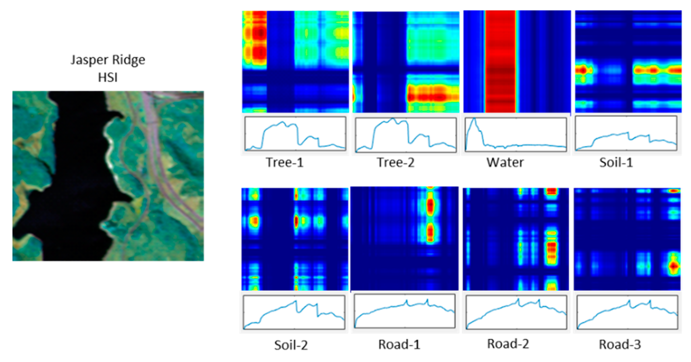
Figure 1 shows a CPD with eight components (R = 8). The original HSI has 198 bands and four endmembers. Components Tree-1 and Tree-2 have very similar spectral signatures but the optimization generates two components. Road-1, Road-2, and Road-3 show a similar issue where the road is split into three components. Constraining the optimization to R = 4 will produce the required number of components but there are not enough degrees of freedom to represent spatial features accurately.

Block Term Decomposition (BTD) is a generalization of CPD. It allows a tensor decomposition to be written as a sum of low-rank terms different than rank-1 [15]. Rank-(L, L, 1) in particular, is a 3-way decomposition specifying rank-L, with L > 1, for the first two dimensions and rank-1 for the third. The rank-(L, L, 1) can be expressed as:

$$Y={{\displaystyle \sum }}_{r=1}^R{F}_{\mathit{r}\colon\colon }^{\left(1\right)}{F}_{\mathit{r}\colon\colon }^{\left(2\right)T}\circ f_{r:}^{\left(3\right)}$$

(10)

where F⁽¹⁾ ∈ ${ℝ}^{R\times I_1\times L}$, F⁽²⁾ ∈ ${ℝ}^{R\times I_2\times L}$, and $f^{\left(3\right)} \in {ℝ}^{R\times I_3}$.

The motivation for using rank-(L, L, 1) decomposition stems from the characteristics of an HSI. Endmembers on a scene are in the order of one to ten; while spatial dimension sizes may be in the hundreds. This disparity can be addressed with rank-(L, L, 1) in such a way that fewer components are required to achieve a good spatial approximation.

3. Materials and Methods

3.1. Hyperspectral Data Sets

We experimented with three data sets widely used in academic literature for hyperspectral unmixing and classification. These data sets also have associated reference endmembers against which we will compare the capability of our approach. Here we provide a short description of the image content according to Le Sun’s website [16] where the data sets were downloaded from.

Samson is a simple image that contains water, trees, and soil. The Jasper Ridge image contains water, soil, trees, and roads. The Urban image contains grass, roads, buildings, and trees. There are three versions of ground truth for Urban containing 4, 5, and 6 endmembers. In our experiments, we tested with 4 and 6 endmebers.

Table 1. Dimensions of each HSI and number of reference endmembers, R.

HSI Set	I1, I2	I3	R
Samson	95, 95	156	3
J.Ridge	100, 100	198	4
Urban	307, 307	162	4, 6

shows the dimensions of hyperspectral input images.

3.2. Spatial Low-Rank Non-Negative Tensor Factorization Unmixing (SLR-NTF)

We propose using information from the spatial factors F⁽¹⁾ and F⁽²⁾, as shown in Equation (11), to extract endmembers which will later be used to generate abundance maps.

$$E_r=F_{\mathit{r}}^{\left(1\right)}{F}_{\mathit{r}}^{\left(2\right)T}$$

(11)

These factors multiplied the results in a spatial-low rank representation of the abundance of one particular spectral component, hence, the name Spatial Low-Rank NTF Unmixing (Supplementary Materials (SLR-NTF)). Having estimated endmembers, abundance maps are computed using the fully constrained least-squares (FCLS) [17].

Parameter R is set as the number of expected endmembers. We can also write Equation (7) in CPD form as a sum of LR components of rank-1. Hence, the resulting tensor is rank-LR, as shown in Equation (12):

$$Y={{\displaystyle \sum }}_{\mathit{r}}^{\mathit{R}}{{\displaystyle \sum }}_{\mathit{l}}^{\mathit{L}}\left(F_{\mathit{r}:\mathit{l}}^{\left(\mathbf{1}\right)}\circ F_{\mathit{r}:\mathit{l}}^{\left(\mathbf{2}\right)}\circ f_{:,\mathit{r}}^{\left(\mathbf{3}\right)}\right)$$

(12)

BTD is guaranteed to be essentially unique for a tensor with tensor rank LR ≤ min(I₁, I₂). However, HSIs are not guaranteed to have a tensor rank less than the size of their spatial dimensions. Since the rank is bounded by the total number of linearly independent components, we chose L proportional to the minimum size of the spatial dimensions and inversely proportional to R. Additionally, we weight L by the ratio of spatial to spectral size. This weight, min(I₁, I₂)/(I₃), adjusts L, increasing it when the spatial size is large relative to the spectral size and or reducing it when the opposite is true. An increase of spatial size relative to the spectral size would presumably increase the tensor rank assuming the spectral rank remains the same and is significantly smaller than the HS dimension. The calculation of L is shown in Equation (13):

$$L=\lfloor \frac{\mathbf{min}{\left(I_1,I_2\right)}^2}{R I_3}\rfloor$$

(13)

The selection of an optimal value of L based on signal unmixing continues to be a topic of research.

High magnitude regions on the spatial slab E_r, indicate a strong abundance of endmember r. Reconstructed pixels are selected from the regions where E_r/max(E_r) exceeds a threshold γ = 0.95. and the average of the selected pixels at those locations becomes the reconstructed endmember, as shown in Equation (14).

$$s_r={\displaystyle \sum }\frac{{\mathbf{Y}}^{’}\left(ar{g}_{i,j}\left(\frac{E_r,}{\max \left(E_r\right)}>\gamma \right),r\right)}{N}$$

(14)

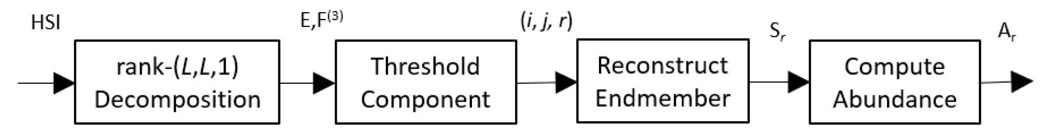
From the reconstructed endmembers, we compute the abundance of materials through FCLS. This method solves the least-squares inverse problem while applying the non-negativity constraint and the sum-to-one constraint imposed on the abundance map. Figure 2 shows a block diagram of the whole process.

3.3. Implementation on Tensorflow for GPU Execution

Tensorflow [18] uses an operation graph approach to perform multidimensional array computations with the goal of removing control logic from the programming model such that data can be streamed into vector processors with ease. The TensorFlow API abstracts low-level operations and implements hardware-specific vector, matrix, and tensor operations through runtime libraries optimized for the computing device. The code may run vector operations on multicore CPUs and take advantage of advanced vector processing instructions such as AVX and AVX2, using Intel’s Math Kernel Library, or OneAPI. GPUs between 10 and 100 times more functional units, which also take advantage of Tensor Flow’s framework. The same Tensorflow code can run on NVidia GPUs using the CUDA libraries and runtime. Pseudo code is shown on the section below and a full implementation and demo is available at: https://github.com/wilonavas/SLR-NTF.git.

Pseudocode for Spatial Low-Rank Tensor Factorization (SLR-NTF)

Inputs: = Source HSI Y, Number of endmembers R. Outputs: = Inferred Endmembers S’ = [s1, s2,.., sR], Abundance maps A’ = [A1, A2,… AR]

Estimate L $=\lfloor \frac{\mathbf{min}{\left(I_1,I_2\right)}^2}{R{I}_3}\rfloor$   Initialize $F^{\left(1\right)},F^{\left(2\right)},f^{\left(3\right)}$   Define computation graph for: Y’ = ${{\displaystyle \sum }}_{r=1}^R{F}_{\mathit{r}\colon\colon }^{\left(1\right)}{F}_{\mathit{r}\colon\colon }^{\left(2\right)T}\circ f_{r:}^{\left(3\right)}$   Define cost function: cost(Y, Y’) = $\left|\left|\mathrm{Y}-Y^{’}\right|\right|$   $\left(F^{\left(1\right)},F^{\left(2\right)},f^{\left(3\right)}\right)$ = Minimize(Cost(Y, Y’))   Compute Spatial Slices $E_r=F_{\mathit{r}}^{\left(1\right)}{F}_{\mathit{r}}^{\left(2\right)T}$   Extract endmembers ${\mathit{s}}_r={\displaystyle \sum }\frac{{\mathbf{Y}}^{’}\left(ar{g}_{i,j}\left(\frac{E_r,}{\max \left(E_r\right)}>\gamma \right),r\right)}{N}$   Compute abundance A’ = FCLS(Y’, S)

3.4. Initialization

SGD can be sensitive to initial conditions but heuristic methods have been developed to improve initialization and convergence. One of them is Glorot initialization [19]. It scales values on a narrow range that is inversely proportional to the factor sizes. There are two formulations. The first produces normally distributed random numbers with a standard deviation of σ = $\sqrt{2/M+N}$ where M and N are the input and output dimensions of a neural network layer. In our case, it is the dimensions of our factors. The second formulation is a random uniform distribution with numbers in the range $[-\sqrt{6}/\sqrt{M+N},\sqrt{6}/\sqrt{M+N}]$.

3.5. Optimizer

The rank-(L, L, 1) decomposition was implemented as a non-linear least-squares optimization problem solvable by the Stochastic Gradient Descent (SGD) family of methods. We leveraged existing frameworks for training neural networks and applied similar techniques for solving the rank-(L, L, 1) factorization problem. Numerical experiments by [20] show the non-linear methods are less sensitive to initial conditions and in some cases more robust than ALS. We used the Adam [21] optimizer included in Tensorflow. It required specifying a model, cost function, and setting appropriate stopping criteria based on reconstruction error. Below are the core functions used to implement the decomposition. Tensorflow primitives have the tf.* prefix. We removed the loops for iterating and stopping logic for clarity.

Optimizer Core functions

• def model(self):
  •    self.apply_anc(’relu’)
  •    op1 = tf.matmul(self.A,self.B,transpose_b=True)
  •    op2 = tf.tensordot(op1,self.C,[0,0])
  •    return op2
• def cost(self):
  •    se = tf.math.squared_difference(self.Y,model())
  •    mse = tf.reduce_mean(se)
  •    return mse
• def train(self, opt=tf.keras.optimizer.Adam):
  •    with tf.GradientTape() as tape:
          tape.watch(self.vars)
          curr_cost = self.cost()
  •    grads = tape.gradient(curr_cost,self.vars)
  •    opt.apply_gradients(zip(grads,self.vars))
  •    return curr_cost

The function model() defines the computation graph for the rank-(L, L, 1) decomposition using TensorFlow operations. We apply a Rectifier Linear Unit (ReLU) function to satisfy the abundance non-negative constraint. ReLU is simply set to zero any negative value that results from the application of the gradients.

With the function train(), we are leveraging the programming model commonly used for training neural networks to only perform tensor factorization. The GradientTape() performs automatic differentiation (AD) [22] and the optimizer applies changes to variables. In our case, the variables are the factors of the decomposition. The optimizer takes gradients as inputs, to dynamically adjust learning rate, momentum, and decay. Learning rate is the size of the steps by which weights are modified in the direction that most reduces the cost function. Large learning rates cause the error to oscillate around minimum while small learning rates require more iterations to reach a minimum.

Momentum in the context of SGD is analogous to having a ball with mass rolling down the cost function. The intent is to prevent the optimizer from converging on a shallow local minimum. If the optimizer reaches a minimum, it will tend to continue as long as it has momentum. Decay, following the physics analogy, is akin to friction. It uses an exponential function to reduce momentum in such a way that the descent reaches a “terminal speed” while going down a steep slope. Momentum dissipates if the surface is flat. These two considerations make Adam very effective in Deep Neural Network training and proved to be much faster and stable than SGD for our application.

The tensor operation op1 is a node in the TensorFlow compute graph. It computes the matrix multiplication of spatial factors F⁽¹⁾ and F⁽²⁾ resulting in spatial slices E_r. Then, op2 computes the sum of the outer products of spatial slices with spectral factors f⁽³⁾. Note that we use tensordot() to perform the outer product and contraction with a single call. However, below the high-level TensorFlow API, tensor fibers are being copied to the GPU’s memory where inner products are computed in parallel and sums of products are pipelined into specialized functional units such as CUDA cores and Tensor cores. In the case where we used the CPU, the operations are distributed amongst cores available and mapped to vector instructions such as AVX and AVX2.

3.6. Complexity and Performance

In this section, we discuss aspects of the asymptotic behavior of the proposed solution. We also present execution times for SLR-NTF algorithm running with an 8 core AMD Ryzen 3700 processor and compare it against an Nvidia RTX 3700GPU with 5888 CUDA cores.

The time complexity for one iteration of the optimizer is bound by some constant times the number of multiplications and additions done in Equation (10). If we let N ≥ max(I₁, I₂, I₃), and knowing L < min(I₁, I₂) and R << I₃, then the number of operations is asymptotically bound by O(N⁴). However, with R being much lower than the HSI dimensions (I₁, I₂, I₃), and L inversely proportional to R, it reduces to O(N³). We performed experiments with fixed size spectral dimension and verified O(N²) asymptotic behavior.

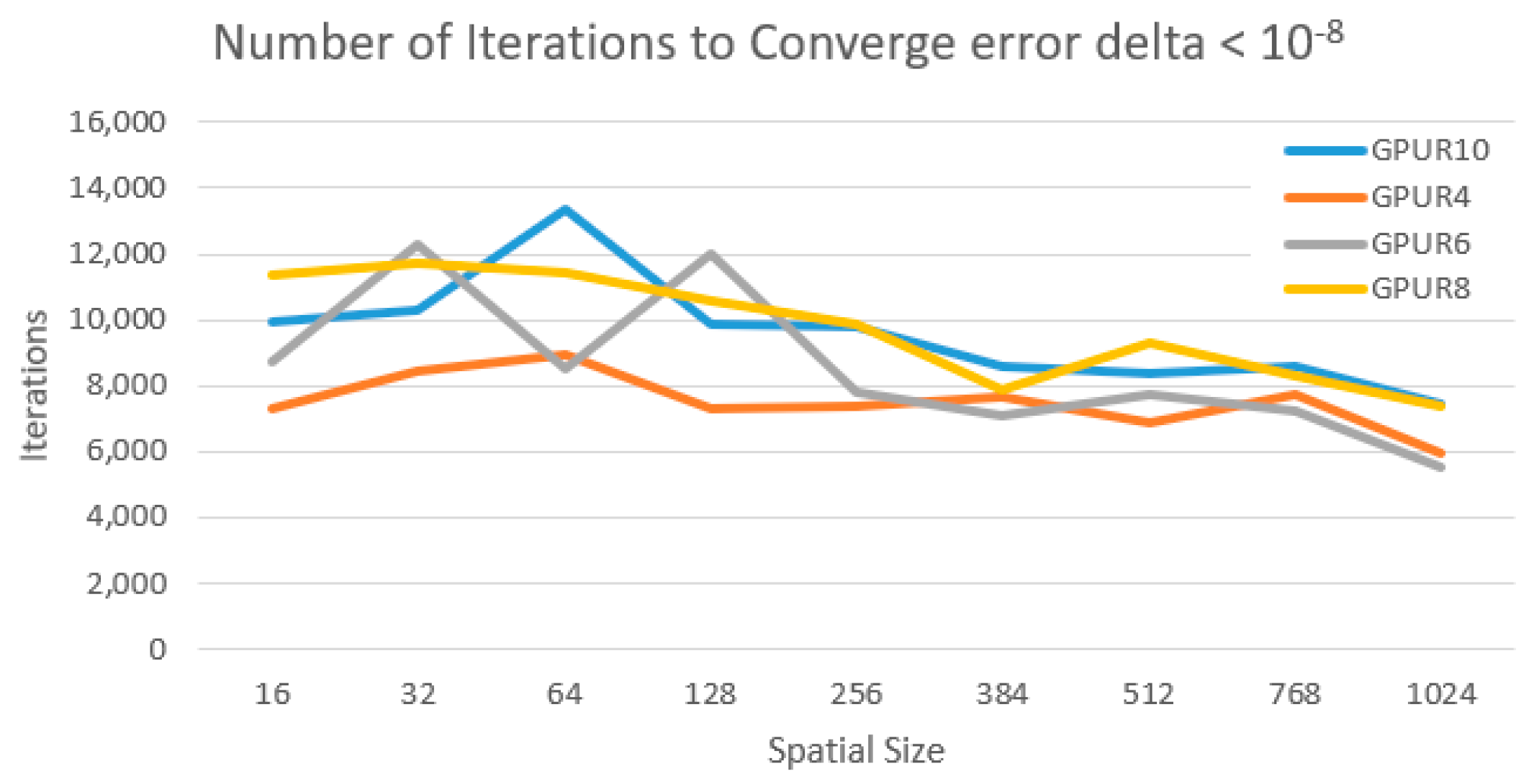
We ran the rank-(L, L, 1) decomposition to completion, measured iterations per second, and computed the time for a typical 10,000 iteration run. The 10,000 is an approximation of the number of iterations based on observed times, as shown in Figure 3.

To obtain experimental measurements, we generated a set of synthetic images with spatial dimensions (N = I₁, N = I₂) taking values of 16, 32, 64, 128, 256, 384, 512, and 1024. The spectral dimension was kept at I₃ = 220. We gathered the following observations:

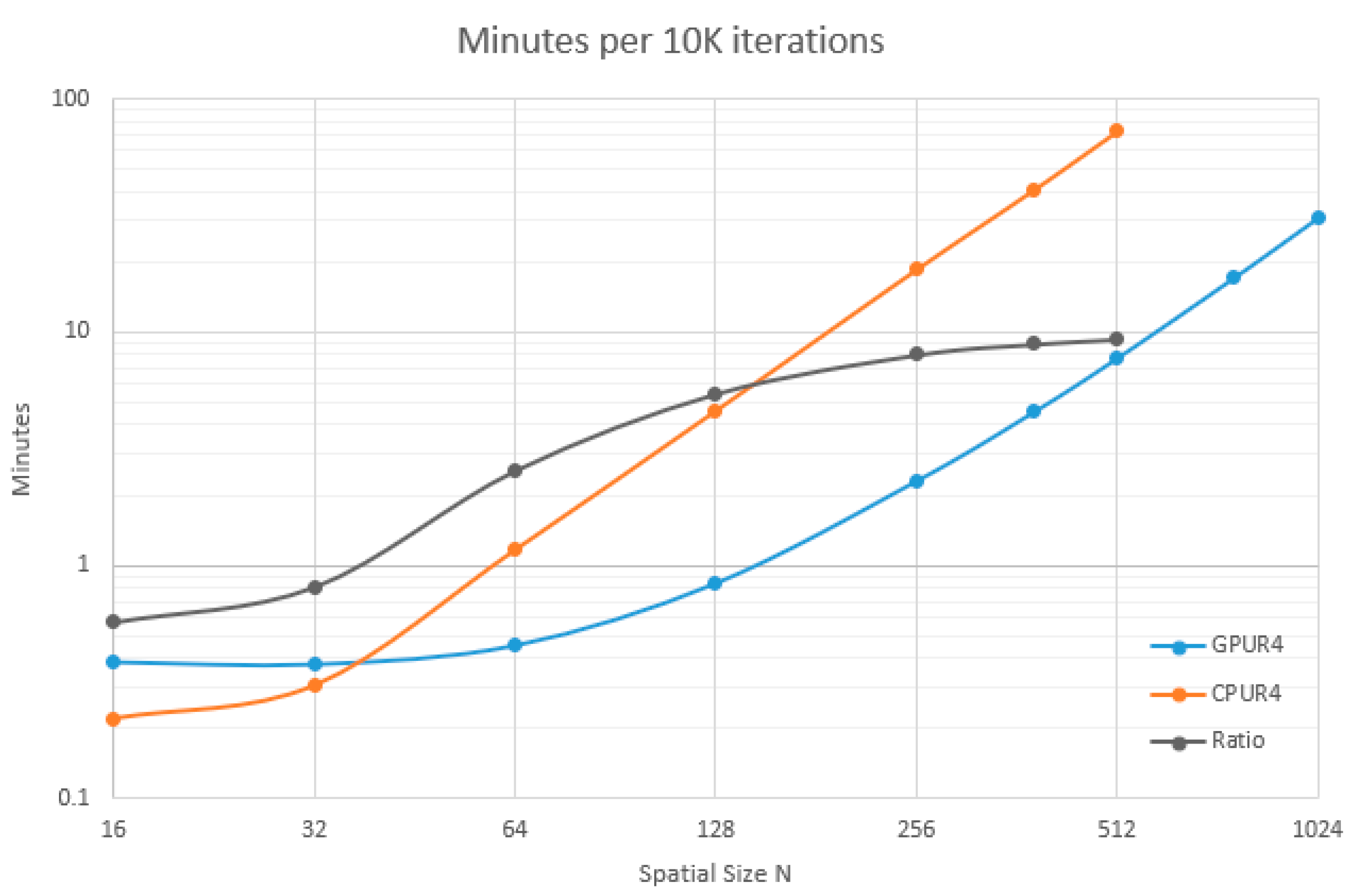
• Execution time on the CPU is faster than the GPU at sizes N < 32. It makes sense that communication overhead hurts GPU performance for small datasets. While the CPU has data in memory readily available for computation, the GPU has to send data across the PCI bus and get results back.
• The CPU exhibits linear time behavior in the range 16 < N < 32, and transitions to quadratic as N increases with a measured exponent of 1.96.
• GPU exhibits constant time behavior for N < 64. For N > 64, it slowly transitions to quadratic with a measured exponent of 1.95.
• The ratio between the CPU and GPU is the performance advantage, seen as the gray line on Figure 4. It increases and asymptotically approaches 10. In the range of N = 128 to N = 256, the GPU runs are from 5 to 8 times faster.
• The GPU implementation runs between 30 s and 2 min for images between N = 64 and N = 256. The CPU takes from 1 to 11 min for images in the same range.

4. Results

4.1. Performance Metrics

The root mean square error (RMSE) is a commonly used metric to measure average deviation of a predicted signal versus the actual data. It is the average magnitude of the residuals. Since the residuals are squared, it has the effect of weighting large differences more heavily than small ones. We will be using RMSE to measure the error of estimated abundance maps against reference ones provided with the datasets or computer generated in the case of synthetic images. The formulation for RMSE is shown in Equation (15):

$$RMSE\left(a_r,{a^{\prime }}_r\right)=\sqrt{\frac{1}{N}{{\displaystyle \sum }}_{n=1}^N{\left(a_r\left(n\right)-{a^{\prime }}_r\left(n\right)\right)}^2}$$

(15)

where a_r is the reference abundance and a’_r is the computed abundance for the rth endmember.

The spectral angle distance (SAD) is one of many metrics that measures similarity. It is related to the Pearson Correlation but operates on uncentered data. Geometrically it measures how much one vector is in the same direction of another, making it insensitive to changes in magnitude. Equation (16) shows the SAD computation:

$$SAD\left(\mathit{s},{\mathit{s}}^{\prime }\right)=\frac{<\mathit{s},{\mathit{s}}^{\prime }>}{\Vert \mathit{s}\Vert \Vert {\mathit{s}}^{\prime }\Vert }$$

(16)

where <∙,∙> denotes the inner product, s is the reference endmember, and s’ the computed one.

SGD is sensitive to initial conditions. Depending on the shape of the solution space, it can converge to a local minimum resulting in a suboptimal solution. In addition, the characteristics of the HSI along with the selection of the L parameter may not meet the requirements for uniqueness. For that reason, 10 runs for each set of parameters and inputs are executed. For each run, RSME and SAD are computed. Then, the mean and standard deviation for each set is reported as the final performance number.

4.2. Performance on Synthetic Images

In order to understand the behavior of SLR-NTF with different values of L, we tested synthetic images. The images were generated using the ”Hyperspectral Imagery Synthesis toolbox” [23]. The mean, standard deviation, and sum of mean and standard deviation for each metric is plotted. We expect to see less variation as the rank of the estimate approaches the rank of the original image, which should reflect as a minimum of the mean plus standard deviation.

Two input HSI sets were created. The first set, labelled “sleg-0x”, has abundance maps synthesized with Legendre low order polynomials. Figure 5 shows one HSI of the Legendre set. These polynomials produce smooth shapes with slowly changing gradients. The other set, labeled with prefix “sgau-0x”, creates abundance maps with random Gaussian fields, which produce more irregular content and material transitions. Figure 6 shows the first image of the Gaussian sets. All images are mixed spectral signature from the USGS Library [24]. Four minerals were chosen: Axinite HS342.3B, Brucite HS247.3B, Carnallite HS430.3B, and ChloriteHS179.3B. All images are 64 pixels wide by 64 tall and have 220 bands with a mixture of four endmember.

4.3. Legendre Synthetic HSI Results

The following series of plots are the results of SLR-NTF applied to the Legendre synthetic image set. We show the SAD and RMSE for choices of L = (2,4,8,16,24,32,48,56,64). For each value of L, five runs were made. The points on the plot correspond to the mean and standard deviation of SAD and RMSE.

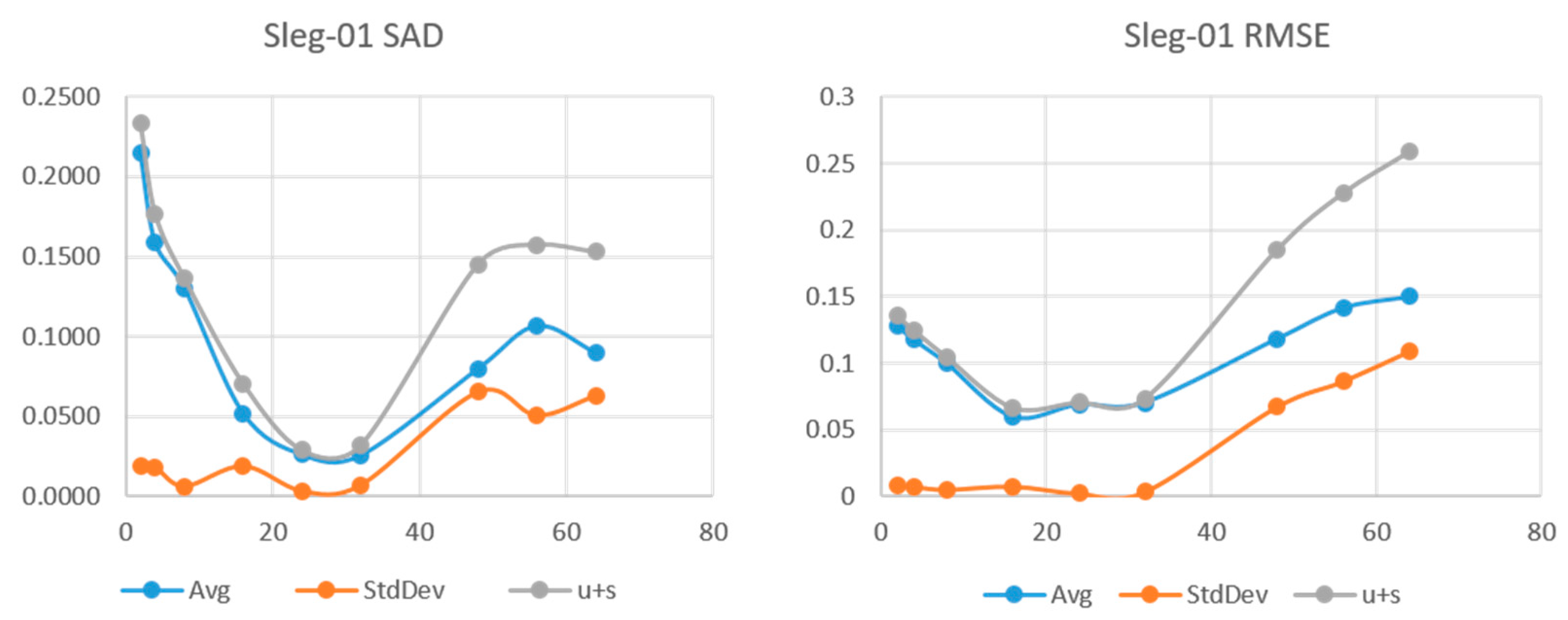
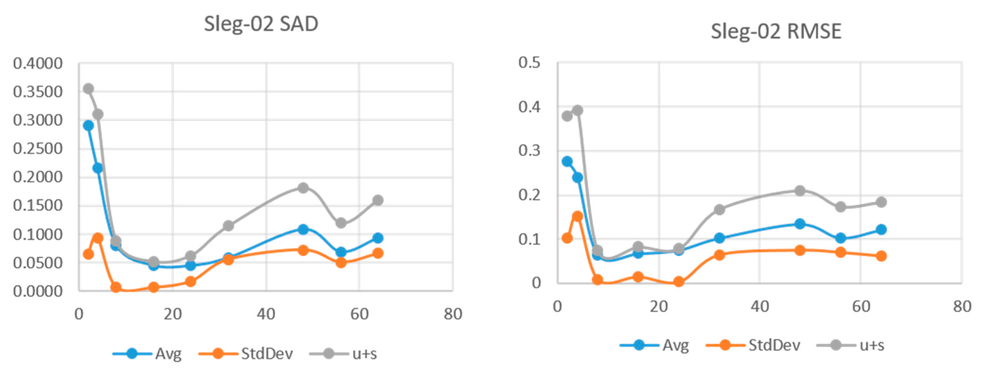
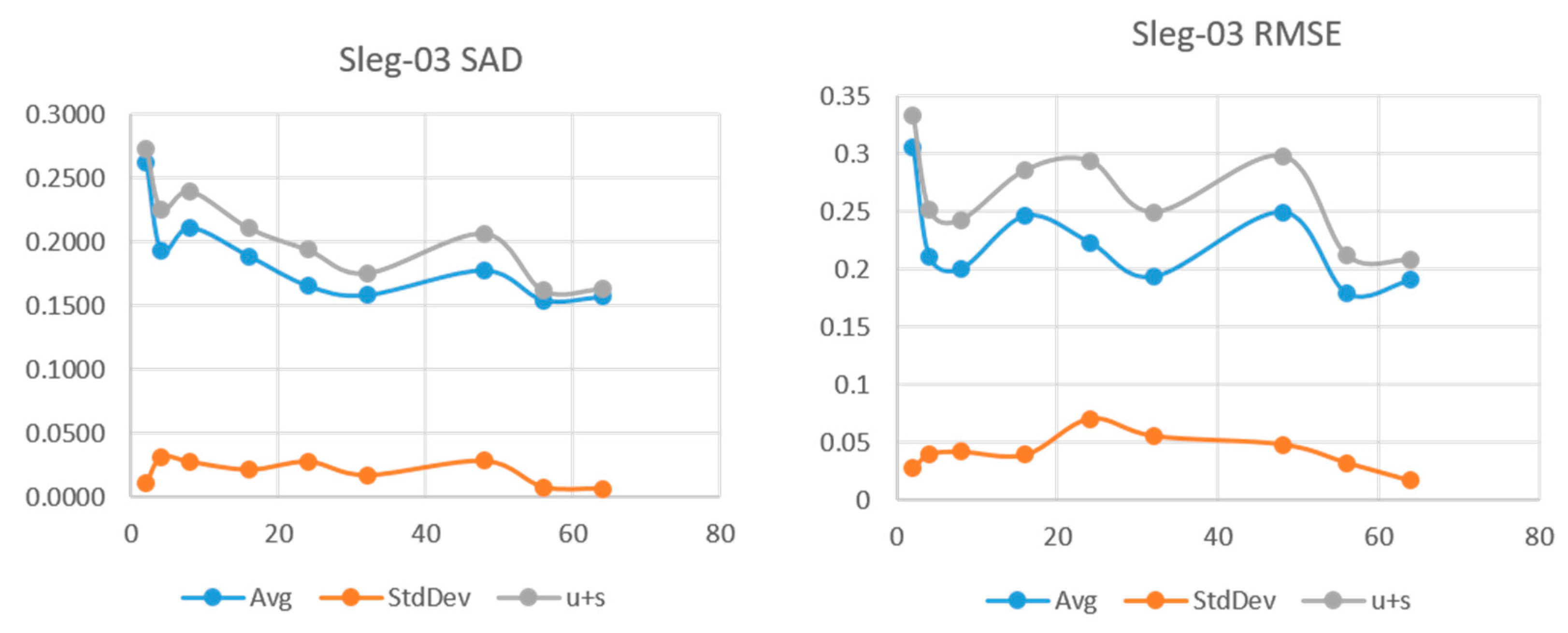
Figure 5, Figure 6 and Figure 7 show the results for the sleg-01, sleg-02, and sleg-03 HSI. We can see that sleg-01 and sleg-02 have a very low error and variability at L = 24 and L = 16, respectively. Sleg01 and Sleg02 show SAD in the range of 0.05 and more importantly, a very low standard deviation at that point. As L increases further, the variability of the runs increases, indicating we have augmented the degrees of freedom beyond the rank of the original HSI. Sleg03 has very small abundance of materials Axinite and Carnalite. In this case, the decomposition fails to make a good approximation of the endmembers for those low abundance regions. Figure 5, sleg-03 (b) and (c), shows very small abundances for materials Axinite and Carnalite, making them difficult to identify.

4.4. Gaussian Fields Synthetic HSI Results

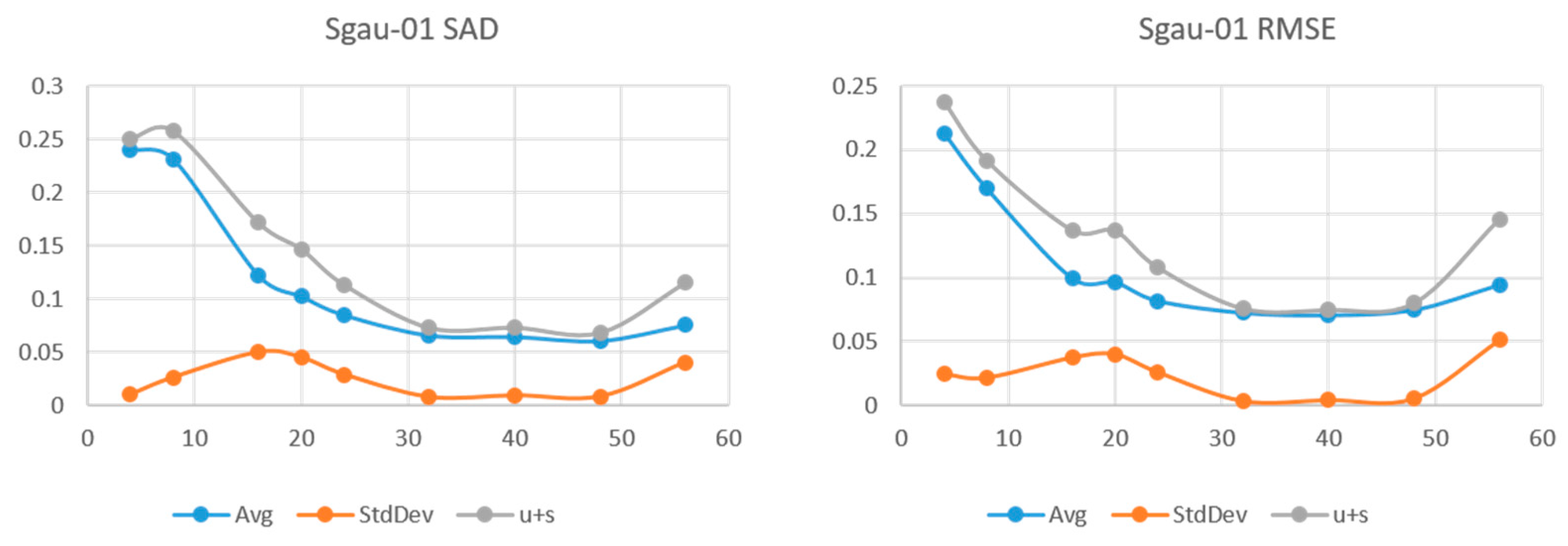
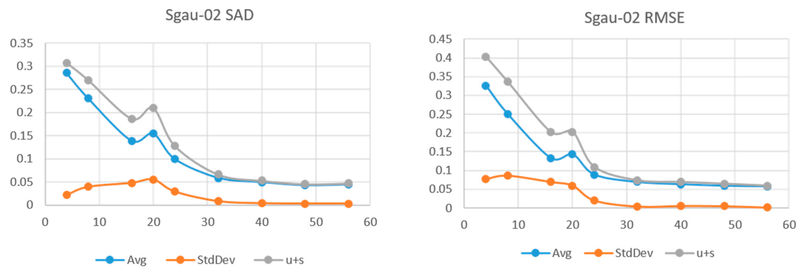
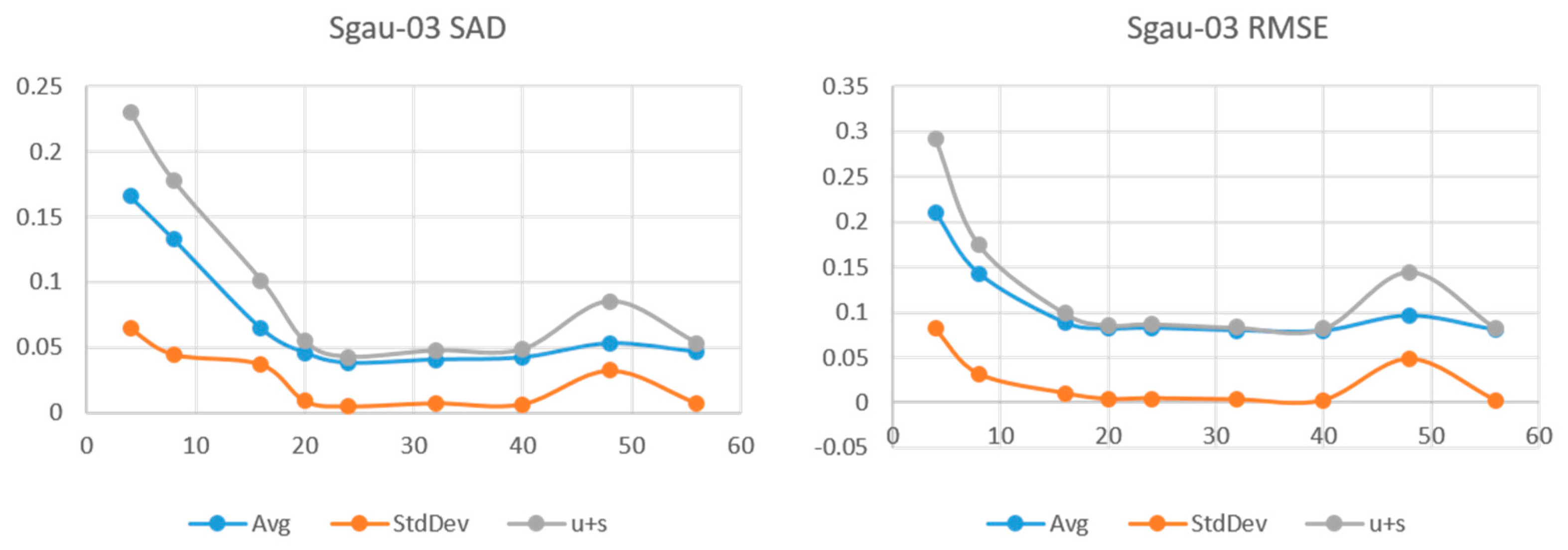
Results for the sgau set are shown on Figure 8, Figure 9 and Figure 10. For the sgau image set, we increased the number of trials to ten for each image and nine values of L were used. We see sgau-01 and sgau-02 reaching minimum SAD at L = 32, and sgau-03 at 20. Once at that point, variability is negligible with standard deviation an order of magnitude smaller than the mean. At the high end of the L values, sgau02 remains with low error and variability while sgau-01 and sgau-03 start increasing between 40 and 50. We can make a few observations from these results.

• The sleg set, being generated by low order polynomials, is smooth and the results confirm has a lower spatial rank than the sgau set.
• Both sets see very low variability when the representation has its lowest SAD and RMSE. We can infer that the solution is unique when the LR is close to the HSI tensor rank.
• In the “smooth” sleg images, using higher rank than necessary produces higher SAD and variability.

4.5. Performance on Real HSI Datasets

The benchmark measurements for SAD and RMSE were obtained from Y. Zhu [25]. The parameter L was set according to Equation (13) and R is set equal to the number of reference endmembers in the benchmark data set. We called our approach Spatial Low-Rank Non-negative Tensor Factorization and label it SLR-NTF. We compared our results for SLR-NTF against Vertex Component Analysis (VCA), NMF, NMF with l₁-norm and l_1/2-norm regularization, and matrix-vector NTF (MV-NTF), which is the only tensor-based approach included in the benchmark.

4.6. Samson Results

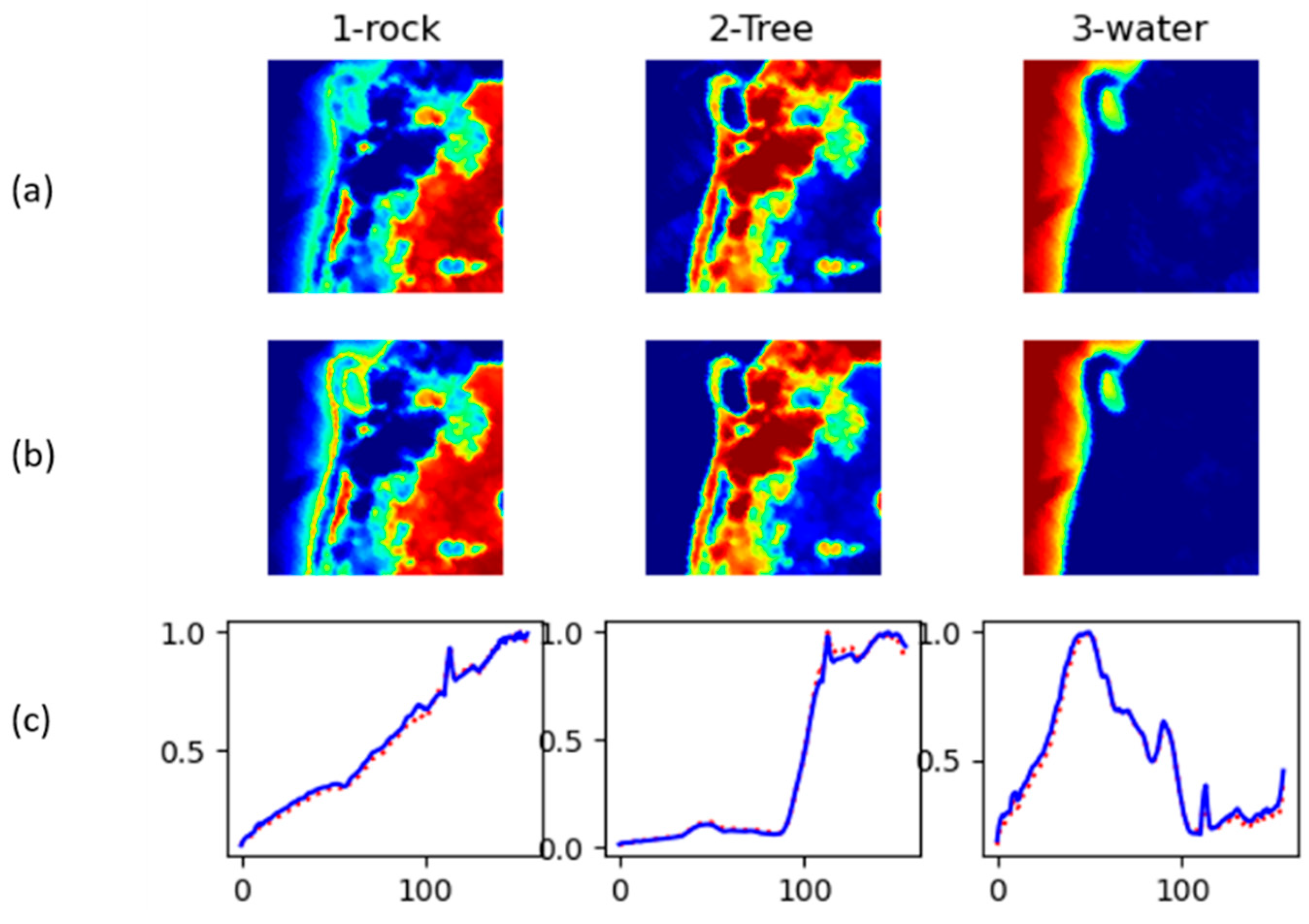
Samson results with the proposed method, SLR-NTF, are excellent. When comparing against the best result from other methods, in this case NMF-l₁, it is showing a 64% and 62% reduction in SAD and RMSE, respectively. As shown in

Table 2. Spectral Angle and RMSE Benchmarks for Samson.

	Spectral Angle Distance (SAD)					Root Mean Squared Error (RMSE)
	VCA	NMF	NMF-L1	NMF-L1/2	SLR-NTF	VCA	NMF	NMF-L1	NMF-L1/2	SLR-NTF
Soil	0.4239	0.2793	0.178	0.2074	0.0331	0.1504	0.1633	0.1425	0.1719	0.0546
Tree	0.1118	0.115	0.0542	0.0559	0.0343	0.1483	0.171	0.1341	0.1683	0.0388
Water	0.0662	0.0804	0.0778	0.0731	0.0414	0.1055	0.061	0.036	0.0395	0.0244
Avg.	0.2006	0.1582	0.1033	0.1121	0.0363	0.1543	0.1318	0.1042	0.1266	0.0393

, SAD with NMF-l_1/2 is 0.1033 vs. 0.0363 with SLR-NTF. The same for RMSE with results of 0.1042 for NMF-l_1/2 vs. 0.0244 for SLR-NTF. Figure 11 shows abundance maps and inferred endmembers for Samson.

4.7. Jasper Ridge Results

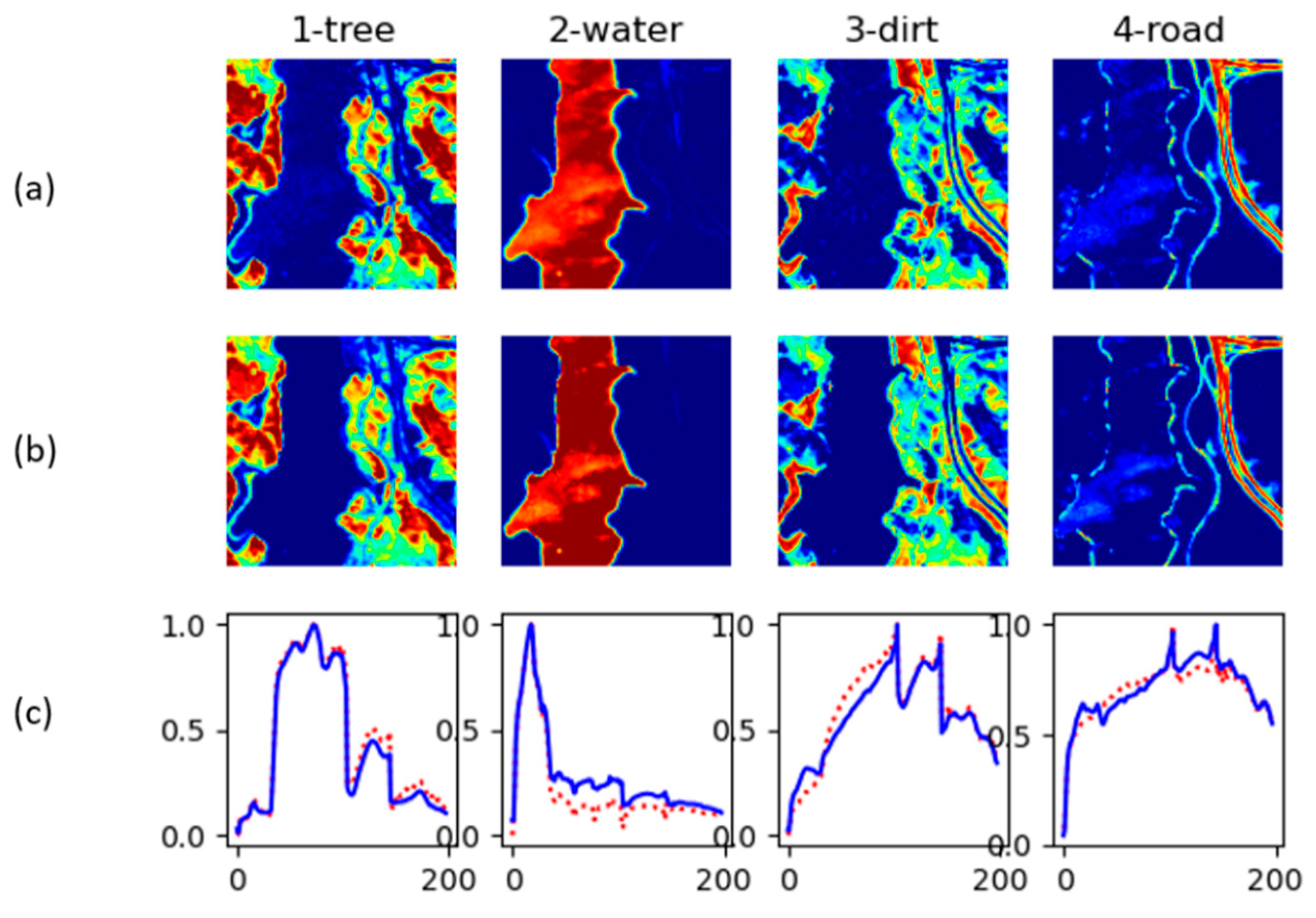
For Jasper Ridge, we obtained a SAD of 0.1115 and RMSE od 0.0609. The second best from the benchmark was NMF-L1/2 with RMSE of 0.1567 and RMSE of 0.1789. This translates to a reduction on RMSE of about 60% and 29% reduction for SAD when compared to NMF-L1/2.

Table 3. Spectral Angle and RMSE Benchmarks for Jasper.

	Spectral Angle Distance (SAD)					Root Mean Squared Error (RMSE)
	VCA	NMF	NMF-L1	NMF-L1/2	SLR-NTF	VCA	NMF	NMF-L1	NMF-L1/2	SLR-NTF
Tree	0.2565	0.2130	0.0680	0.0409	0.0714	0.3268	0.1402	0.0636	0.0707	0.0587
Water	0.2474	0.2001	0.3815	0.1682	0.2029	0.3151	0.1106	0.0660	0.1031	0.0387
Soil	0.3584	0.1569	0.0898	0.0506	0.1138	0.2936	0.2557	0.2463	0.2679	0.0798
Road	0.5489	0.3522	0.4118	0.3670	0.0581	0.2829	0.2450	0.2344	0.2737	0.0665
Avg.	0.3528	0.2305	0.2378	0.1567	0.1115	0.3046	0.1879	0.1526	0.1789	0.0609

shows the averages for SAD and RMSE for the different methods. Figure 12 shows abundance maps and inferred endmembers for Jasper Ridge.

4.8. Urban Results (4 Endmembers)

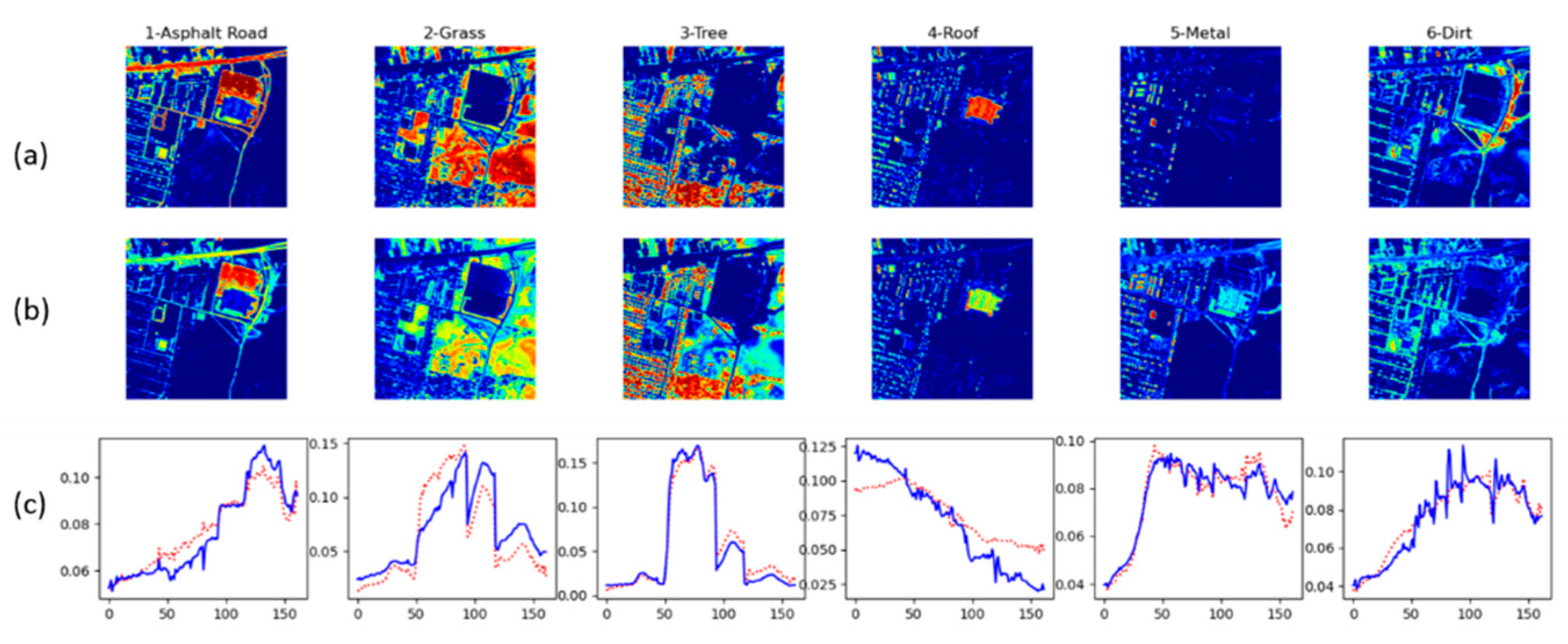
Unmixing on the Urban dataset produced SAD measurement of 0.1521 and RMSE of 0.1189. This image is the only one we could directly compare with another tensor decomposition (MV-NTF) approach with published results [11]. SLR-NTF achieves a SAD of 0.1521 and RMSE of 0.1521, as shown in

Table 4. Spectral Angle and RMSE Benchmarks for Urban (4 endmembers).

	Spectral Angle Distance (SAD)					Root Mean Squared Error (RMSE)
	NMF	NMF-L1	NMF-L1/2	MV-NTF	SLR-NTF	NMF	NMF-L1	NMF-L1/2	SLR-NTF
Asphalt	0.2114	0.1548	0.1349	0.1638	0.0774	0.2041	0.2279	0.3225	0.1226
Grass	0.3654	0.2876	0.099	0.2268	0.2176	0.2065	0.2248	0.3387	0.1320
Tree	0.1928	0.0911	0.0969	0.1054	0.0626	0.187	0.1736	0.2588	0.1438
Roof	0.737	0.7335	0.5768	0.3707	0.2507	0.1395	0.1861	0.1782	0.0772
Avg.	0.3168	0.2269	0.3778	0.2167	0.1521	0.1843	0.2031	0.2746	0.1189

. MV-NTF is the second best with a SAD with 0.2167 but a measurement for RMSE was not provided. NMF had the second best RMSE with 0.1842. In both cases, SLR-NTF was superior showing a SAD reduction of 30% against MV-NTF and an RMSE reduction of 35% reduction in RMSE. Figure 13 shows abundance maps and inferred endmembers for Urban with 4 endmembers.

4.9. Urban Results (6 Endmembers)

Table 5. Spectral Angle and RMSE Benchmarks for Urban (6 endmembers).

	Spectral Angle Distance					Root Mean Square Error (RMSE)
	VCA	NMF	NMF1	NMF1/2	SLR-NTF	VCA	NMF	NMF1	NMF1/2	SLR-NTF
Asphalt	0.2441	0.3322	0.2669	0.3092	0.0741	0.2555	0.2826	0.2803	0.3389	0.1626
Grass	0.3058	0.4059	0.3294	0.0792	0.2112	0.2696	0.3536	0.2937	0.2774	0.1414
Tree	0.6371	0.2558	0.2070	0.0623	0.1277	0.3212	0.2633	0.1859	0.2701	0.1323
Roof1	0.2521	0.3701	0.4370	0.0680	0.1643	0.2500	0.1662	0.1358	0.1541	0.0544
Metal	0.7451	0.6223	0.5330	0.1870	0.1297	0.2157	0.1603	0.2136	0.1660	0.1370
Soil	1.1061	0.9978	1.0371	0.0287	0.1044	0.2714	0.2505	0.2594	0.3542	0.2100
Avg	0.5484	0.4974	0.4684	0.1224	0.1352	0.2639	0.2461	0.2281	0.2601	0.1396

shows the results for the Urban dataset with six endmembers. Average SAD is 0.1352 for the endmembers and average RMSE for the abundance 0.1396. SAD decreased slightly compared with the 4 endmember decomposition. However, SLR-NTF has the second best SAD with NMF_1/2 being the best. Figure 14 shows abundance maps and inferred endmembers for Urban with six endmembers.

5. Conclusions and Future Work

In this work, we reviewed the use of non-negative tensor factorization for hyperspectral unmixing with particular attention to the use of spatial information.

Decomposition in the context of unmixing: the insights from CPD experiments motivated the use rank-(L, L, 1) decomposition, which provides better control of the spatial low rank, independent of the spectral rank. We introduced a workflow for spectral unmixing that directly uses spatial factors to infer endmembers and finally apply fully constrained least squares to obtain abundance maps.

We introduced a novel approach to use rank-(L, L, 1) decomposition for hyperspectral unmixing where the spatial factors are used to find candidate endmembers. As opposed to the CPD, the spatial factors of rank-(L, L, 1) have rank L independent from the number of components R. This overcomes the problem of limited detail on the spatial slice for each component, allowing for more accurate spatial representation. In experiments with synthetic images, it was shown that increasing the parameter L arbitrarily does not necessarily lead to the best factorization for unmixing. The non-negative rank-(L, L, 1) factorization is unique for LR equal to the original tensor rank. A tensor rank too low will produce poor approximations, while rank too high leaves the gradient descent based optimizer too many degrees of freedom; increasing the sensitivity to initial conditions. We proposed choosing a value of L that is proportional to the spatial dimensions and inversely proportional to R. The goal is for L to have just enough detail to represent regions of high abundance for one spectral component. We then use those regions to gather candidate endmembers for a given material from the low-rank reconstruction. The proposed method showed improved SAD and RMSE when applied to the Samson, Jasper Ridge, and Urban HSIs; as compared to other benchmarks in the same set.

It was also shown how TensorFlow was used for accelerating execution times on GPU vs. running on a multicore CPU and report how it scales for tensor sizes up to 1024 × 1024 × 220. In the range of N = 128 to N = 256, the GPU runs are from 5 to 8 times faster.

As future work, we consider building a neural network (NN) autoencoder that uses the rank-(L, L, 1) model as the decoder end. Hence, weight matrices of the NN are the tensor factors. The construction of the encoder is not trivial or unique. Other techniques used in Deep NN, such as drop-out and max-pooling are, in a way, reducing dimensionality and therefore rank. Exploration of a NN configuration of this type may lead to a novel way of estimating tensor rank.

References

- Landgrebe, D.A. Signal Theory Methods in Multispectral Remote Sensing; Wiley: Hoboken, NJ, USA, 2003. [Google Scholar]
- Sidiropoulos, N.D.; Lathauwer, L.D.; Fu, X.; Huang, K.; Papalexakis, E.E.; Faloutsos, C. Tensor Decomposition for Signal Processing and Machine Learning. IEEE Trans. Signal Process. 2017, 65, 3551–3582. [Google Scholar] [CrossRef]
- Qian, Y.; Xiong, F.; Zeng, S.; Zhou, J.; Tang, Y.Y. Matrix-Vector Nonnegative Tensor Factorization for Blind Unmixing of Hyperspectral Imagery. IEEE Trans. Geosci. Remote Sens. 2017, 55, 1776–1792. [Google Scholar] [CrossRef] [Green Version]
- Imbiriba, T.; Borsoi, R.A.; Bermudez, J.C.M. Low-Rank Tensor Modeling for Hyperspectral Unmixing Accounting for Spectral Variability. IEEE Trans. Geosci. Remote Sens. 2020, 58, 1833–1842. [Google Scholar] [CrossRef] [Green Version]
- Sun, L.; Wu, F.; Zhan, T.; Liu, W.; Wang, J.; Jeon, B. Weighted Nonlocal Low-Rank Tensor Decomposition Method for Sparse Unmixing of Hyperspectral Images. IEEE J. Sel. Topics Appl. Earth Obs. Remote Sens. 2020, 13, 1174–1188. [Google Scholar] [CrossRef]
- Xiong, F.; Qian, Y.; Zhou, J.; Tang, Y.Y. Hyperspectral Unmixing via Total Variation Regularized Nonnegative Tensor Factorization. IEEE Trans. Geosci. Remote Sens. 2019, 57, 2341–2357. [Google Scholar] [CrossRef]
- Keshava, N.; Mustard, J.F. Spectral Unmixing. IEEE Signal Process. Mag. 2002, 19, 44–57. [Google Scholar] [CrossRef]
- Nascimento, J.M.P.; Bioucas-Dias, J.M. Hyperspectral Signal Subspace Estimation. In Proceedings of the 2007 IEEE International Geoscience and Remote Sensing Symposium, Barcelona, Spain, 23–27 July 2007; pp. 3225–3228. [Google Scholar]
- Donoho, D.; Stodden, V. When Does Non-Negative Matrix Factorization Give a Correct Decomposition into Parts? In Advances in Neural Information Processing Systems 16; Thrun, S., Saul, L.K., Schölkopf, B., Eds.; MIT Press: Cambridge, MA, USA, 2004; pp. 1141–1148. [Google Scholar]
- Zhou, G.; Cichocki, A.; Zhao, Q.; Xie, S. Nonnegative Matrix and Tensor Factorizations : An Algorithmic Perspective. IEEE Signal Process. Mag. 2014, 31, 54–65. [Google Scholar] [CrossRef]
- Qian, Y.; Jia, S.; Zhou, J.; Robles-Kelly, A. Hyperspectral Unmixing via L1/2Sparsity-Constrained Nonnegative Matrix Factorization. IEEE Trans. Geosci. Remote Sens. 2011, 49, 4282–4297. [Google Scholar] [CrossRef] [Green Version]
- Kolda, T.G.; Bader, B.W. Tensor Decompositions and Applications. SIAM Rev. 2009, 51, 455–500. [Google Scholar] [CrossRef]
- Tucker, L.R. Some Mathematical Notes on Three-Mode Factor Analysis. Psychometrika 1966, 31, 279–311. [Google Scholar] [CrossRef] [PubMed]
- Sidiropoulos, N.D.; Bro, R. On the Uniqueness of Multilinear Decomposition of N-Way Arrays. J. Chemom. 2000, 14, 229–239. [Google Scholar] [CrossRef]
- Lathauwer, L. Block Component Analysis, a New Concept for Blind Source Separation; Springer: Berlin/Heidelberg, Germany, 2012; Volume 7191, pp. 1–8. [Google Scholar]
- Sun, L. Hyperspectral Data Sets. Available online: http://lesun.weebly.com/hyperspectral-data-set.html (accessed on 4 June 2021).
- Heinz, D.C. Chein-I-Chang Fully Constrained Least Squares Linear Spectral Mixture Analysis Method for Material Quantification in Hyperspectral Imagery. IEEE Trans. Geosci. Remote Sens. 2001, 39, 529–545. [Google Scholar] [CrossRef] [Green Version]
- Abadi, M.; Barham, P.; Chen, J.; Chen, Z.; Davis, A.; Dean, J.; Devin, M.; Ghemawat, S.; Irving, G.; Isard, M.; et al. TensorFlow: A System for Large-Scale Machine Learning. In Proceedings of the 12th USENIX Symposium on Operating Systems Design and Implementation, Savannah, GA, USA, 2–4 November 2016. [Google Scholar]
- Glorot, X.; Bengio, Y. Understanding the Difficulty of Training Deep Feedforward Neural Networks. J. Mach. Learn. Res. Proc. Track 2010, 9, 249–256. [Google Scholar]
- Sorber, L.; Van Barel, M.; De Lathauwer, L. Optimization-Based Algorithms for Tensor Decompositions: Canonical Polyadic Decomposition, Decomposition in Rank-$(L_r,L_r,1)$ Terms, and a New Generalization. SIAM J. Optim. 2013, 23, 695–720. [Google Scholar] [CrossRef] [Green Version]
- Kingma, D.P.; Ba, J. Adam: A Method for Stochastic Optimization. In Proceedings of the 5th International Conference on Learning Representations, Toulon, France, 24–26 April 2017. [Google Scholar]
- Baydin, A.G.; Pearlmutter, B.A.; Radul, A.A.; Siskind, J.M. Automatic Differentiation in Machine Learning: A Survey. J. Mach. Learn. Res. 2018, 18, 1–43. [Google Scholar]
- Grupo de Inteligencia Computacional. Hyperspectral Imagery Synthesis (EIAs) Toolbox; Universidad del País Vasco/Euskal Herriko Unibertsitatea: Spain, Leioa, 2021. [Google Scholar]
- Kokaly, R.F.; Clark, R.N.; Swayze, G.A.; Livo, K.E.; Hoefen, T.M.; Pearson, N.C.; Wise, R.A.; Benzel, W.M.; Lowers, H.A.; Driscoll, R.L.; et al. USGS Spectral Library Version 7; Data Series; US Geological Survey: Reston, VA, USA, 2017; p. 68.
- Zhu, F. Spectral Unmixing Datasets with Ground Truths. CoRR. 2017. abs/1708.05125. Available online: https://www.researchgate.net/profile/Feiyun-Zhu-2/publication/319164320_Spectral_Unmixing_Datasets_with_Ground_Truths/links/59a84536a6fdcc2398387589/Spectral-Unmixing-Datasets-with-Ground-Truths.pdf (accessed on 4 June 2021).
Figure 1.
Components of a CPD computed for the Jasper Ridge HSI using CPD with R = 8. The false color plots correspond to the magnitude of Er (red is larger), and the plot below each slab is the spectral factor, fr(3).