WiFi-Aided Magnetic Matching for Indoor Navigation with Consumer Portable Devices

Abstract

This paper presents a WiFi-aided magnetic matching (MM) algorithm for indoor pedestrian navigation with consumer portable devices. This algorithm reduces both the mismatching rate (i.e., the rate of matching to an incorrect point that is more than 20 m away from the true value) and computational load of MM by using WiFi positioning solutions to limit the MM search space. Walking tests with Samsung Galaxy S3 and S4 smartphones in two different indoor environments (i.e., Environment #1 with abundant WiFi APs and significant magnetic features, and Environment #2 with less WiFi and magnetic information) were conducted to evaluate the proposed algorithm. It was found that WiFi fingerprinting accuracy is related to the signal distributions. MM provided results with small fluctuations but had a significant mismatch rate; when aided by WiFi, MM’s robustness was significantly improved. The outcome of this research indicates that WiFi and MM have complementary characteristics as the former is a point-by-point matching approach and the latter is based on profile-matching. Furthermore, performance improvement through integrating WiFi and MM depends on the environment (e.g., the signal distributions of magnetic intensity and WiFi RSS): In Environment #1 tests, WiFi-aided MM and WiFi provided similar results; in Environment #2 tests, the former was approximately 41.6% better. Our results supported that the WiFi-aided MM algorithm provided more reliable solutions than both WiFi and MM in the areas that have poor WiFi signal distribution or indistinctive magnetic-gradient features.

1. Introduction

While Global Navigation Satellite Systems (GNSS) based outdoor navigation has greatly advanced over the past few decades, positioning and navigation in indoor and deep urban areas are still open issues [1]. The challenges include unavailable or degraded GNSS signals, complex indoor environments, necessity of using low-grade devices, etc. Wireless positioning technologies have been applied to provide long-term absolute positions [2]. Especially, as WiFi receivers are ubiquitous in consumer devices such as smartphones, it is feasible to implement WiFi positioning in public areas with existing WiFi infrastructures. WiFi fingerprinting approaches based on received signal strengths (RSS) have gained a large amount of attention, as they can provide position without any knowledge of the access point (AP) location or signal-propagation model [3]. However, the utilization of WiFi requires the creation and maintenance of a network. Furthermore, RSS fluctuate significantly due to obstructions, reflections [4], and multipath effects [5]. Fluctuations of RSS have limited the promotion of wireless positioning technologies [6].

Advances in Micro-Electro-Mechanical Systems (MEMS) technology have made it possible to produce chip-based sensors, such as inertial sensors (i.e., accelerometers and gyros) and magnetometers. MEMS sensors have become appropriate candidates for motion tracking and navigation applications because they are small and lightweight, consume little power, and are extremely low-cost [7]. Especially, inertial sensors are ideal for providing continuous information in indoor/outdoor environments because they are not dependent on the transmission or reception of signals from an external source [8]. However, inertial sensors provide only short-term accuracy and suffer from accuracy degradation over time due to the existence of sensor errors [9]. Calibration is a useful way to remove many deterministic sensor errors and improve sensor-based navigation [10]; however, MEMS inertial sensors suffer from significant run-to-run biases and thermal drifts [11]. Especially, the heading error will grow when there is no aiding information [12]. Magnetometers can assist the heading estimation by sensing the geomagnetic field [13]. Nevertheless, the local magnetic field is susceptible to interferences from man-made infrastructure in indoor or urban environments [14], which makes magnetometer-derived heading angle unreliable. Magnetic interference is a critical issue when magnetometers are used as a compass indoors.

However, the indoor magnetic interference can also be exploited as an advantage by leveraging the magnetic abnormalities as fingerprints [15,16]. The magnetic matching (MM) approach has been proposed based on the hypothesis that the indoor magnetic field is stable over time and non-uniform (i.e., changes significantly) with location [17,18]. MM is achieved in two phases (steps): The offline training (pre-survey) phase and the online positioning phase. The training phase is conducted to build or update a “location, magnetic intensity” database (DB) that consists of a set of reference points (RPs) with known coordinates and the magnetic intensity on these RPs, while the positioning step is implemented to find the closest match between the features of the measured magnetic intensity and those stored in the DB. While MM utilizes a similar idea to WiFi fingerprinting, it is independent from any infrastructure, as the magnetic field is omnipresent. The challenge for MM is that magnetic data only consists of three components. Because the heading is generally unknown, it is only feasible to extract two components with the help of accelerometers, i.e., vertical magnetic intensity and horizontal magnetic intensity (or total magnetic intensity and inclination). To increase the magnetic fingerprint dimension without extra sensors, the profile-matching method has been proposed [19]. A sequence of observations are saved in the memory and then compared with the candidate profiles stored in the DB. There are well-developed profile-matching methods such as terrain contour matching (TERCOM) [18,19] and iterative closest contour point (ICCP) [20]. To obtain the optimal match, the profile length should be long enough to show the profile feature; moreover, the length of the measured profile should be the same as that of the stored profiles. However, for indoor cases, sensors are low-end and there is no effective constraint if the device is not fixed on the body (e.g., on-foot or in-belt). Thus, the sensor-based navigation error will accumulate quickly and make it difficult to measure the accurate moving distance [21]. In this paper, we calculate the rough length of the measured profile using the steps detected by accelerometers. Because accurate and real-time step-length estimation is still an open issue in pedestrian navigation, we utilize the dynamic time warping (DTW) algorithm for matching with inaccurate profile length [22].

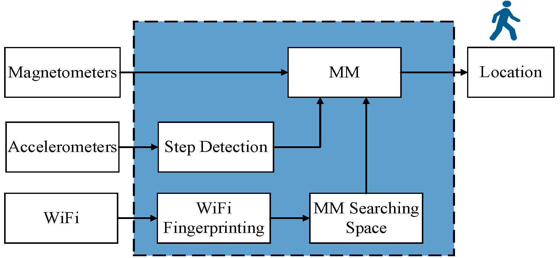
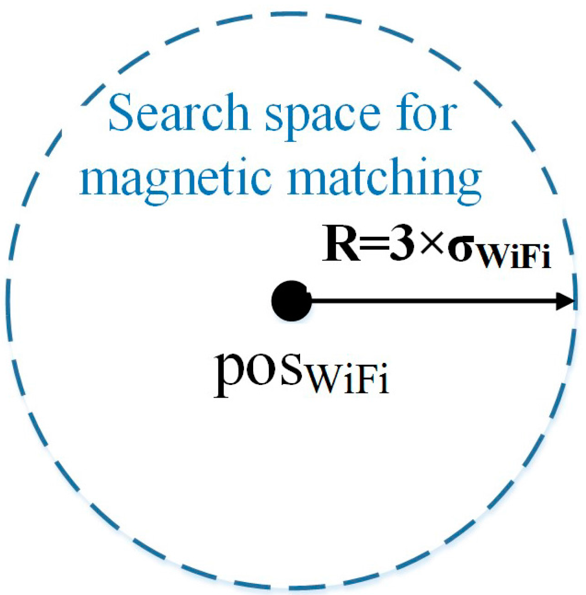
This paper presents a WiFi-aided MM navigation algorithm that uses off-the-shelf sensors in consumer portable devices and existing WiFi infrastructures. The basic idea is using WiFi results to limit the MM search space, so as to reduce both the mismatching rate and the computational load. This algorithm was designed after comparing WiFi and MM, and taking advantage of the merits of each technology. We found that MM results had small error fluctuations but had a significant mismatch rate (i.e., the rate of matching to an incorrect point that was more than 20 m away from the true value). In contrast, WiFi fingerprinting can provided results with low mismatch rate; however, the WiFi fingerprinting accuracy strongly depended on the signal distributions. Finally, the proposed WiFi-aided MM provided more reliable results than either the independent use of WiFi or MM and had a lower mismatch rate.

The paper is organized as follows: Section 2 outlines the architecture of the WiFi-aid magnetic matching algorithm and a detailed description of each component; Section 3 investigates the navigation performance of different technologies; and Section 4 draws the conclusions.

2. WiFi-Aided Magnetic Matching Algorithm

The block diagram of the algorithm architecture is shown in Figure 1. This section first describes the principle of magnetic matching and WiFi fingerprinting, and then it introduces the WiFi-aided magnetic matching algorithm.

Figure 1. Algorithm architecture.

Figure 1. Algorithm architecture.

MM and WiFi fingerprinting utilize similar ideas and both consist of the training phase and the positioning phase. This section introduces these two phases separately.

2.1. Training Phase for WiFi Fingerprinting and Magnetic Matching

The purpose of training is to build or update a “location, RSS” DB and a “location, magnetic intensity” DB. The key to generating reliable DBs is obtaining accurate RP coordinates. The choice of the DB training method is a trade-off between cost and accuracy. Different training approaches have been researched according to various requirements. The first approach is to survey at every RP and record its fingerprint. This point-by-point method can improve the DB reliability by averaging the measurements (RSS or magnetic intensity) at each RP [23] and even provide a rough estimate of orientation [24]. However, it is time- and labor-consuming when dense RPs are selected to cover an entire area of interest, and a surveyor needs to mark the position of all RPs manually [25]. The point-by-point training can take up to several hours even for a small building [26].

To reduce the time and labor costs, we adopt the walk-survey method. The walk-survey method is used based on landmarks (i.e., points with known coordinates) or floor plans (i.e., the true positions of corners and intersections and the true orientation of corridors) and a constant-speed assumption. A surveyor has to walk with a constant speed along each link between landmarks, such as corners or intersections, over the pre-designed path. The positions of landmarks are determined on a digital map, while those of other RPs and the links between landmarks are calculated by the arrival time and the distance between landmarks. Although the DB generated by walk-survey tends to be less accurate than that from the point-by-point approach, walk-survey is significantly more time-effective. Furthermore, with inertial sensors on smartphones, we utilize the steps detected by accelerometers to replace the constant-speed assumption by a constant-step-length assumption, and we use the heading changes calculated from gyros to remove the requirement for straight walking. The procedure of training and positioning is shown in Figure 2.

Figure 2. Procedure of training phases for magnetic matching and WiFi fingerprinting.

Figure 2. Procedure of training phases for magnetic matching and WiFi fingerprinting.

Magnetometers on smartphones have a higher sampling rate (commonly more than 10 Hz). Therefore, we store every step as a RP. Furthermore, we assume that the device moves with a constant speed within each step; thus, we calculate the magnetic intensity at a set of points within this step through interpolation. The interpolated points are also stored as MM RPs. The MM fingerprint at the k-th RP is recorded as:

$$F{M}_k=\left\{po{s}_k,{\sigma }_{posk},m_k\right\}$$

(1)

where pos_k and σ_posk are the location of RP_k and its accuracy, m_k is the magnetic intensity vector at RP_k. The approach for determining the σ_pos values is related with the DB training method used. According to the DB training method we use, we calculate the value σ_pos for the step points on the i-th link (or arc) by ${\sigma }_{pos,p}=\frac{\alpha \cdot L_i}{N_i}$, where L_i is the length of the i-th link, N_i is the number of steps on this link, and α is a scale factor. σ_pos is an optional parameter. If there is no σ_pos in the fingerprints, all RPs have the same weight in the DB. The fingerprints on the interpolated points between two adjacent step points (e.g., m₁ and m₂) are set by the following method: Assuming the fingerprints at m₁ and m₂ are FM_m1 and FM_m2, and there are n interpolated points between m₁ and m₂, then the fingerprints at the i-th interpolated point is $F{M}_{m1}+\frac{i}{n+\text{1}}(F{M}_{m2}-F{M}_{m1})$, where $1\le i\le n$.

In general, more elements in each fingerprint are better for matching. With accelerometers on smartphones, we detect the roll and pitch angles and in turn extract the vertical and horizontal magnetic intensities. The roll and pitch angles are calculated as:

$$\begin{array}{l}\mathrm{\varphi }=a\tan 2(-f_y,-f_z)\\ \mathrm{\theta }=a\tan 2(f_x,\sqrt{f_y^2+f_z^2})\end{array}$$

(2)

where Φ and θ are the roll and pitch angles, f_i (i = x, y, z) is the accelerometer-measured specific force along the i-th axis.

We can transfer the magnetic vector in body-frame (i.e., the magnetometer measurements) to that in navigation frame (i.e., the local magnetic vector) by using [27]:

$$B^n=C_b^n{B}^b$$

(3)

where $C_b^n$ is the direction cosine matrix (DCM), which can be represented by the roll, pitch, and heading angles as:

$$C_b^n=\left[\begin{array}{ccc}\mathrm{c}\mathrm{\theta }c\mathrm{\psi }& -\mathrm{c}\mathrm{\varphi }\mathrm{s}\mathrm{\psi }+\mathrm{s}\mathrm{\varphi }\mathrm{s}\mathrm{\theta }\mathrm{c}\mathrm{\psi }& \mathrm{s}\mathrm{\varphi }\mathrm{s}\mathrm{\psi }+\mathrm{c}\mathrm{\varphi }\mathrm{s}\mathrm{\theta }\mathrm{c}\mathrm{\psi }\\ \mathrm{c}\mathrm{\theta }\mathrm{s}\mathrm{\psi }& \mathrm{c}\mathrm{\varphi }\mathrm{c}\mathrm{\psi }+\mathrm{s}\mathrm{\varphi }\mathrm{s}\mathrm{\theta }\mathrm{s}\mathrm{\psi }& -\mathrm{s}\mathrm{\varphi }\mathrm{c}\mathrm{\psi }+\mathrm{c}\mathrm{\varphi }\mathrm{s}\mathrm{\theta }\mathrm{s}\mathrm{\psi }\\ -\mathrm{s}\mathrm{\theta }& \mathrm{s}\mathrm{\varphi }\mathrm{c}\mathrm{\theta }& \mathrm{c}\mathrm{\varphi }\mathrm{c}\mathrm{\theta }\end{array}\right]$$

(4)

where Ψ is the heading angle. s and c are the shorthand notations of sin( ) and cos( ), respectively.

Let $B^b={\left[\begin{array}{ccc}{B}_x& B_y& B_z\end{array}\right]}^T$ and $B^n={\left[\begin{array}{ccc}{B}_N& B_E& B_D\end{array}\right]}^T$, the vertical magnetic intensity can be calculated by:

$$B_D=-\sin \mathrm{\theta }\cdot B_x+\sin \mathrm{\varphi }\cos \mathrm{\theta }\cdot B_y+\cos \mathrm{\varphi }\cos \mathrm{\theta }\cdot B_z$$

(5)

Therefore, we construct the magnetic intensity vector as $m=\left[\begin{array}{ccc}B& B_D& B_H\end{array}\right]$, where $B=\left|B^b\right|$ is the total magnetic intensity, and $B_H=\sqrt{B^2-B_D^2}$ is the horizontal magnetic intensity.

Compared with WiFi, android smartphones commonly have low WiFi update rates (e.g., approximate 0.3 Hz for Samsung Galaxy smartphones). Thus, we combine the RSS and the coordinates of the latest step as a fingerprint when the RSS is updated. The WiFi fingerprint at the i-th RP is recorded as:

$$\begin{array}{c}F{W}_i=\{po{s}_i,{\sigma }_{posi},\left(ma{c}_{i,1},RS{S}_{i,1}\right),\\ \left(ma{c}_{i,2},RS{S}_{i,2}\right),\cdots ,\left(ma{c}_{i,m_i},RS{S}_{i,m_i}\right)\}\end{array}$$

(6)

where pos_i and σ_posi are the coordinate of RP_k and its accuracy, mac_i,j and RSS_i,j are the MAC address and RSS of the j-th AP received at RP_i, and m_i is the number of available APs at RP_i.

2.2. Positioning Phase for WiFi Fingerprinting and Magnetic Matching

MM is a profile-matching method, while WiFi fingerprinting is based on point-by-point matching. Therefore, these two techniques are described separately.

2.2.1. Magnetic Matching

The basic idea of MM is calculating the difference between the measured profile and the candidate profiles in the DB, and finding the best match. The “match” can be indicated by the minimum value of a given formula such as mean absolute difference (MAD) [19]:

$$MAD=\frac{1}{N}{\displaystyle \sum _{i=1}^N\left|S_i-M_i\right|}$$

(7)

where S_i is the measured profile, M_i is the profile in the DB, and N is the profile length.

To obtain the optimal match, the profile length should be long enough to show the profile feature; additionally, it is preferred that the length of the measured profile and the candidate profile should be the same. We utilize the steps detected by accelerometers to calculate the rough length of the measured profile. Because accurate and real-time step-length estimation is still an open issue in pedestrian navigation, we use the dynamic time warping (DTW) algorithm, which is originally used in the speech recognition area, for matching with inaccurate profile length.

The technique in DTW [22] is to compress or stretch the time axis of one (or both) sequences to achieve a better alignment. The goal is to find the best match between two sequences, $S=\left\{s_1,s_2,\mathrm{...},s_A\right\}$ and $M=\left\{m_1,m_2,\mathrm{...},m_B\right\}$, of different lengths. The best match is found by obtaining the optimal warping path w. The warping path is given by $w=w(1),w(2),\mathrm{...},w(n)$, where $w(i)=[i(n),j(n)]$ is a set of matched samples, where i and j are the time-axes of two sequences, respectively. The objective of the warping function is to minimize the overall cost function given by $D={\displaystyle \sum _{n=1}^N\mathrm{\delta }(w(n))}$, where ${\displaystyle \sum _{n=1}^N\delta (w(n))}={(i(n)-j(n))}^2$ is the squared distance between the sample points.

To generate a warping path, a cost matrix is constructed. This matrix represents the minimum cost required to reach a particular point (i, j) from (1, 1). This minimization problem is usually solved using the dynamic programming approach, whereby a cumulative distance γ (i, j) is computed as the sum of the distance obtained from the current set of points $\mathrm{\delta }(w(n))$ and the minimum of the cumulative distances of the adjacent elements or neighbors by:

$$\gamma (i,j)=\mathrm{\delta }(w(n))+\min [\gamma (i-1,j),\gamma (i-1,j-1),\gamma (i,j-1)]$$

(8)

2.2.2. WiFi Fingerprinting

The user location is estimated by finding the closest match between the measured RSS vector with those stored in the DB. The most typical WiFi fingerprinting approaches are the Nearest Neighbor (NN) method and the probabilistic estimation approach [28]. The NN method selects the RP that has the minimal signal strength distance as the user’s estimated position by using [23]:

$$d_i=|S{S}_{rec,l_u}-S{S}_{DB,i}|,i\in I_{RP}$$

(9)

where, d_i is the signal strength distance at RP_i, l_u is the position to be determined, $S{S}_{rec,l_u}$ is the measured RSS vector at l_u, SS_DB,i is the RSS vector at RP_i, and I_RP is the location index set of RPs in the DB. After this, the location of RP_i which satisfies the condition $d_{i^{*}}=\min (d_i|i\in I_{RP})$ is determined as the position estimate of l_u.

To mitigate the impact of blunders and obtain a more reliable position, the k-NN method is considered [29]. The k-NN method estimates the position according to the k RPs that have the smallest distances. The position estimate is obtained by a weighed sum of the position of these RPs by:

$$\widehat{r}={\displaystyle \sum _{i=1}^k\frac{c_i}{C}}{r}_i$$

(10)

where $c_i=1/d_i$, $C={\displaystyle \sum _{i=1}^k{c}_i}$, $r_i$ is the position of the i-th nearest RP, and $\widehat{r}$ is the estimated position.

2.2.3. WiFi-Aided Magnetic Matching

Compared with WiFi, MM results have smaller fluctuations but more mismatches. Thus, we use WiFi positioning result to limit the MM search space to reduce both the mismatch rate and the computational load. The search space is limited to a circle around the WiFi results, as shown in Figure 3. The radius of the circle is set according to the WiFi accuracy.

Furthermore, a multi-level quality control mechanism is applied to make WiFi solutions robust. The first level is on WiFi fingerprinting. Several methods are used to detect WiFi blunders. The first is on the measurement level, where a threshold value Th_RSS is set to filter out APs with weak RSS. The second is based on the minimal signal strength distance. If the minimal signal strength distance at a certain epoch is larger than the value Th_d1, the WiFi results at this epoch will be regarded as a point outside the DB.

Figure 3. Using WiFi positioning results to limit search space for magnetic matching.

Figure 3. Using WiFi positioning results to limit search space for magnetic matching.

This methodology can also be extended to Bluetooth or other techniques. Since Bluetooth can be used in a similar way as WiFi (either fingerprinting or trilateration), it is feasible to use Bluetooth to determine a region first, and then use magnetic matching to determine the position. When both WiFi and Bluetooth are available, both a WiFi result and a Bluetooth result can determine a region. If this is the case, the position uncertainty of the integrated use of WiFi and Bluetooth can be smaller than that of the independent use of WiFi or Bluetooth. Accordingly, the position accuracy can be further improved.

Tests and results of WiFi, MM, and WiFi-aided MM are demonstrated in Section 3.

3. Tests and Analysis

Two sets of tests were conducted at the University of Calgary, one on the main floor of the Energy Environment Experiential Learning (EEEL) building, and the other is on the lower main floor of the Engineering building (ENB). These two buildings were chosen because they have different types of indoor environments. EEEL is a relatively new building with well-equipped infrastructure. Accordingly, there are more WiFi APs (the average number of RSS was over 15 in this building) and severe magnetic interferences (the change of magnetic intensity reached 0.4 Gauss). In contrast, the lower main floor of ENB is mainly used for walking; thus, there are less APs (the average number of RSS was nearly seven) and less magnetic interferences (the change of magnetic intensity was below 0.25 Gauss). The sizes of tested areas in EEEL and ENB were around 120 × 40 m² and 140 × 60 m², respectively. The tests were performed with Samsung Galaxy S3 and S4 (S3 for training and S4 for positioning) smartphones. We conducted the tests in this paper with the handheld mode to focus on the hybrid navigation.

3.1. Tests at EEEL

3.1.1. Training Phase

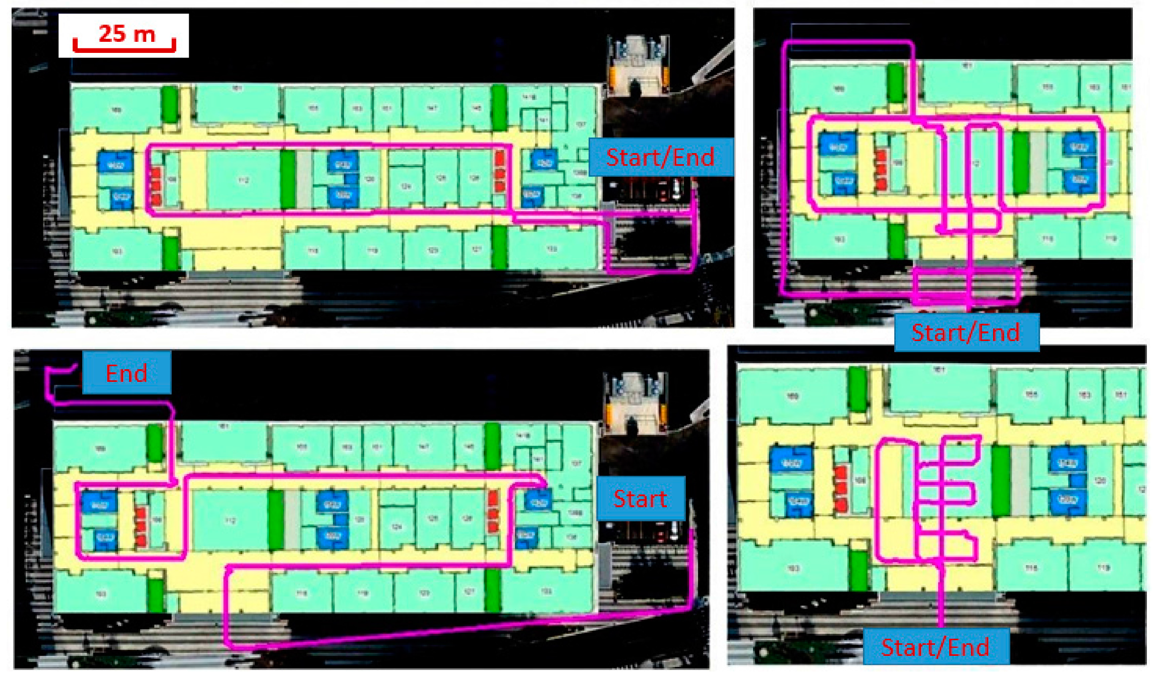
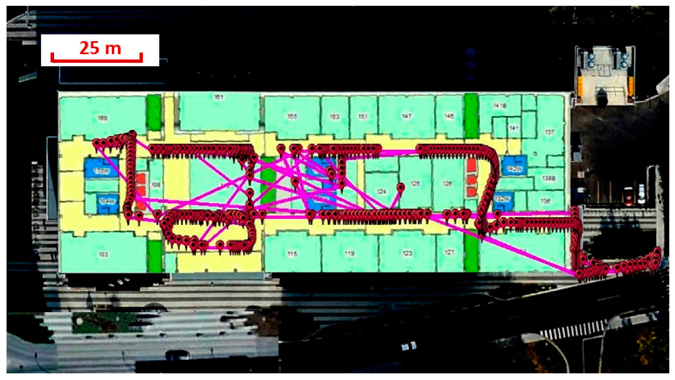
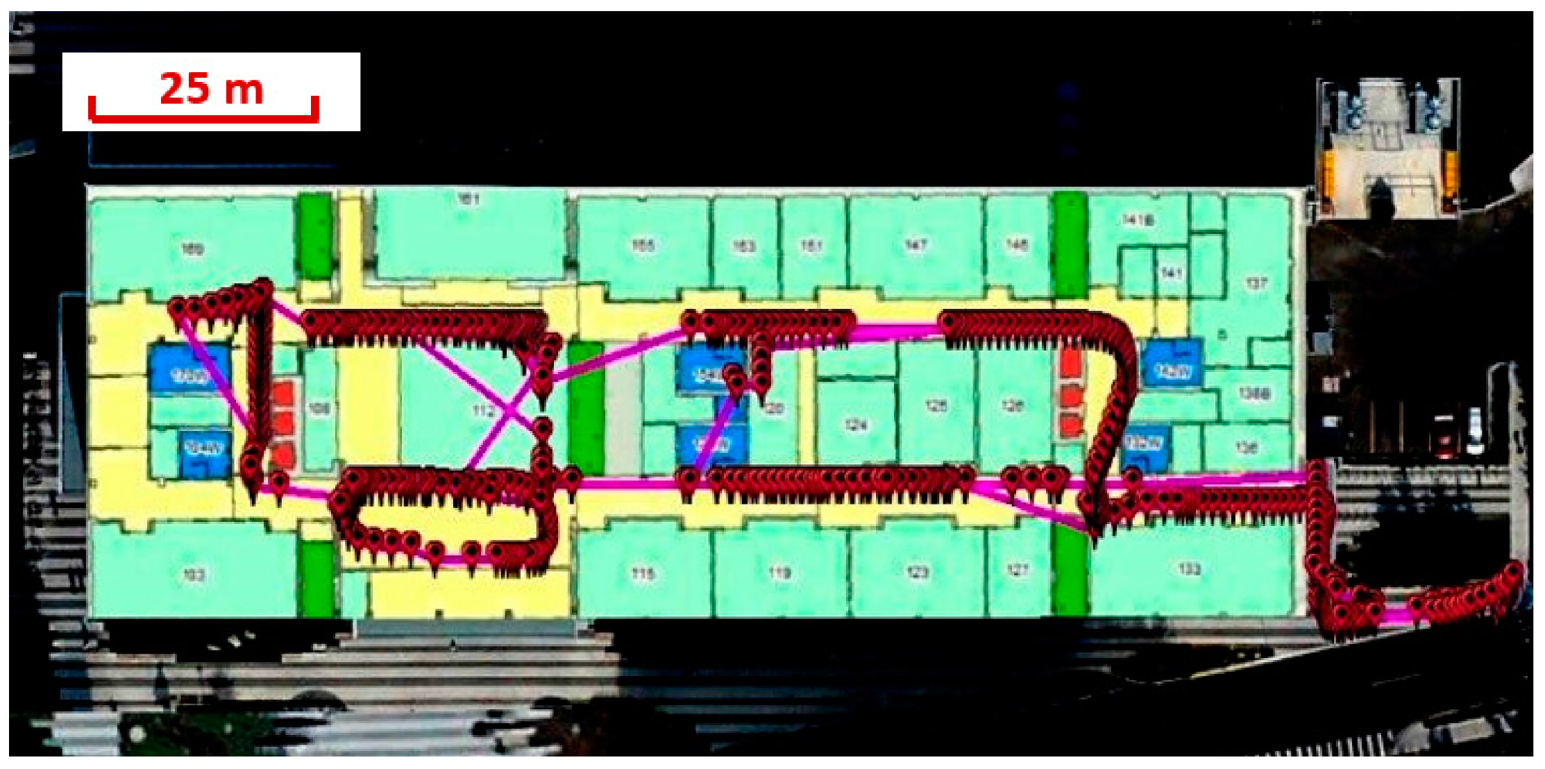
We generated the magnetic and WiFi DBs inside the EEEL building using four different trajectories. The true trajectories are shown in Figure 4. Each trajectory lasted for 5–10 min. The coordinates of the landmarks (i.e., the start and end points and corners and intersections) and the orientations of corridors were obtained from Google Earth and utilized as constraints to generate the DBs.

Figure 4. Trajectories used to generate WiFi and magnetic databases (DBs) at the Energy Environment Experiential Learning (EEEL).

Figure 4. Trajectories used to generate WiFi and magnetic databases (DBs) at the Energy Environment Experiential Learning (EEEL).

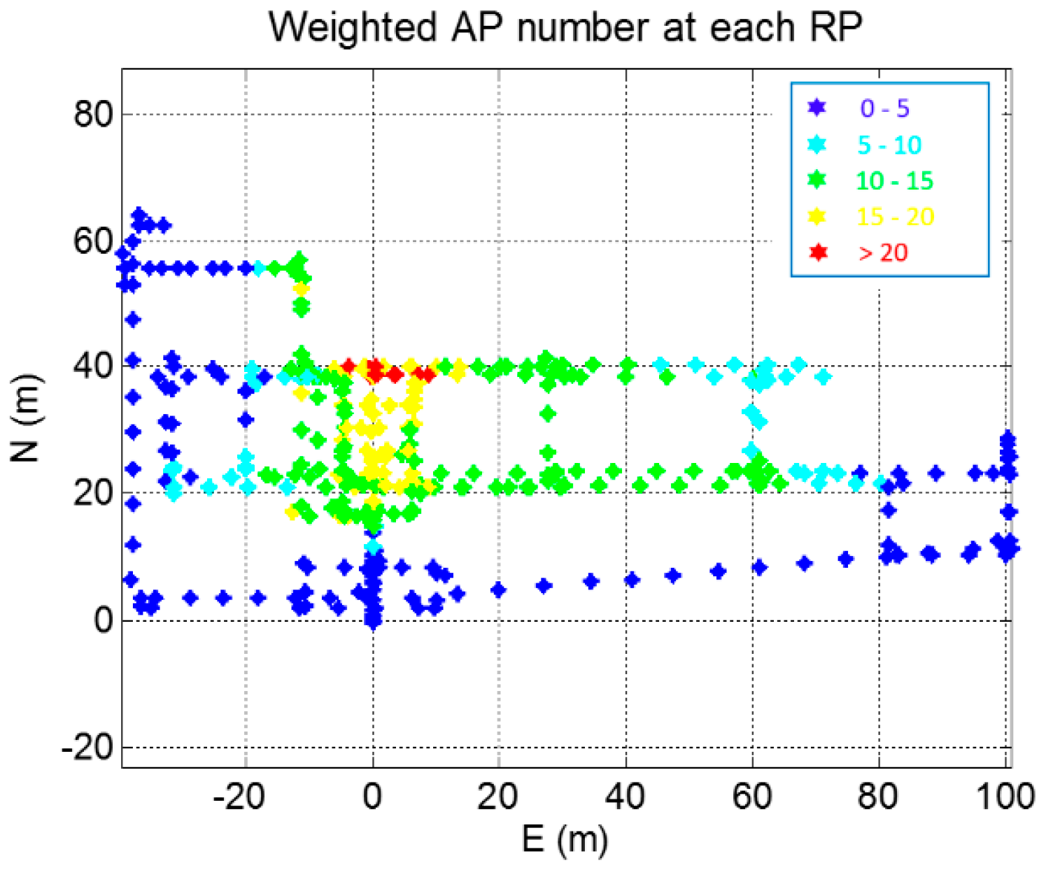
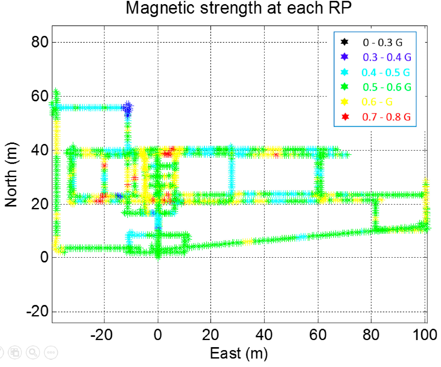
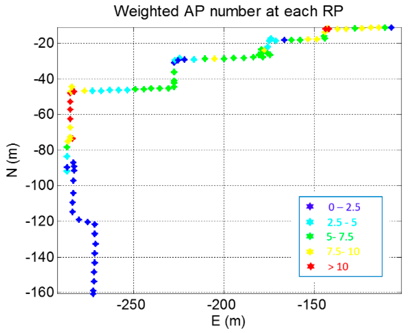
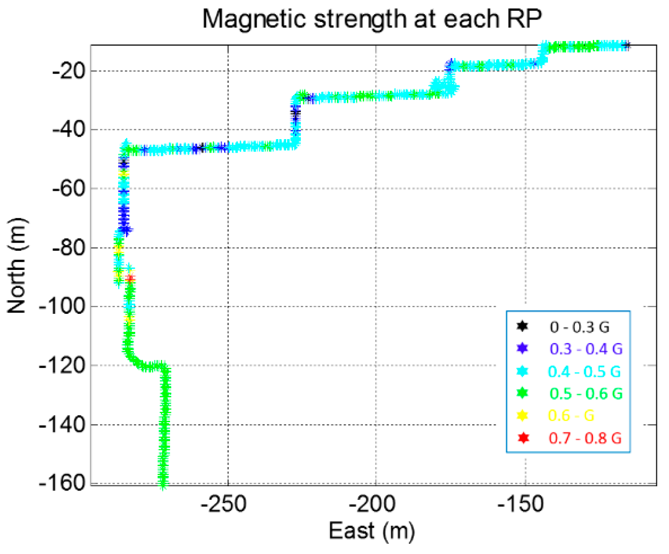
When the WiFi RSS information was updated, it was combined with the coordinate of the surveyor’s latest step as a fingerprint only. The WiFi update rate on tested smartphones was about 0.3 Hz; thus, the distance between two WiFi RPs was approximate 3 m. The RPs in the magnetic DB included all steps and interpolation points. The interpolation distance was set at 0.1 m. The scale factor α was set at 0.2. The RPs in the WiFi and magnetic DBs are shown in Figure 5 and Figure 6, respectively. The x- and y-axes indicate the length in the west–east and south–north directions. The colors in Figure 5 and Figure 6 indicate the weighted AP number and the magnetic strength. Over 15 RSS were available in the middle indoor area, and over 10 were available in the marginal indoor areas. The magnetic intensity varied from 0.3 Gauss to 0.8 Gauss indoors. The weighted AP number at RP_i was calculated by:

$$WA{P}_i={\displaystyle \sum _{j=1}^{n_i}{a}_{i,j}},i\in I_{RP}$$

(11)

where n_i is the number of WiFi signals received at RP_i, I_RP is the location index set of RPs in the DB. The value of a_i,j is determine according to RSS_i,j (i.e., the RSS of AP_j at RP_i) by the following rule: If RSS_i,j > −60 dBm, a_i,j = 1; else, if −70 dBm < RSS_i,j < −60 dBm, a_i,j = 0.75; else, if −85 dBm < RSS_i,j < −70 dBm, a_i,j = 0.25; else, if RSS_i,j < −85 dBm, a_i,j =0.

Figure 5 shows that the available WiFi signals were abundant in the middle area of EEEL, less in the marginal indoor areas, and even less in outdoor areas. Figure 6 indicates that the magnetic intensity was within 0.5–0.6 G (the geomagnetic intensity at Calgary is 0.57 G) at most of the outdoor RPs; however, the magnetic intensity varied significantly indoors.

Figure 5. WiFi signal distribution at EEEL.

Figure 5. WiFi signal distribution at EEEL.

Figure 6. Magnetic distribution at EEEL.

Figure 6. Magnetic distribution at EEEL.

3.1.2. Positioning Phase

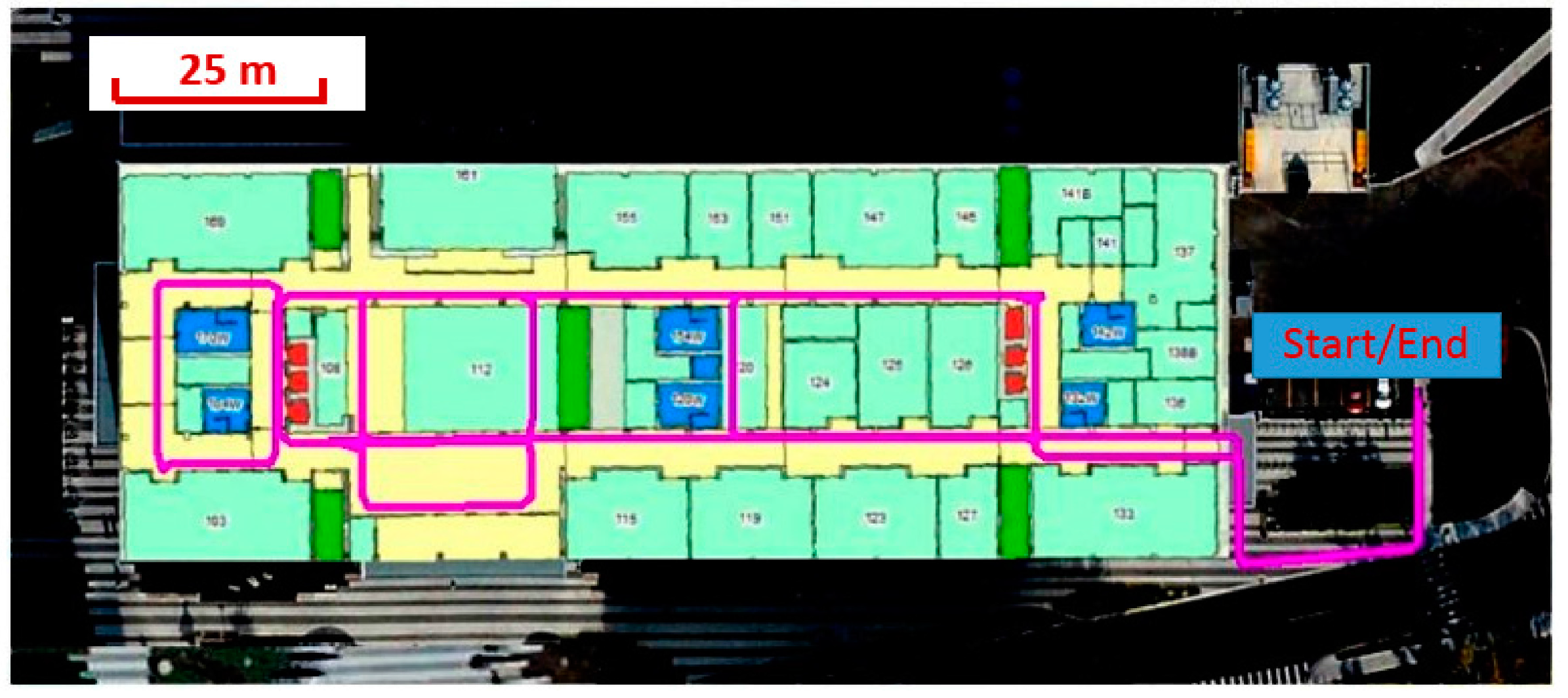
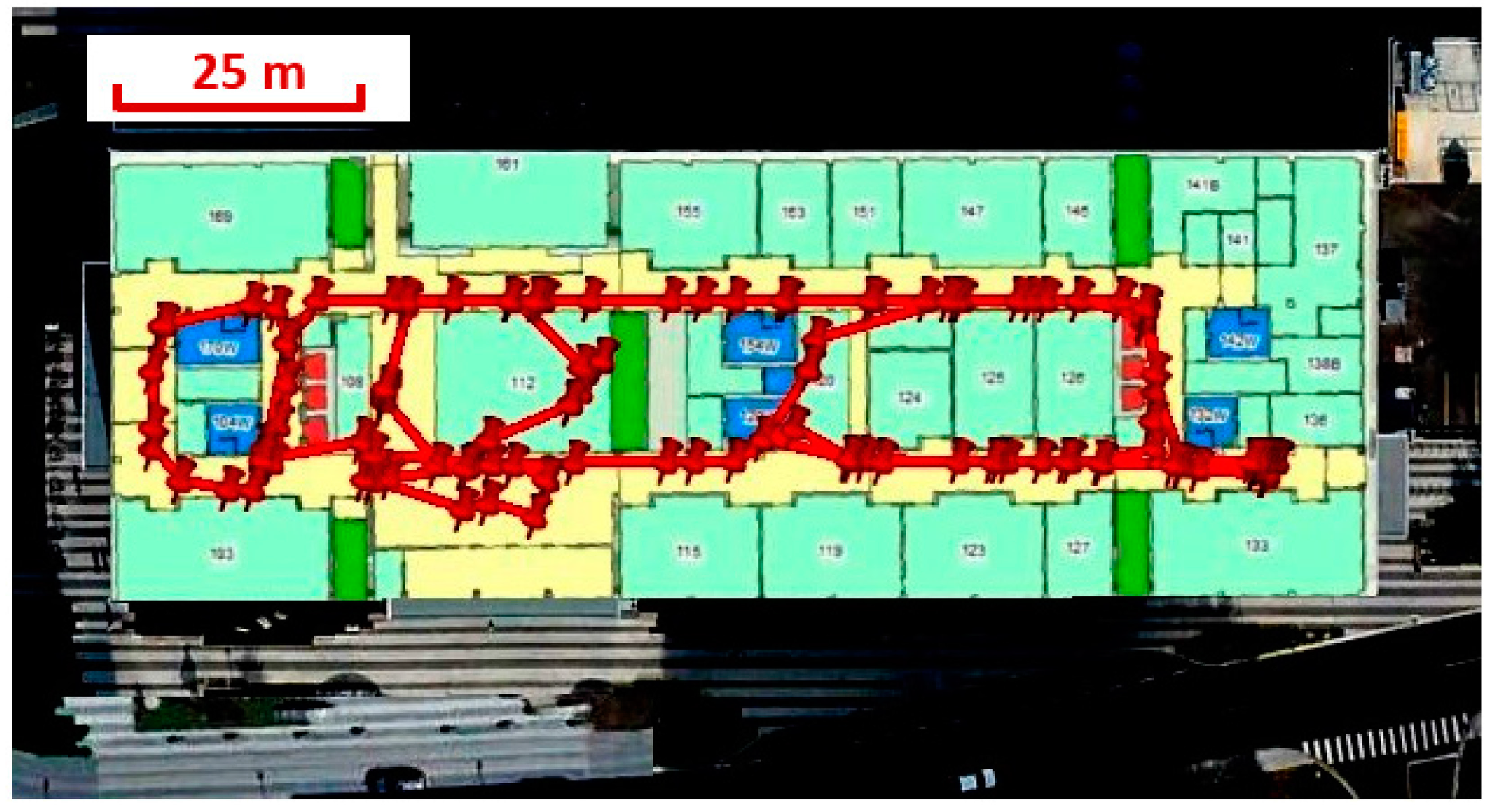
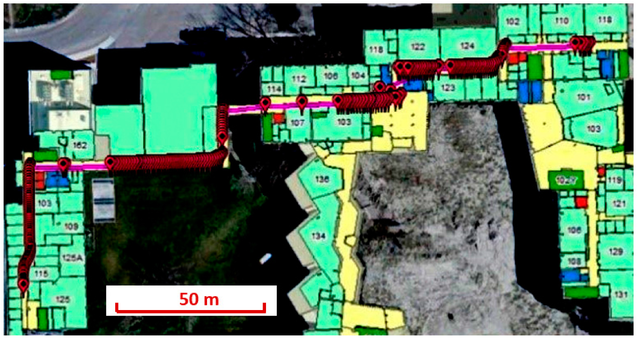
Figure 7 shows the trajectory for the positioning test, which was different from the training trajectories. The walking directions on the majority of the main corridors were also different from those on the training trajectories.

The threshold value for available WiFi RSS was set at Th_RSS = −85 dBm. The number k was set at 4 for the k-NN approach. The profile length for MM was 10 steps: The MM process began after the user had walked for 10 steps; after this, the magnetic fingerprints within the latest 10 steps were used for matching. The radius of the MM search space determined by the WiFi results was set at R = 15 m. The test results are shown in the next subsection.

Figure 7. Test trajectory at EEEL (with abundant WiFi and magnetic information).

Figure 7. Test trajectory at EEEL (with abundant WiFi and magnetic information).

3.1.3. EEEL Test Results

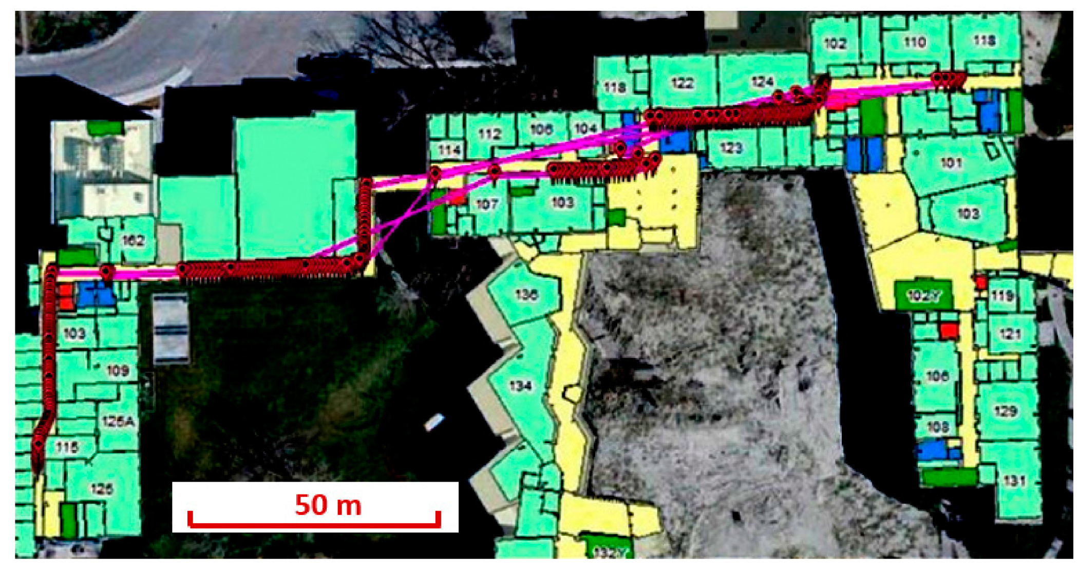
Navigation solutions with pedestrian dead-reckoning (PDR)-only, WiFi-only, MM-only, and WiFi-aided MM are shown in this subsection. We first trace the trajectory provided by each technology or combination. After this, statistical results are provided. The MM, WiFi, and WiFi-aided MM solutions are demonstrated in Figure 8, Figure 9 and Figure 10, respectively.

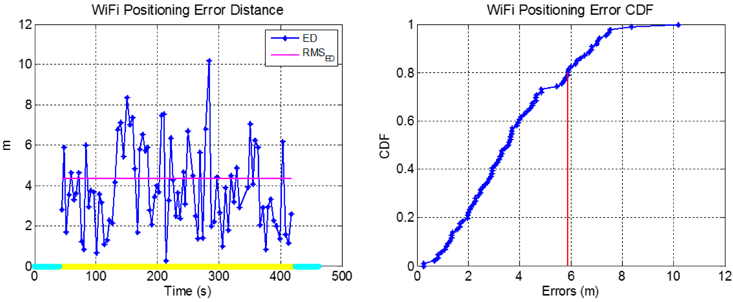
WiFi provided absolute positions with a low mismatch rate in this test. As there were abundant WiFi APs in EEEL, the ambiguity issue was not evident. However, the WiFi results had significant fluctuations. RSS fluctuation is an issue inherent to any technology based on RSS.

Compared with WiFi, the matched MM results were more accurate and had smaller fluctuations. Nevertheless, MM had a significantly larger mismatch rate. Thus, it is preferable to use other technologies to aid MM and detect the mismatches. Figure 10 shows that the majority of the mismatches in MM were eliminated by limiting the search space using the WiFi results.

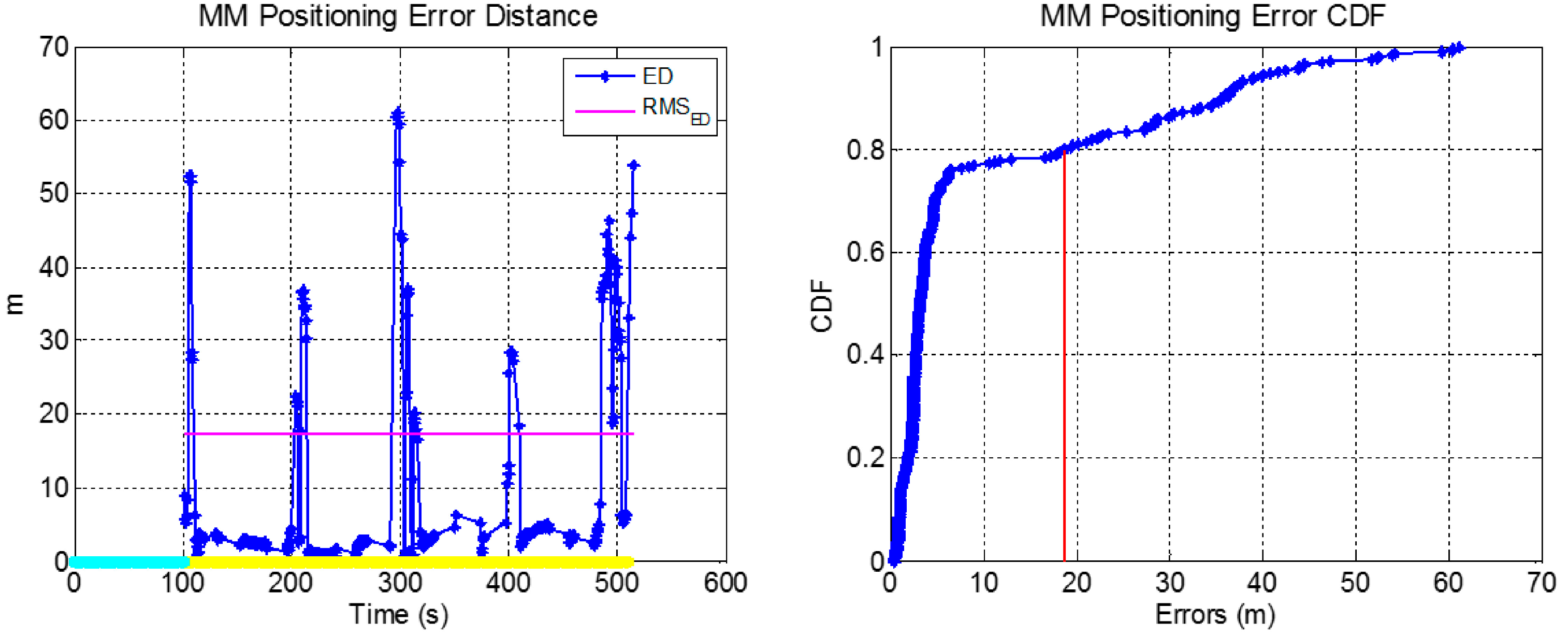
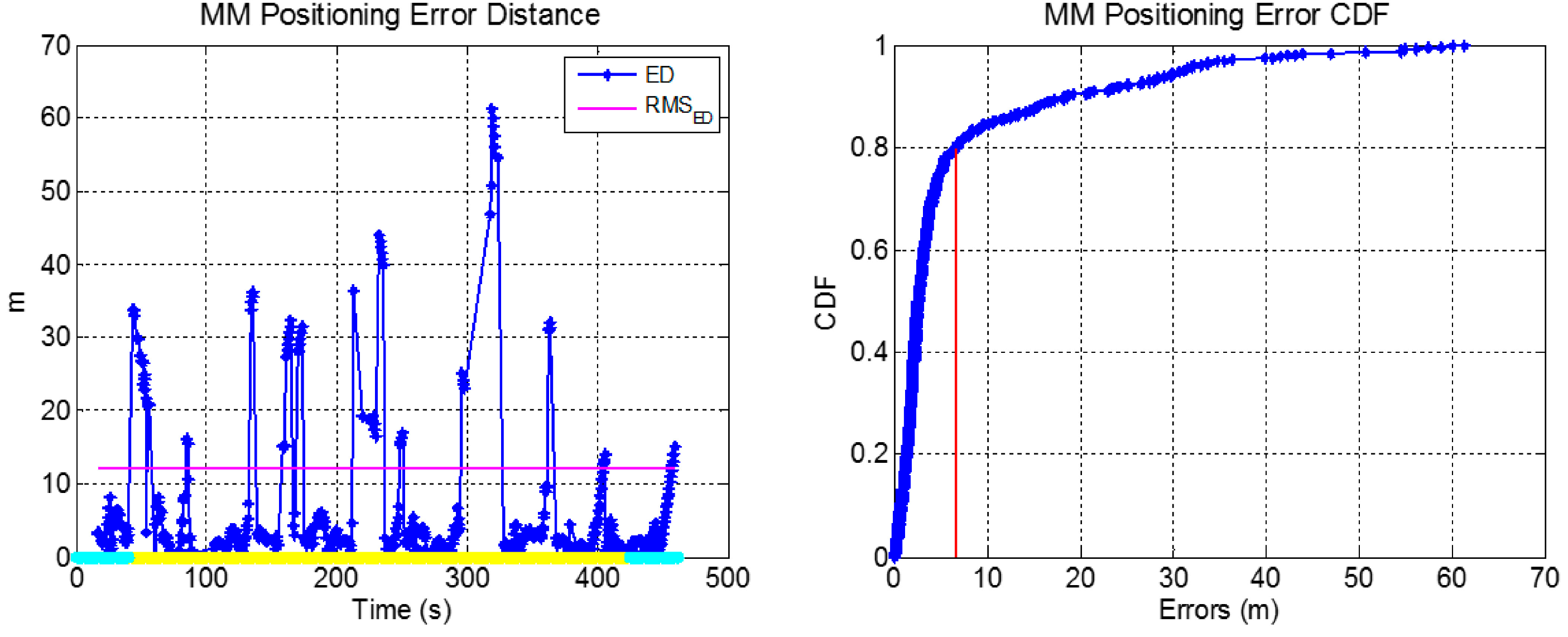
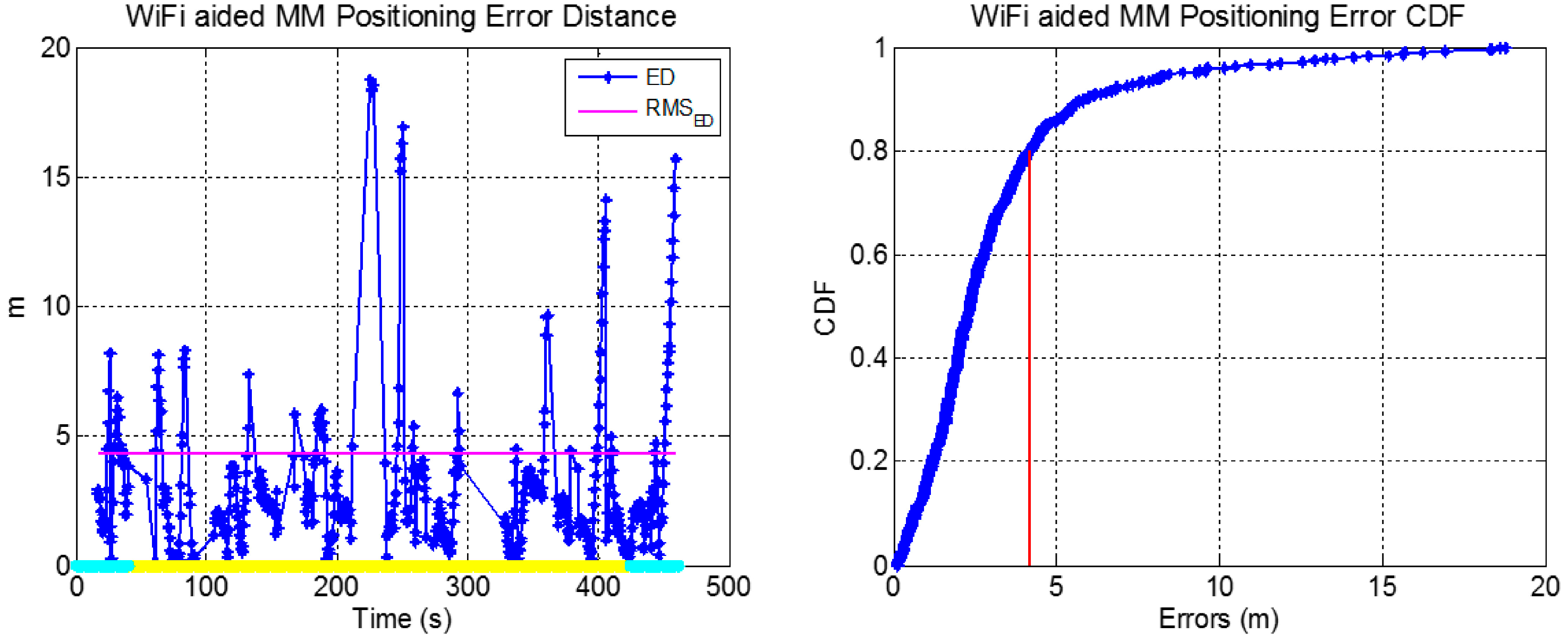
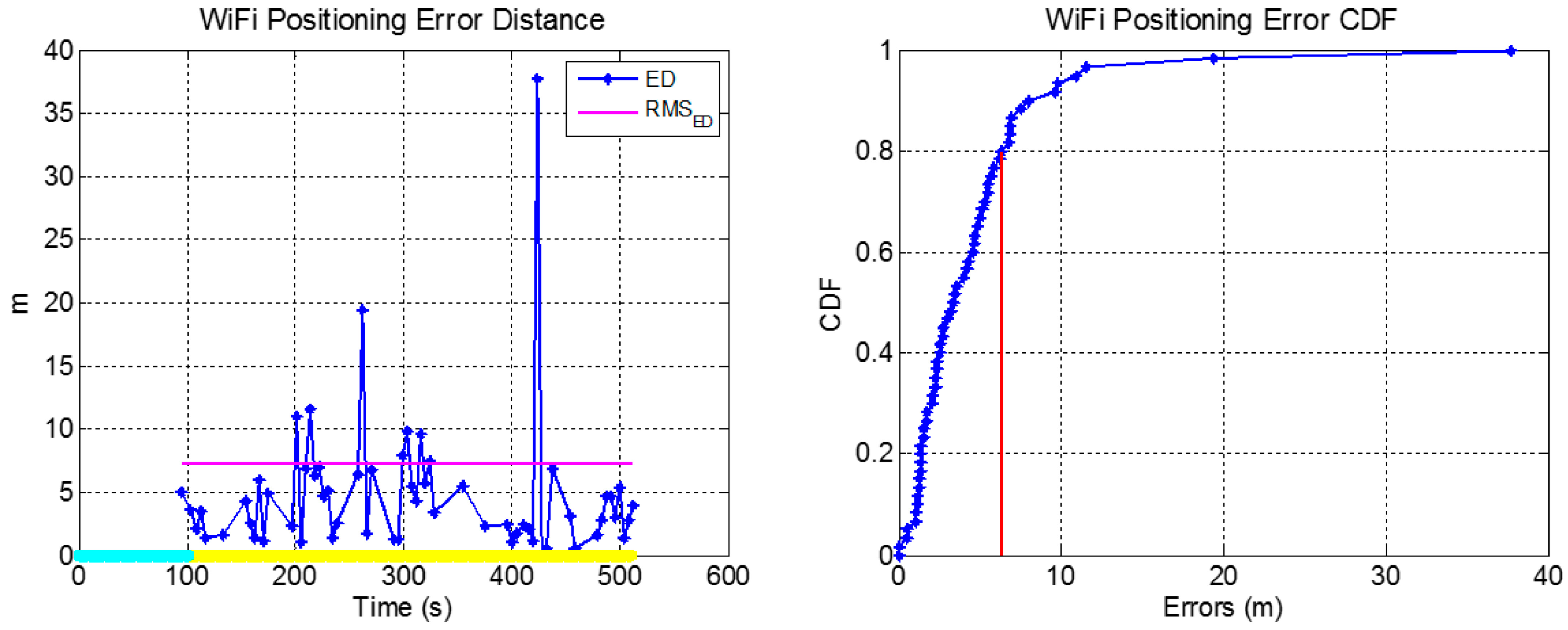
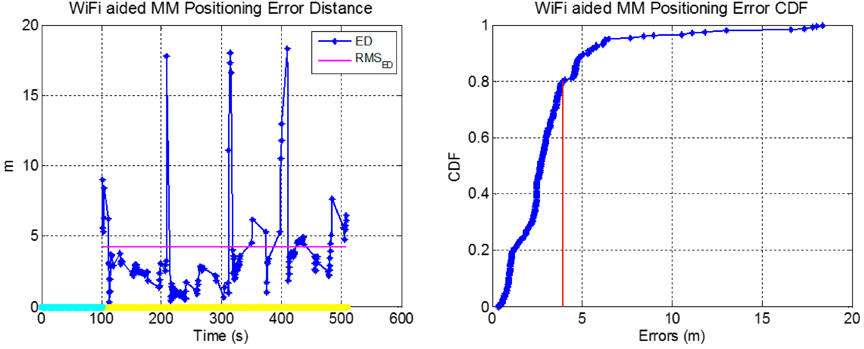
To further evaluate the positioning errors, the error distances (i.e., the distance between the estimated user position and the corresponding true position) were calculated. The true positions were obtained by using the floor plan to correct the PDR solution, which was similar to the work in the training phase. Figure 11, Figure 12 and Figure 13 demonstrate the position errors of MM, WiFi, and WiFi-aided MM, respectively. The left plot in each figure shows the time series of error distances. The root mean square (RMS) value of the error distances is also shown as a magenta line. The yellow and blue lines on the x-axis indicate indoors and outdoors, respectively. The right plot in each figure is the statistical error cumulative distribution function (CDF). The red line indicates the error within which the probability is 80%.

Figure 8. Magnetic matching (MM) result at EEEL.

Figure 8. Magnetic matching (MM) result at EEEL.

Figure 9. WiFi fingerprinting result at EEEL.

Figure 9. WiFi fingerprinting result at EEEL.

Figure 10. WiFi-aided MM result at EEEL.

Figure 10. WiFi-aided MM result at EEEL.

Figure 11. MM position errors at EEEL.

Figure 11. MM position errors at EEEL.

Figure 12. WiFi position errors at EEEL.

Figure 12. WiFi position errors at EEEL.

Figure 13. WiFi-aided MM position errors at EEEL.

Figure 13. WiFi-aided MM position errors at EEEL.

By using the WiFi solutions to limit the search space, the MM errors were reduced significantly. On several occasions, a sequence of MM results was more than 20 m away from the true positions. When aided by WiFi, these MM errors were controlled effectively. The max error reduced from more than 60 m to less than 20 m. Also, the 80% reduced from approximate 7 m to below 5 m.

Comparing with the WiFi-only results, the WiFi-aided MM results had a smaller 80% error. However, the max error of the WiFi-aided MM solution is larger than that in the WiFi results. The statistical values of navigation errors are shown in Table 1. The first column shows the used technologies, and Column 2–4 are the max, RMS values, and errors within which the probability is 80%.

Table 1. Statistical values of navigation errors at the Energy Environment Experiential Learning (EEEL).

Technique	Max (m)	RMS (m)	80% (m)
WiFi	10.2	4.3	5.8
MM	61.5	12.2	7.0
WiFi-aided MM	18.3	4.5	4.2

Table 1. Statistical values of navigation errors at the Energy Environment Experiential Learning (EEEL).

Technique	Max (m)	RMS (m)	80% (m)
WiFi	10.2	4.3	5.8
MM	61.5	12.2	7.0
WiFi-aided MM	18.3	4.5	4.2

The RMS of WiFi positioning errors was 4.3 m. This was a medium accuracy for WiFi with consumer portable devices and with walk-survey. 80% of MM errors were within 7.0 m, but the RMS was 12.2 m. This is because there were several large mismatches. The RMS of MM errors was reduced to 4.5 m when using WiFi results to limit the search space.

Although the 80% error of WiFi-aided MM was 1.6 m less than that of WiFi, both the max error and the error RMS of the former were larger. This might due to the fact that WiFi results were already accurate (with a RMS of 4.3 m) because there were over 10 WiFi signals in most of the tested area at EEEL. This outcome indicates the performance improvement by combing WiFi and MM depends on signal distributions of both magnetic intensity and WiFi RSS. The following tests at ENB show the performance of the WiFi-aided MM algorithm when there were less WiFi signals.

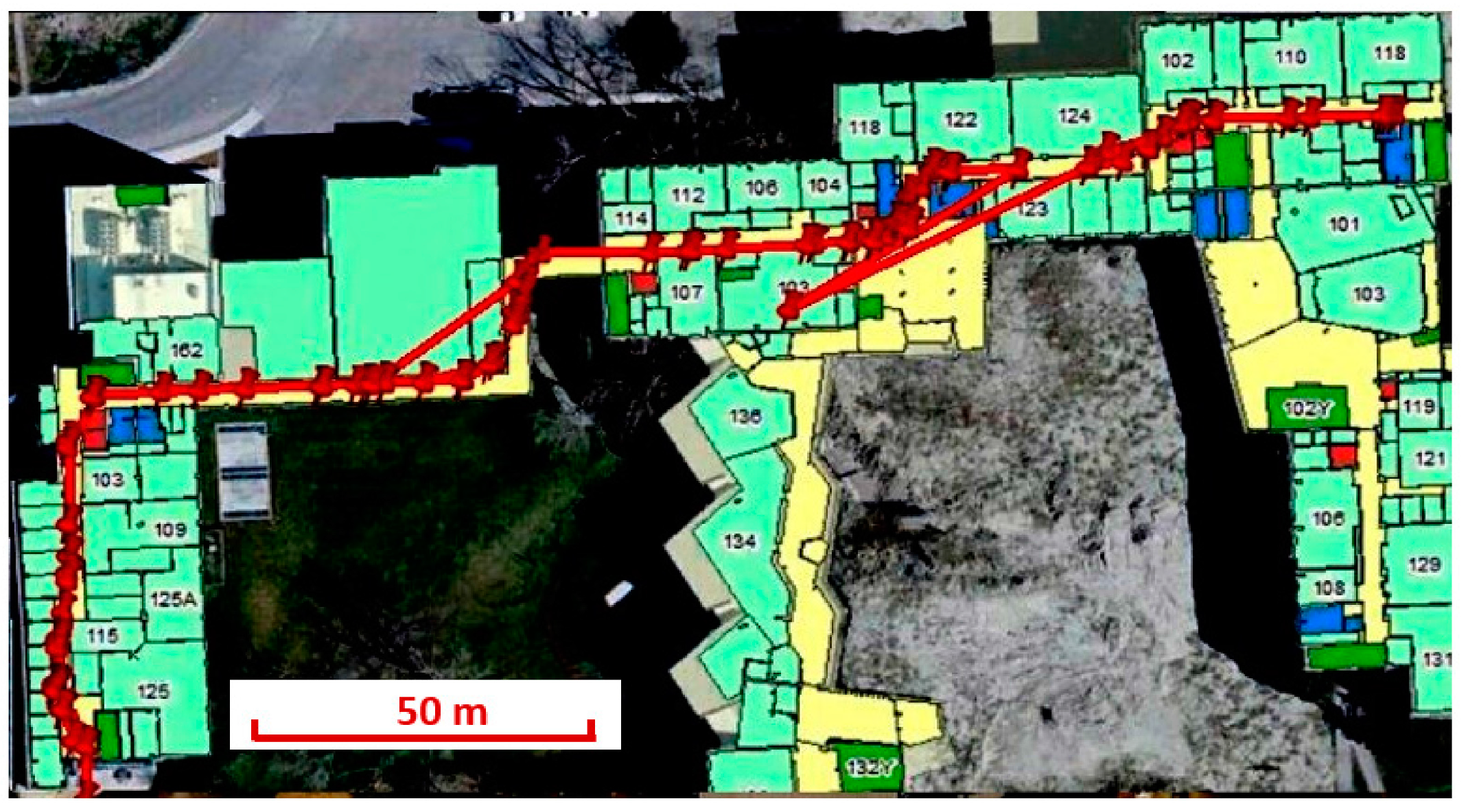
3.2. Tests at ENB

The corridors in ENB are narrow and straight, which are different from those in EEEL. The RSS and magnetic distributions on the tested trajectory are shown in Figure 14 and Figure 15, respectively. The average number of RSS was approximately seven, and the change of magnetic intensity was below 0.25 Gauss. There were less WiFi APs and less magnetic perturbations at ENB. Therefore, it was expected that the WiFi and MM accuracy would probably be lower than that at EEEL.

The MM, WiFi, and, WiFi-aided MM trajectories are demonstrated in Figure 16, Figure 17 and Figure 18, respectively.

Not only the MM results but also the WiFi results had several significant mismatches. This outcome met our expectation, as the WiFi signal distribution was poorer at ENB.

Figure 19, Figure 20 and Figure 21 demonstrate the position errors of MM, WiFi, and WiFi-aided MM, respectively. The left plot in each figure shows the time series of error distances. The root mean square (RMS) value of the error distances is also shown as a magenta line. The yellow and blue lines on the x-axis indicate indoors and outdoors. The right plot in each figure is the statistical error cumulative distribution function (CDF). The red line indicates the error within which the probability is 80%.

Figure 14. WiFi signal distribution at the Engineering building (ENB).

Figure 14. WiFi signal distribution at the Engineering building (ENB).

Figure 15. Magnetic distribution at ENB.

Figure 15. Magnetic distribution at ENB.

Figure 16. MM result at ENB.

Figure 16. MM result at ENB.

Figure 17. WiFi fingerprinting result at ENB.

Figure 17. WiFi fingerprinting result at ENB.

Figure 18. WiFi-aided MM result at ENB.

Figure 18. WiFi-aided MM result at ENB.

Figure 19. MM position errors at ENB.

Figure 19. MM position errors at ENB.

Figure 20. WiFi position errors at ENB.

Figure 20. WiFi position errors at ENB.

Figure 21. WiFi-aided MM position errors at ENB.

Figure 21. WiFi-aided MM position errors at ENB.

The RMS of MM errors was 16.6 m at ENB, which was larger than that at EEEL (12.2 m). Also, the WiFi errors were more significant and had a max error of 35 m. Even with such large WiFi errors, the WiFi-aided MM results had a much smaller max error and RMS than both the WiFi and MM results. The statistics of navigation errors are shown in Table 2.

Table 2. Statistical values of navigation errors at ENB.

Technique	Max (m)	RMS (m)	80% (m)
WiFi	37.8	7.2	6.3
MM	61.0	16.6	17.3
WiFi-aided MM	17.8	4.2	4.0

Table 2. Statistical values of navigation errors at ENB.

Technique	Max (m)	RMS (m)	80% (m)
WiFi	37.8	7.2	6.3
MM	61.0	16.6	17.3
WiFi-aided MM	17.8	4.2	4.0

In the ENB tests, MM provided the worst navigation solution with an RMS of 16.6 m. However, when aided by WiFi, the RMS reduced to 4.2 m. Therefore, although MM was not reliable, it could provide high accuracy when there was no mismatch. Therefore, it is feasible to combine MM with other technologies to provide accurate solutions. The key is to remove the MM mismatches using information from other technologies. When comparing the RMS value of the position errors for WiFi-aided MM with that for WiFi, an improvement of 41.6% was observed.

The WiFi and MM position errors at ENB (RMS 7.2 and 16.6 m, respectively) were more significant than those at EEEL (RMS 4.3 and 12.2 m, respectively). However, the position errors of WiFi-aided MM were similar for two buildings (RMS 4.5 m at EEEL and 4.2 m at ENB). This result indicates the potential of integrating WiFi and MM to provide more reliable navigation results, especially at the environments with poor WiFi RSS or magnetic intensity information. However, Figure 21 demonstrates that there were still several errors that were larger than 15 m. This may probably due to the accuracy limit of both WiFi and MM in a short time period. Therefore, PDR, which provided accurate short-term solutions but suffers from increasing drifts, may be an appropriate candidate to integrate with the WiFi-aided approach. This will be an important issue in our future research.

4. Conclusions

This paper presents a WiFi-aided magnetic matching (MM) navigation algorithm that maximizes the advantage and minimizes the disadvantage of WiFi and MM. By using WiFi to reduce the MM search space, this algorithm can significantly reduce the mismatching rate and computational load of MM. The algorithms were tested with smartphones in different indoor environments (i.e., Environment #1 with abundant WiFi APs and significant magnetic changes, and Environment #2 with less WiFi and magnetic information).

The WiFi and MM databases were generated simultaneously within half an hour using the walk-survey method. WiFi fingerprinting errors were not significant in Environment #1 (RMS 4.3 m and max 10.2 m) but significant in Environment #2 (RMS 7.2 m and max 37.8 m). In general, WiFi results had a low mismatch rate in both environments.

MM had significant mismatch rates. The RMS values of MM errors reached 12.2 m (Environment #1) and 16.6 m (Environment #2). However, when we used WiFi to limit the MM search space, the RMS reduced to below 4.5 m. Therefore, the key to obtaining accurate MM solutions is to remove the mismatches using information from other technologies.

WiFi-aided MM provided more reliable results than MM, which indicates the effectiveness of introducing the WiFi information. Comparing with WiFi-only results, the WiFi-aided MM solution was similar in Environment #1 but approximately 41.6% better in Environment #2. This outcome demonstrates that integrating WiFi and MM can also enhance the WiFi fingerprinting results in environments with poor WiFi signal distributions.

The proposed WiFi-aided magnetic matching algorithm uses off-the-shelf sensors available in consumer portable devices and existing WiFi infrastructure, which need no additional hardware cost or extra manpower cost. Future work will focus on introducing other technologies, such as PDR, to integrate with the WiFi-aided approach and provide continuous and reliable solutions.