1. Introduction
China has more than 70% of its land made up of mountains and hills, while the main agricultural terraces are located in southwest and southeast China. Therefore, agricultural terraces have become the most important agricultural land-use type and support the main agricultural production in these areas. Furthermore, it also plays an important role in reducing flood runoff, changing terrain slope and maintaining water, soil and conservation fertilizer.
However, due to Chinese agricultural policy and regional characteristics, most agricultural terraces in southwest and southeast China are farmed by smallholders, and have small sizes, scattered distributions, complex terrains and other characteristics. Such issues have increased difficulty in land use management and planting management of local governments, as well as regular cropping and planting area monitoring of smallholder farmers. Meanwhile, illegal land occupations, natural disasters, water and wind erosion are also causing a drastic decrease in agricultural terraces, and these further aggravate the soil erosion and endanger the smallholder production. Consequently, a light-weight and low cost dynamic monitoring of agricultural terraces has become a serious concern for smallholder production systems in China.
Agricultural terrace monitoring includes two major aspects: (i) crop monitoring and (ii) planting area monitoring. In this work, we mainly focus on the planting area monitoring, which generally depends on aerial remote sensing and image processing techniques. In parallel to the technological advances of aerial remote sensing, achievements in image processing have promoted the development of sophisticated algorithms using aerial images, such as the landform classification, which is one of the effective ways for dynamic monitoring of land-use changes. Traditional landform classification methods can be divided into non-supervised classification methods and supervised classification methods [
1]. Basically, non-supervised methods consist of manual classification methods and automated classification methods [
2]. Manual classification methods are relatively time-consuming and the results depend on subjective decisions of the interpreter and are, therefore, neither transparent nor reproducible [
3,
4]. Automated classification methods [
5,
6] make use of the unsupervised nature and automation of the change analysis process. However, they are unfavored by difficulties in identifying and labeling change trajectories [
7], and the lack of information on calibration of the ground [
7]. Artificial neural network (ANN) constitutes a key component of supervised classification methods [
8,
9]. It is a non-parametric method that is capable of estimating the properties of data based on the training samples. However, ANN suffers from the long training time, the sensitivity to the amount of training data used, as well as the applicability of ANN functions in the common image processing softwares [
7].
Subsequent to the landform classification, classified images can be adopted to monitor land use changes. Over the last few years, in order to analyze agricultural terraces, different and new technologies have been used. Satellite data of high spatial resolution and advanced image processing techniques, have opened up a new insight for mapping landscape features, such as terraces. This has given the opportunity for quantitative assessment of farming practices as an indicator in water pollution risk assessment [
10], soil erosion risk assessment [
11] and landslide boundary monitoring [
11,
12,
13,
14]. In addition, airborne LiDAR (light detection and ranging), which has been developed to collect and subsequently characterize vertically distributed attributes [
15], and the derived digital elevation model (DEM) [
16,
17,
18,
19,
20] or digital terrain model (DTM) [
12,
14] are becoming standard practices in spatial related areas. Recently, the use of unmanned aerial vehicle (UAV) for civil applications has emerged as an attractive and flexible option for the monitoring of various aspects of agriculture and environment [
21]. For example, Diaz-Varela et al. [
21] proposed an automatic identification of agricultural terraces through object-oriented analysis of high resolution digital surface models and multi-spectral images obtained from UAVs. Deffontaines et al. [
22] monitored the active inter-seismic shallow deformation of the Pingting terraces by using UAV high resolution topographic data combined with InSAR time series. Yang et al. [
23] proposed a multi-viewpoint remote sensing image registration method that provided an accurate mapping between different viewpoint images for ground change detections.
Compared with satellite and other aerial remote sensing, using small UAVs for agricultural terrace monitoring has a strong mobility, high efficiency, low cost and other advantages. However, the following issues still exist: (i) Due to the payload capacity, small UAVs usually can only carry a light-weight visible light camera, such as CCD or CMOS cameras that limit available image information while increasing difficulty in monitoring algorithms compared with using multi-spectral imaging. (ii) When collecting multi-temporal images for the same location (e.g., a planting area in terraces), the imaging perspective of small UAVs is often easily affected by wind speed/direction, complex terrain, battery capacity (e.g., flying distance), aircraft posture (pitch, roll, yaw), flying height and other human factors. These factors cause the captured scenes (i.e., the same location in a pair of multi-temporal images) to not be in the same coordinate system, while image geometric distortions, low image overlapping, brightness changes and color changes may also be produced in such multi-temporal images.
The above issues have led to the fact that multi-temporal images of the same scene captured by small UAVs may not be directly used to detect changes for dynamic agricultural terrace monitoring, and a reliable multi-temporal image registration, which can transform the images into one coordinate system, is necessary in order to be able to subsequently compare or integrate the data obtained from the multi-temporal images.
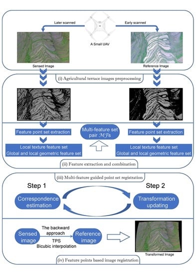
In this work, we focus on planting areas of agricultural terraces, and present a small UAV based multi-temporal image registration method for dynamic agricultural terrace monitoring. The major contributions of the proposed method includes: (i) the guided image filtering for agricultural terrace image preprocessing is first designed to enhance terrace ridges in multi-temporal images, (ii) the multi-feature descriptor is then applied to combine the texture feature and the geometric structure feature of terrace images for improving the description of feature points and rejecting outliers, (iii) the multi-feature guided model provides an accurate guiding for feature point set registration, and (iv) the feature points based image registration finally registers the terrace images accurately.
2. Methodology
The proposed small UAV based multi-temporal image registration method has four major sequential processes: (i) image preprocessing; (ii) feature extraction and combination; (iii) feature point set registration; and (iv) image registration. In this section, we first introduce the proposed method followed by analyzing the computational complexity and discussing the implementation details.
2.1. Guided Image Filtering Based Agricultural Terrace Image Preprocessing
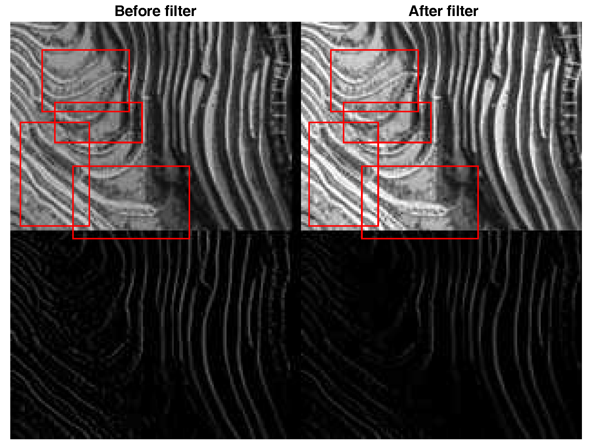
Given a gray agricultural terrace image with pixels and intensity = 0.3R + 0.59G + 0.11B from the colorized image captured by a small UAV. We first define a preprocessing method to strengthen the identifiability of terrace ridges in multi-temporal images, and then extract salient features of terrace images along the enhanced ridges in the second step. The main reason is that accuracy and validity of an image registration are not only controlled by the performance of feature point set registration, but also determined by the number and the distribution density of feature points, because of the image transformation constructed by abundant feature points.
In this work, the preprocessing method improves the contrast ratio between terraces and their ridges using the Guided Image Filtering (GIF) [
24]. In order to extract large and quality feature points from terrace ridges, we first adopt the GIF, which has the edge-preserving smoothing and the gradient preserving, to preprocess input images. The GIF employs a guidance image to construct a spatially variant kernel and is also related to the matting Laplacian matrix [
25].
Firstly, a linear translation-variant guided filtering process in a square window
centered at a pixel k is defined by:
where
i is a pixel index,
is the output image,
and
are two parameters of the minimal cost function
. Here,
g is the input image that is identical to the guidance image
,
and
are the mean and the variance of
in
,
is the number of pixels in
,
is a regularization parameter preventing
from being too large, and
is the mean of
g in
.
Secondly, we apply the linear model to all local windows in the entire image:
where
and
. An example of agricultural terrace image enhancement (
pixels) using GIF is given in
Figure 1.
An agricultural terrace is constructed by cropland and terrace ridges. Ridges can be considered as a salient feature that provides the features of geometric contours and surface textures for feature based terrace image registration. However, the flat color of terrace ridge is similar with croplands and detecting cropland and terrace ridges becomes difficult when crops are growing in the early stage. Thus, the extracted feature points along ridges are more helpful than points distributed on the cropland. Mathematically, the exponential function can change the density of the data distribution; therefore, we expand the gray value distribution of the common terrace via a natural exponential function formed as:
Finally, we can obtain the preprocessed gray agricultural terrace image with a high contrast ratio, smoothing edges, and prominent ridges. The preprocessing step gives an opportunity to extract quality features from these preprocessed terrace images.
2.2. Features Extraction and Combination
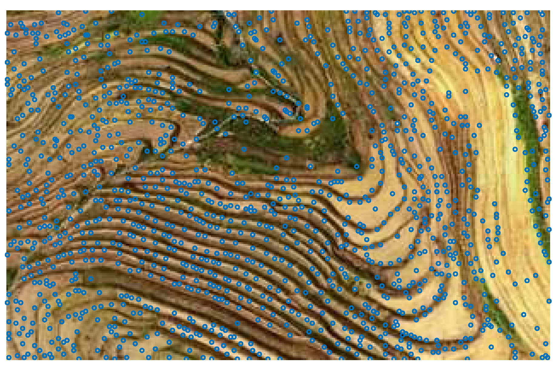
Feature points are selected by using the good-feature-to-track criterion [
26], similar to the Harris detector, based on the second moment matrix [
27]. The selection specifically maximizes the quality of tracking, and is therefore optimized by construction, as opposed to more ad hoc measures of texturedness. The selected feature point set
belongs with the geometric coordinate of a input agricultural terrace image pixel, where
. There is an example of feature points extraction from a preprocessed agricultural terrace image (
pixels) as shown in
Figure 2.
2.2.1. Local Texture Feature Descriptor
A local texture (LT) feature descriptor is designed to describe the texture features around each feature point according to the dominant rotated local binary patterns (DRLBP) proposed by Mehta [
28]. Given a gray image
with
pixels. The DRLBP operates in a local circular region by taking the difference of the central pixel with respect to its neighbors. It is defined as:
where
and
are the gray values of central pixel and its neighbor in image
, respectively,
and
are the geometric coordinate of the central pixel and its
lth neighbor. Note that
and
,
R is the radius of the circular neighborhood and
L is the number of the neighbors. The
indicates the modulus operator, and
. In this paper, the
are held in binary form. The DRLBP descriptor
of
is denoted by the DRLBP histogram
. The
operator circularly shifts the weights with respect to the dominant direction because of the weight term
depends on
D in the above definition. Therefore, the DRLBP is a rotation invariance and computationally efficient texture descriptor.
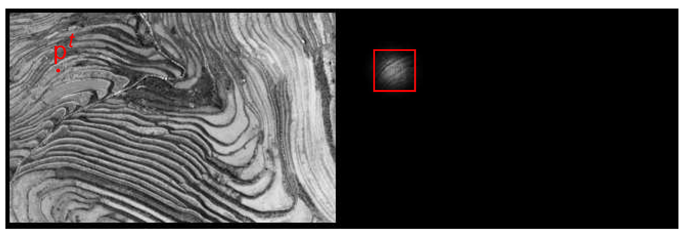
Before giving the LT for each feature point, the image is first weighted for each feature point based on its geometric coordinates, the weighting matrix for each point
is defined as:
where
is the geometric coordinate of the pixel
,
is the
tth point of
, and
is a parameter that controls the window size of LT.
is a
weighting matrix of the
tth feature point, and the
tth weighting gray image is obtained by:
where the weighting gray image
has the same size with the source gray image. Let
when
.
Figure 3 shows an example of weighting gray image.
We define the LT of the
tth feature point via DRLBP in the weighting gray image:
where
is a LT feature set with
T vectors both size of
.
2.2.2. Local Geometric Structure Feature Descriptor
A local geometric structure (LGS) feature is designed for each feature point in
by a local vector weighting method defined by:
where
is the index of
kth neighbor of
, and
K is the number of neighbors. The LGS descriptor employs the
K neighbors to give a LGS description for each feature point
but ignores outlier points. Hence, the value of
K and the weight term
play a crucial role for the performance of LGS. We use an outlier score to define the weight term of
:
where
is the variance of
, and the outlier score
is computed by the LT distance between
and the point that has the most similar LT feature with
as:
2.2.3. Multi-Feature Descriptor
Different types of feature descriptors have their own advantages and limitations. This motivates us to make the respective advantages of LT and LGS descriptors complementary to each other. The multi-feature (MF) is designed to combine the local texture information and the local geometric structure information for improving the identifiability of each feature point. However, a fixed falseness does no good for guiding point registration throughout the iterations. Thus, the MF descriptor is defined as:
where
and
are annealing parameters for the LGS and the LT features, respectively. The instantiation of Equation (11) is given in the implementation details section.
2.3. Multi-Feature Guided Point Set Registration Model
For feature based image registration, two sets of feature points are extracted from a pair of multi-temporal agricultural terrace images (i.e., a sensed image and a reference image), respectively. The extracted feature points contain a large number of outliers that limit the performance of current non-rigid point set registration algorithms [
29,
30,
31]. For this issue, a robust multi-feature guided model is designed—given two point sets
(i.e., the source point set) and
(i.e., the target point set) which are extracted from the sensed image and the reference image, respectively. The proposed point set registration model is first (i) to estimate correspondences between
and
by the proposed MF descriptor at each iteration, and then (ii) to update the location of
using a non-rigid transformation built by the recovered correspondences. The steps (i) and (ii) are iterated such that the
can gradually and continuously approach the target point set
, and finally match the exact corresponding points in
.
2.3.1. Correspondence Estimation
In the first step, the Gaussian mixture model (GMM) is applied to estimate correspondences by measuring the similarity of the MF between two point sets, and the correspondence estimation problem is considered as a GMM probability density estimation problem. Let the MF of
be the centroid of the
nth Gaussian component, and the MF of
be the
mth data. The GMM probability density function (PDF) is therefore obtained as:
where
with the equal isotropic covariances
of MF,
are non-negative equal quantity with
, which are called the priors of GMM.
is an additional uniform distribution with a weighting parameter
,
for outlier dealing.
Once we have the PDF of GMM that is guided by the similarity of MFs, we can estimate correspondence by the posterior probability of GMM via Bayes’ rule:
by which we obtain an one-to-many fuzzy correspondence matrix
guided by the similarity of MFs. Meanwhile, the corresponding target point set is obtained by:
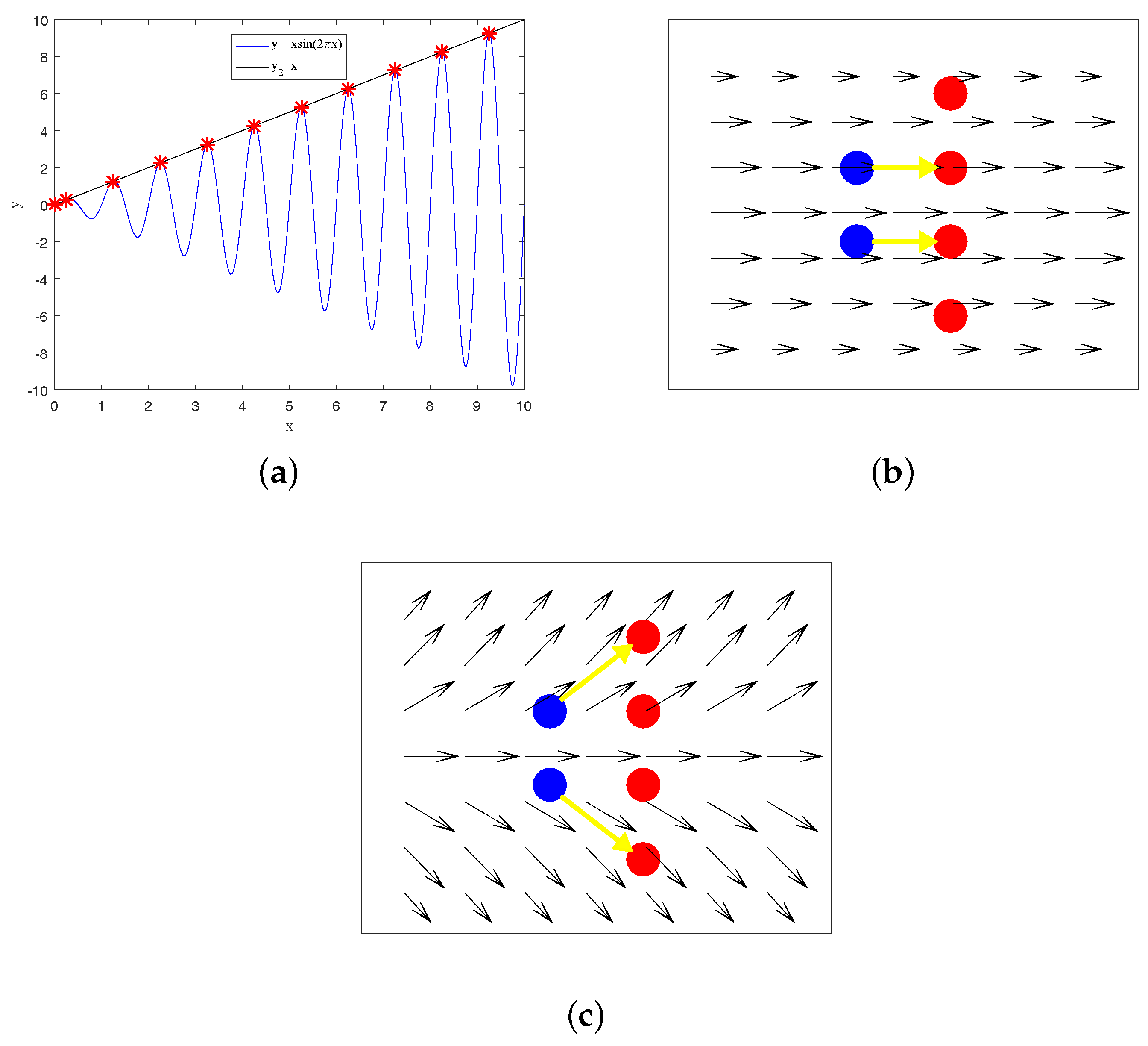
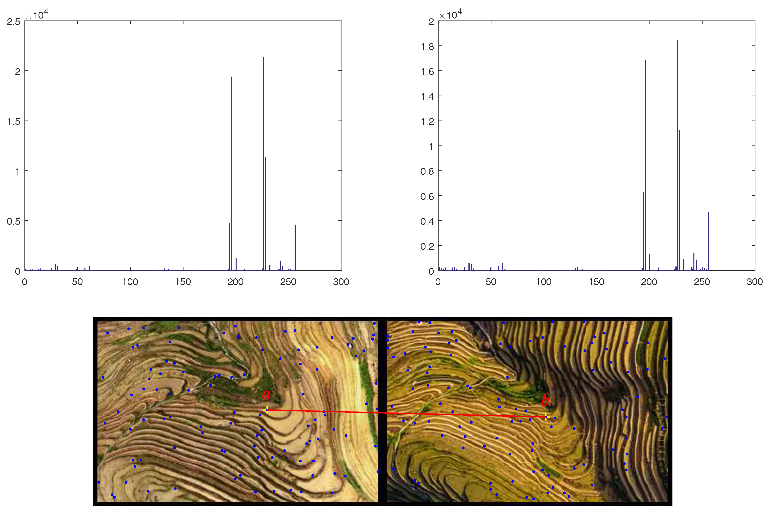
The proposed correspondence estimation method imitates the process of human practice, which measures the similarities of geometric structure feature and local texture feature. Generally, the process for humans to estimate the corresponding point of the source point
a in terrace image consists of two parts: (i) searching for a region in a reference image that has a similar geometrical location and structure compared to the region that surrounds source point
a, and (ii) finding a point within this region that has similar color features (LT in this paper) to the source point set. An example is shown in
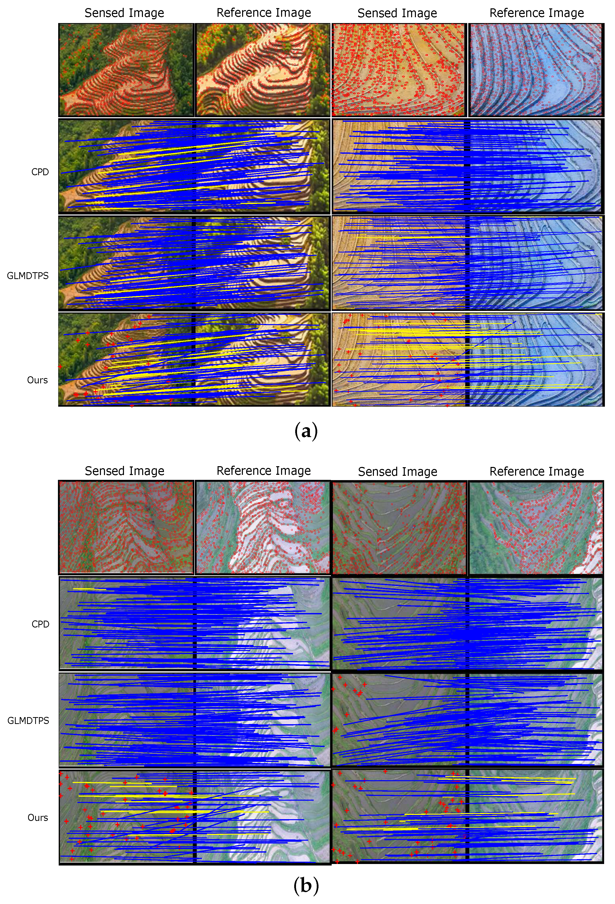
Figure 4, where only 100 feature points are shown for visual convenience. The two feature points
a and
b both have the similar pattern of LT histogram and the similar geometric feature.
2.3.2. Transformation Estimation
We model the non-rigid displacement function
f by requiring it to lie within a specific functional space, namely a vector-valued reproducing kernel Hilbert space (RKHS) [
32,
33]. The Gaussian kernel, which is in the form
and of size
, is chosen to be the associated kernel for the RKHS, where
is a constant to control the spatial smoothness. The function
f can be defined by:
Thus, the transformation estimation boils down to finding a finite parameter matrix W.
Before a direct parameter estimation, we first illustrate a rule by which a reliable transformation parameter is obtained in the estimation process.
Regularizing the transformation estimation process.
The adopted Tikhonov regularization framework [
34,
35,
36,
37] is one of the most common forms of regularization. It minimizes an energy function in an RKHS
to regularize a function
f, and can be written as:
In this paper, the function f is defined in Equation (15).
As shown in
Figure 5a, the regularized function (denoted by black line) is more reasonable than its non-regularized counterpart (denoted by blue curve). The transformation of an iterative registration method is such a procedure that slowly displaces the source point set so that the correspondence estimation is easier and more reliable. In other words, regularizing the transformation is necessary to accomplish the iterative registration.
Figure 5b,c indicate that the ill-posed problem will exist if the transformation is not regularized. Note that as the number of points increases, the increasing arbitrariness of the transformation will lead to more severe ill-posed problems.
The multi-feature guided fuzzy correspondence matrix
contains
probabilities, hence a reliable transformation will produce a larger expectation of probabilities. Therefore, the solution of transformation estimation is detected by maximizing a likelihood function that is formed as
, or equivalent to minimizing the negative log-likelihood function, which is formed as:
We use the maximizing expectation (M-step) of the expectation maximization (EM) algorithm [
29] to estimate the transformation. The idea of the EM algorithm is first to guess the values of parameters (“old” parameter values) via computing the posterior probability by Equation (13) (E-step), and then to find the “new” parameter values via minimizing the expectation of the complete negative log-likelihood function (M-step), which is formed as:
where
(with
only if
),
is the regularization of the transformation, and
is a weighting parameter controlling the strength of the regularization. Furthermore, with an initialized deterministic annealing parameter
, the parameter
W is obtained by
. The mathematical solution is detailed in
Section 2.5.
2.4. Feature Points Based Image Registration
Let and be the sensed and reference images, where the source point set and target point set are extracted from and , respectively. denotes the size of one image. Our goal is to obtain the transformed image .
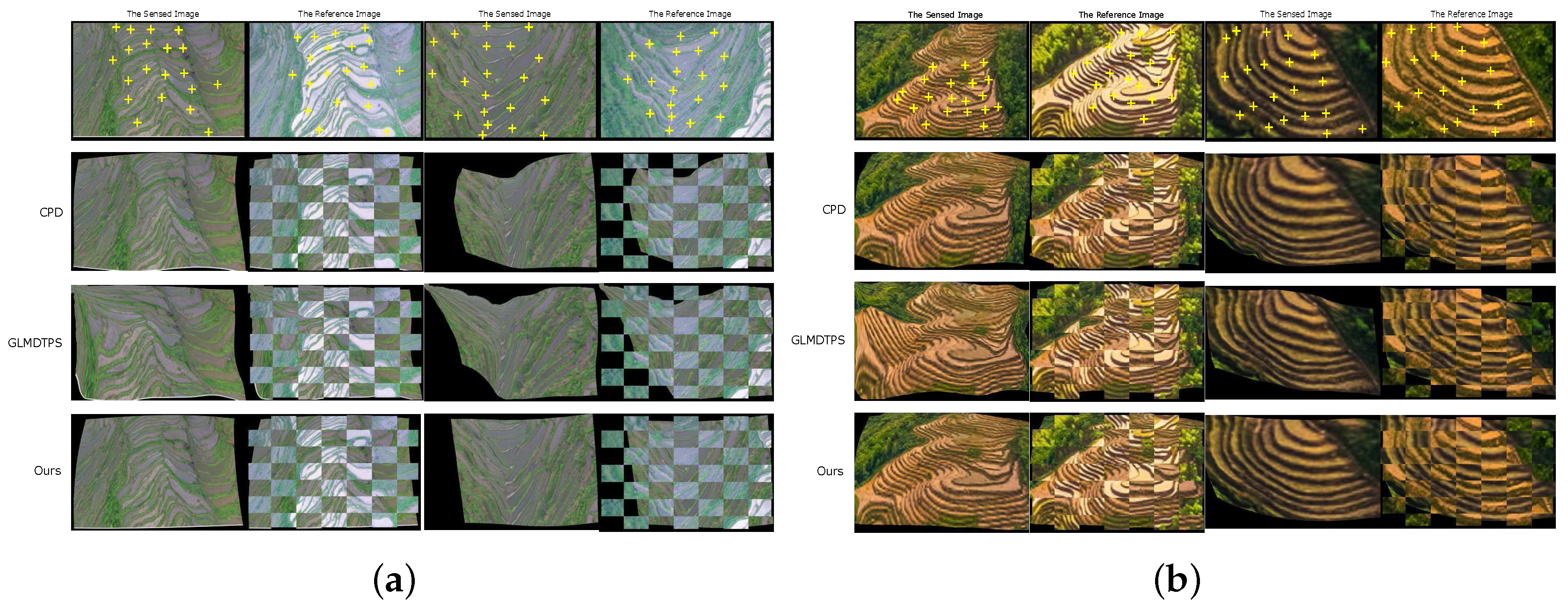
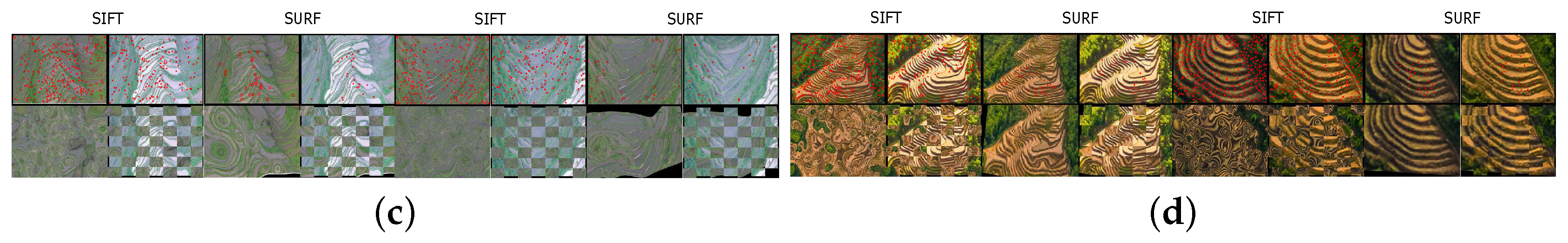
After the transformed source point set is obtained, a mapping function can be estimated based on the corresponding set that is constructed by and then the image registration can be realized. There are two types of mapping: (i) forward approach: directly transforming the sensed image using the mapping function, and (ii) backward approach: determining the transformed image from using the grid of the reference image and the inverse of the mapping. Due to the discretization and rounding, (i) is complicated to implement, as it can produce holes and/or overlaps in the output image, and we use the backward approach for image transformation.
We employ the TPS (thin plate spline) transformation model which obtained by:
where the TPS model
is of size
,
is a
matrix of zeros and
is the
matrix with the
nth denoting
, and the
TPS kernel
.
A regular grid
is obtained by a pixel-by-pixel indexing process on the reference image
, where
. Letting grid
be the source point set, and
the TPS transformation model, the transformed grid is obtained by first computing
then restoring the dimension of the grid to 2 by
, where the
kernel
,
is the
matrix with the
zth row denotes
and
denotes the
ith column of
. Let
be the grid obtained on
, we have
Finally, the transformed image is obtained by resampling intensities from the sensed image based on , setting the rest of pixels to black. Note that the bicubic interpolation is used to improve the smoothness of ; to be more precise, the intensities of each pixel in is determined by summing the weighted neighbor pixel intensities within a window.
2.5. Implementation Details
The instantiation of Equation (11) is impeded by LT descriptor
, which is constructed by a
dimension histogram. Actually, the goal of Equation (11) is to measure the distance of MFs, which means that instantiating
is equivalent to instantiating Equation (11). Analogically,
has two-dimensional terms and one
dimension term, hence, respectively instantiating
and
is equivalent to instantiating Equation (11). The distance of geometric and similarity of LT are denoted by Equations (22) and (23), in which the instantiation of
can be commonly realized by Euclidean distance computation. Furthermore, in general, a human similarity estimation of LT is to differentiate the pattern of the histogram, as we discussed in
Section 2.3.1. Therefore, we instantiate
by firstly normalizing each histogram in
, and then computing the quadratic distance sum of each dimension in the histogram, which is formed as:
where
denotes the
ith column of the histogram of
.
Once Equation (11) is instantiated, we can respectively rewrite Equations (13) and (18) by:
and
thus, we can complete the M-step of EM algorithm for implementing the agricultural terrace image registration. The matrix form of Equation (26) to simplify the derivative is written as:
where
denote trace operate,
,
is a column vector with all ones.
, where operator
is defined by
with
denoting a non-representational point set containing
I points,
is the index of the
kth neighbor of the
ith point,
K is the number of neighbors, and
is the weight of LGS defined by Equation (9). The partial derivative of Equation (27) with respect to the parameter
W is obtained by:
Setting Equation (28) to zero, the parameter
W is obtained by:
Parameter Setting
For evaluating image features, four groups of parameters—(i) R, the radius of the circular neighborhood in DRLBP; (ii) L, the number of the neighbors in DRLBP; (iii) , the window size controlled parameter in LT; and (iv) and , two annealing parameters for LGS and LT—are used. We set , , , and .
For registering extracted feature points, six parameters—(i)
, outlier weighting parameter; (ii)
, a constant to control the spatial smoothness; (iii)
, the equal isotropic covariances of MF; (iv)
W, the parameter of point set transformation; (v)
, the weighting parameter of regularization and (vi)
, the max number of iteration—are used. We set
,
and
, and initialize
W as a matrix with all zeros. Moreover,
and
are first initialized by
and
, then annealed as
and
respectively.
The pseudo-code of our feature points based agricultural terrace image registration is outlined in Algorithm 1.
| Algorithm 1: Local texture feature and geometric structure feature guided agricultural terrace image registration |
![Remotesensing 09 00904 i001]() |
2.6. Computational Complexity
The computational complexity of each part in our feature points based agricultural terrace image registration is as follows:
Image preprocessing:
time complexity: , space complexity: .
Feature extraction:
time complexity for feature points selection : , space complexity: ;
time complexity for computing LT: , space complexity: ;
time complexity for computing LGS: , space complexity: .
Point set registration:
time complexity for correspondence estimation: , space complexity: ;
time complexity for transformation estimation: , space complexity: .
Image registration:
time complexity: , space complexity: ,
where are the widths and heights of the source image and sensed image, respectively; are numbers of the feature points extracted from the source and sensed image. Overall, the time complexity of the proposed method is , and the space complexity is .


