
A Modified Dual-Baseline PolInSAR Method for Forest Height Estimation

 ,
,  and
and
Abstract
:
1. Introduction
2. Methods for Model-Based PolInSAR Forest Height Inversion
2.1. PolInSAR Coherence
2.2. RVoG Model
2.3. SBPI Method
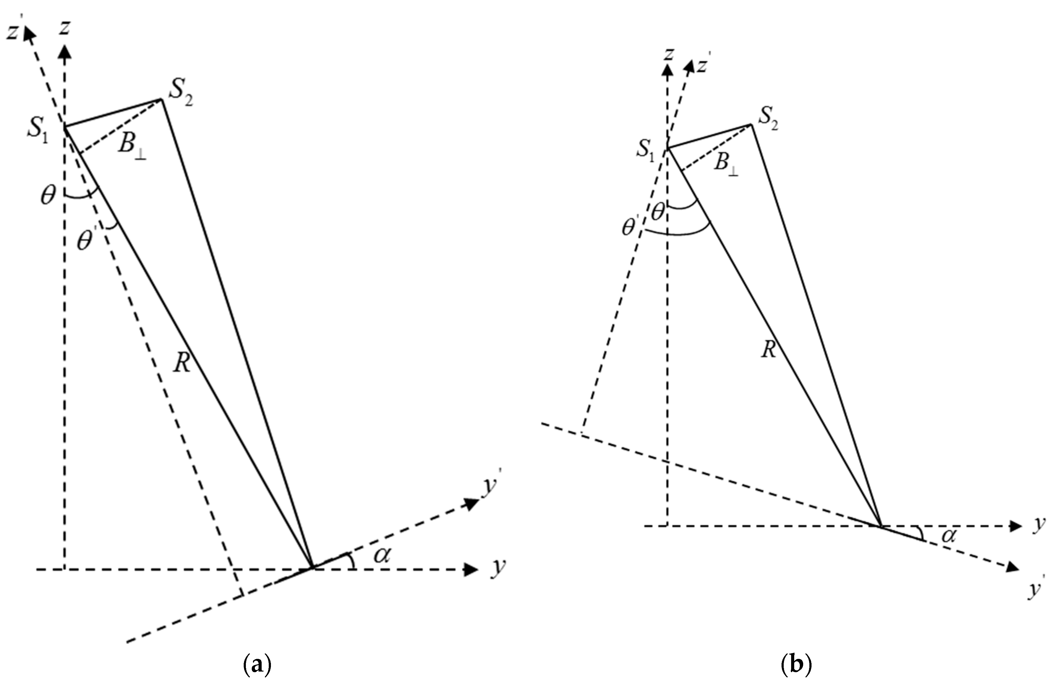
2.4. S-RVoG Model
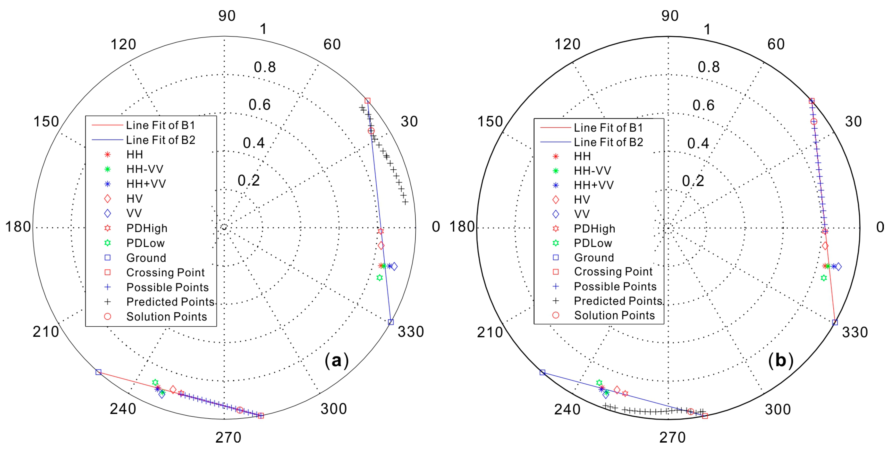
2.5. Cloude’s DBPI Method
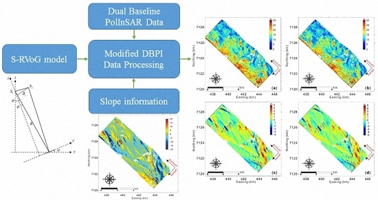
2.6. Modified DBPI Method
3. Test Site and PolInSAR Data Set Description
4. Results and Analysis
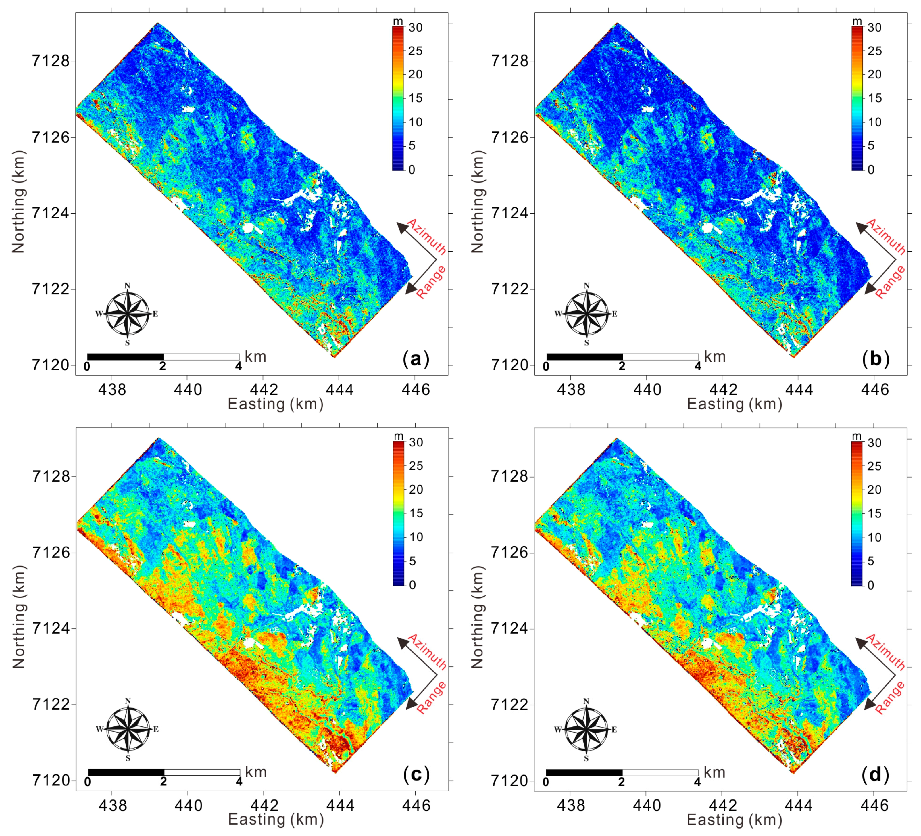
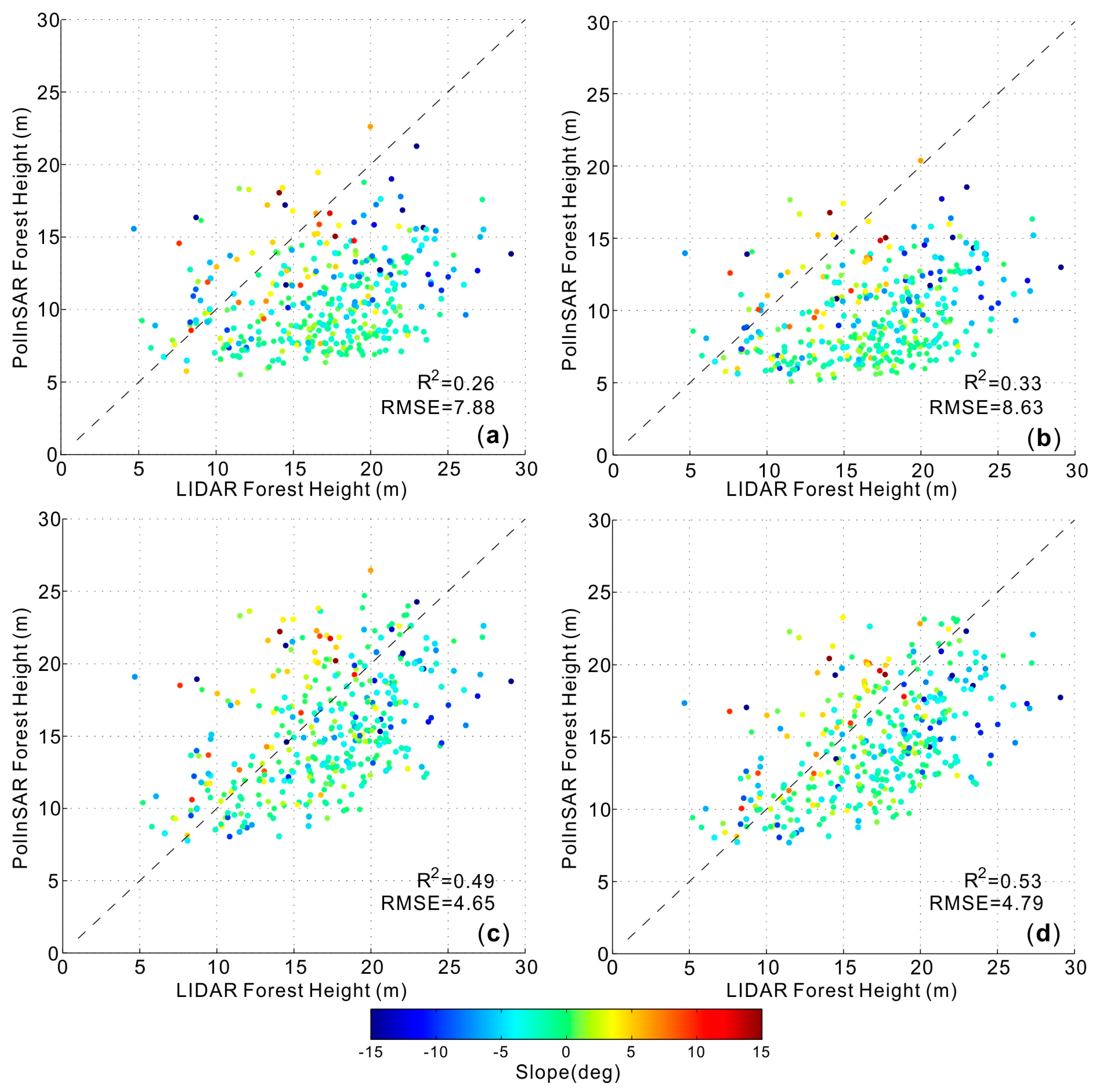
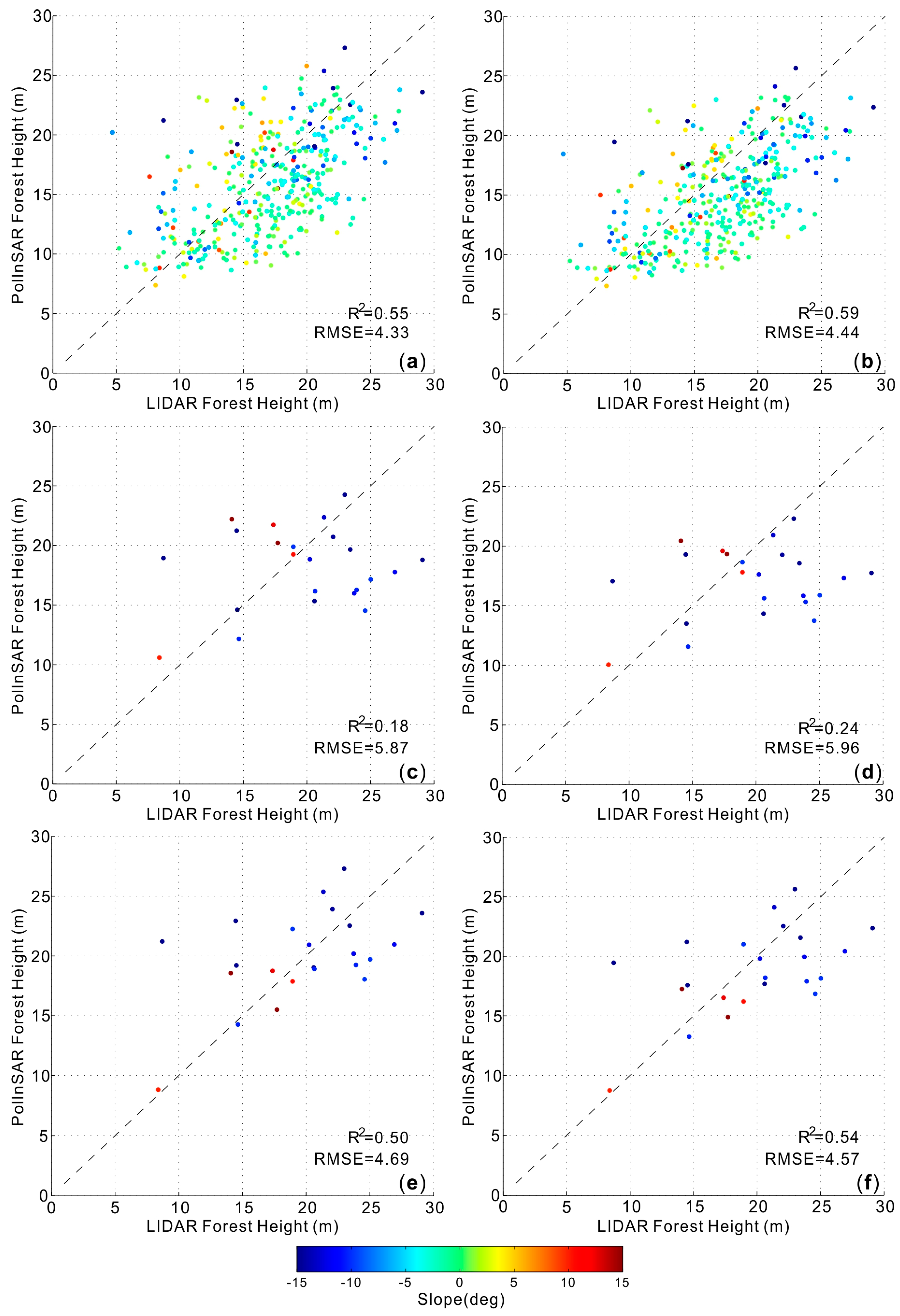
4.1. SBPI vs. Cloude’s DBPI
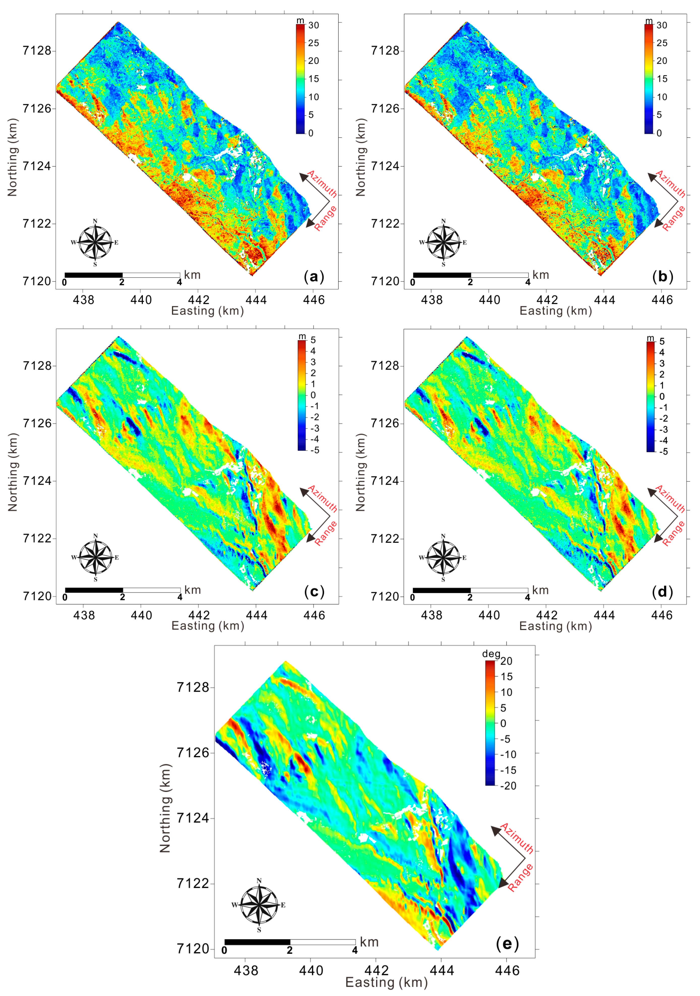
4.2. Cloude’s DBPI vs. Modified DBPI
5. Discussion
6. Conclusions
Acknowledgments
Author Contributions
Conflicts of Interest
References
- Pan, Y.; Birdsey, R.A.; Fang, J.; Houghton, R.; Kauppi, P.E.; Kurz, W.A.; Phillips, O.L.; Shvidenko, A.; Lewis, S.L.; Canadell, J.G.; et al. A Large and Persistent Carbon Sink in the World’s Forests. Science 2011, 333, 988–993. [Google Scholar] [CrossRef] [PubMed]
- Houghton, R.A.; Hall, F.; Goetz, S.J. Importance of biomass in the global carbon cycle. J. Geophys. Res. Biogeosci. 2009, 114, 1–13. [Google Scholar] [CrossRef]
- Cloude, S.R. Polarisation: Applications in Remote Sensing; Oxford University Press: New York, NY, USA, 2009. [Google Scholar]
- Treuhaft, R.N.; Madsen, S.N.; Moghaddam, M.; van Zyl, J.J. Vegetation characteristics and underlying topography from interferometric data. Radio Sci. 1996, 31, 1449–1495. [Google Scholar] [CrossRef]
- Treuhaft, R.N.; Siqueira, P.R. Vertical structure of vegetated land surfaces from interferometric and polarimetric data. Radio Sci. 2000, 35, 141–177. [Google Scholar] [CrossRef]
- Cloude, S.R.; Papathanassiou, K.P. Polarimetric SAR Interferometry. IEEE Trans. Geosci. Remote Sens. 1998, 36, 1551–1565. [Google Scholar] [CrossRef]
- Papathanassiou, K.P.; Cloude, S.R. Single-baseline polarimetric SAR interferometry. IEEE Trans. Geosci. Remote Sens. 2001, 39, 2352–2363. [Google Scholar] [CrossRef]
- Cloude, S.R.; Papathanassiou, K.P. Three-stage inversion process for polarimetric SAR interferometry. IEE Proc. Radar Sonar Navig. 2003, 150, 125–134. [Google Scholar] [CrossRef]
- Praks, J.; Kugler, F.; Papathanassiou, K.P.; Hawsek, I.; Hallikainen, M. Height estimation of boreal forest: Interferometric model-based inversion at L- and X-band versus HUTSCAT profiling scatterometer. IEEE Geosci. Remote Sens. Lett. 2007, 4, 466–470. [Google Scholar] [CrossRef]
- Garestier, F.; Dubois-Fernandez, P.C.; Champion, I. Forest Height Inversion Using High-Resolution P-Band Pol-InSAR Data. IEEE Trans. Geosci. Remote Sens. 2008, 46, 3544–3559. [Google Scholar] [CrossRef]
- Garestier, F.; Dubois-Fernandez, P.C.; Papathanassiou, K.P. Pine forest height inversion using single-pass X-band PolInSAR data. IEEE Trans. Geosci. Remote Sens. 2008, 46, 59–68. [Google Scholar] [CrossRef] [Green Version]
- Hajnsek, I.; Kugler, F.; Lee, S.K.; Papathanassiou, K.P. Tropical-Forest-Parameter Estimation by Means of Pol-InSAR: The INDREX-II Campaign. IEEE Trans. Geosci. Remote Sens. 2009, 47, 481–493. [Google Scholar] [CrossRef] [Green Version]
- Neumann, M.; Ferro-Famil, L.; Reigber, A. Estimation of forest structure, ground, and canopy layer characteristics from multibaseline polarimetric interferometric SAR data. IEEE Trans. Geosci. Remote Sens. 2010, 48, 1086–1104. [Google Scholar] [CrossRef] [Green Version]
- Garestier, F.; Dubois-Fernandez, P.; Champion, I.; Le Toan, T. Pine forest investigation using high resolution P-band Pol-InSAR data. Remote Sens. Environ. 2011, 115, 2897–2905. [Google Scholar] [CrossRef]
- Li, Z.; Guo, M.; Wang, Z.Q.; Zhao, L.F. Forest-height inversion using repeat-pass spaceborne polInSAR data. Sci. China Earth Sci. 2014, 57, 1314–1324. [Google Scholar] [CrossRef]
- Kugler, F.; Schulze, D.; Hajnsek, I.; Pretzsch, H.; Papathanassiou, K.P. TanDEM-X Pol-InSAR Performance for Forest Height Estimation. IEEE Trans. Geosci. Remote Sens. 2014, 52, 6404–6422. [Google Scholar] [CrossRef]
- Xie, Q.; Zhu, J.; Wang, C.; Fu, H. Boreal forest height inversion using E-SAR PolInSAR data based coherence optimization methods and three-stage algorithm. In Proceedings of the 3th International Workshop on Earth Observation and Remote Sensing Applications, Changsha, China, 11–14 June 2014; pp. 145–150. [Google Scholar]
- Fu, H.; Wang, C.; Zhu, J.; Xie, Q.; Zhao, R. Inversion of vegetation height from PolInSAR using complex least squares adjustment method. Sci. China Earth Sci. 2015, 58, 1018–1031. [Google Scholar] [CrossRef]
- Fu, H.; Wang, C.; Zhu, J.; Xie, Q.; Zhang, B. Estimation of Pine Forest Height and Underlying DEM Using Multi-Baseline P-Band PolInSAR Data. Remote Sens. 2016, 8, 820. [Google Scholar] [CrossRef]
- Wang, C.; Wang, L.; Fu, H.; Xie, Q.; Zhu, J. The Impact of Forest Density on Forest Height Inversion Modeling from Polarimetric InSAR Data. Remote Sens. 2016, 8, 291. [Google Scholar] [CrossRef]
- Garestier, F.; Le Toan, T. Forest modeling for height inversion using single-baseline InSAR/Pol-InSAR data. IEEE Trans. Geosci. Remote Sens. 2010, 48, 1528–1539. [Google Scholar] [CrossRef]
- Lavalle, M.; Simard, M.; Hensley, S. A temporal decorrelation model for polarimetric radar interferometers. IEEE Trans. Geosci. Remote Sens. 2012, 50, 2880–2888. [Google Scholar] [CrossRef]
- Lei, Y.; Siqueira, P.; Treuhaft, R. A physical scattering model of repeat-pass InSAR correlation for vegetation. Waves Random Complex Media 2017, 27, 129–152. [Google Scholar] [CrossRef]
- Lu, H.; Suo, Z.; Guo, R.; Bao, Z. S-RVoG model for forest parameters inversion over underlying topography. Electron. Lett. 2013, 49, 618–620. [Google Scholar] [CrossRef]
- Kugler, F.; Lee, S.K.; Hajnsek, I.; Papathanassiou, K.P. Forest Height Estimation by Means of Pol-InSAR Data Inversion: The Role of the Vertical Wavenumber. IEEE Trans. Geosci. Remote Sens. 2015, 53, 5294–5311. [Google Scholar] [CrossRef]
- Xie, Q.; Zhu, J.; Wang, C.; Fu, H. Forest height inversion by combining S-RVOG model with terrain factor and PD coherence optimization. Acta Geod. Cartogr. Sin. 2015, 6, 686–693. [Google Scholar]
- Xie, Q.; Wang, C.; Zhu, J.; Fu, H.; Wang, C. Improvement of forest height retrieval by integration of dualbaseline PolInSAR data and external DEM data. In Proceedings of the 2015 International Workshop on Image and Data Fusion (IWIDF 2015), Kona, HI, USA, 21–23 July 2015; pp. 185–189. [Google Scholar]
- Cloude, S.R. Robust parameter estimation using dual baseline polarimetric SAR interferometry. In Proceedings of the IEEE International Geoscience and Remote Sensing Symposium (IGARSS2002), Toronto, ON, Canada, 24–28 June 2002; pp. 838–840. [Google Scholar]
- Lavalle, M.; Khun, K. Three-baseline InSAR estimation of forest height. IEEE Geosci. Remote Sens. Lett. 2014, 11, 1737–1741. [Google Scholar] [CrossRef]
- Kugler, F.; Lee, S.; Papathanassiou, K.P. Estimation of forest vertical structure parameter by means of multi-baseline Pol-InSAR. In Proceedings of the IEEE International Geoscience and Remote Sensing Symposium, Cape Town, South Africa, 12–17 July 2009; pp. III-721–III-724. [Google Scholar]
- Lee, S.K.; Kugler, F.; Papathanassiou, K.P.; Hajnsek, I. Multibaseline polarimetric SAR interferometry forest height inversion approaches. In Proceedings of the 5th International Workshop on Science and Applications of SAR Polarmetry and Polarimetric interferometry (POLINSAR2011), Frascati, Italy, 24–28 January 2011; pp. 1–7. [Google Scholar]
- Bamler, R.; Hartl, P. Synthetic aperture radar interferometry. Inverse Probl. 1998, 14, R1–R54. [Google Scholar] [CrossRef]
- Freeman, A.; Durden, S.L. A three-component scattering model for polarimetric SAR data. IEEE Trans. Geosci. Remote Sens. 1998, 36, 963–973. [Google Scholar] [CrossRef]
- Xie, Q.; Ballester-Berman, J.D.; Lopez-Sanchez, J.M.; Zhu, J.; Wang, C. Quantitative analysis of polarimetric model-based decomposition methods. Remote Sens. 2016, 8, 977. [Google Scholar] [CrossRef]
- Xie, Q.; Ballester-Berman, J.D.; Lopez-Sanchez, J.M.; Zhu, J.; Wang, C. On the use of generalized volume scattering models for the improvement of general polarimetric model-based decomposition. Remote Sens. 2017, 9, 117. [Google Scholar] [CrossRef]
- Ballester-Berman, J.D.; Lopez-Sanchez, J.M. Applying the Freeman-Durden Decomposition Concept to Polarimetric SAR Interferometry. IEEE Trans. Geosci. Remote Sens. 2010, 48, 466–479. [Google Scholar] [CrossRef]
- Fu, H.; Zhu, J.; Wang, C.; Wang, H.; Zhao, R. Underlying Topography Estimation over Forest Areas Using High-Resolution P-Band Single-Baseline PolInSAR Data. Remote Sens. 2017, 9, 363. [Google Scholar] [CrossRef]
- Zhu, J.; Xie, Q.; Zuo, T.; Wang, C.; Xie, J. Criterion of complex least squares adjustment and its application in tree height inversion with PolInSAR data. Acta Geod. Cartogr. Sin. 2014, 43, 45–51. [Google Scholar]
- Fu, H.; Zhu, J.; Wang, C.; Xie, Q.; Zhao, R. Polarimetric SAR interferometry vegetation height inversion method of complex least squares adjustment. Acta Geod. Cartogr. Sin. 2014, 43, 1061–1607. [Google Scholar]
- Fu, W.; Guo, H.; Li, X.; Tian, B.; Sun, Z. Extended three-Stage polarimetric SAR interferometry algorithm by dual-polarization Data. IEEE Trans. Geosci. Remote Sens. 2016, 54, 2792–2802. [Google Scholar]
- Tabb, M.; Orrey, J.; Flynn, T.; Carande, R. Phase diversity: A decomposition for vegetation parameter estimation using polarimetric SAR interferometry. In Proceedings of the 4th European Synthetic Aperture Radar Conference (EUSAR2002), Cologne, Germany, 4–6 June 2002; pp. 721–724. [Google Scholar]
- Lavalle, M.; Solimini, D.; Pottier, E.; Desnos, Y.-L. Forest parameters inversion using Polarimetric and Interferometric SAR data. In Proceedings of the IEEE International Geoscience and Remote Sensing Symposium, Cape Town, South Africa, 12–17 July 2009; pp. IV-29–IV-132. [Google Scholar]
- Roueff, A.; Arnaubec, A.; Dubois-Fernandez, P.C.; Réfrégier, P. Cramer-Rao lower bound analysis of vegetation height estimation with random volume over ground model and polarimetric SAR interferometry. IEEE Geosci. Remote Sens. Lett. 2011, 8, 1115–1119. [Google Scholar] [CrossRef]
- DLR Microwaves and Radar Institute; Swedish Defense Research Agency; Politecnico di Milano POLIMI. BIOSAR 2008: Data Acquisition and Processing Report. 2008. Available online: https://earth.esa.int/c/document_library/get_file?folderId=21020&name=DLFE-903.pdf (accessed on 1 July 2017).
- Garestier, F.; Le Toan, T. Estimation of the backscatter vertical profile of a pine forest using single baseline P-band (Pol-)InSAR data. IEEE Trans. Geosci. Remote Sens. 2010, 48, 3340–3348. [Google Scholar] [CrossRef]
- Flynn, T.; Tabb, M.; Carande, R. Coherence region shape estimation for vegetation parameter estimation in POLINSAR. In Proceedings of the IEEE International Geoscience and Remote Sensing Symposium, Toronto, ON, Canada, 24–28 June 2002; pp. 2596–2598. [Google Scholar]
- Ferro-Famil, L.; Neumann, M.; Huang, Y. Multi-baseline POL-InSAR statistical techniques for the characterization of distributed media. In Proceedings of the IEEE International Geoscience and Remote Sensing Symposium, Cape Town, South Africa, 12–17 July 2009; pp. III-971–III-974. [Google Scholar]
- Ballester-Berman, J.D.; Lopez-Sanchez, J.M.; Fortuny-Guasch, J. Retrieval of biophysical parameters of agricultural crops using polarimetric SAR interferometry. IEEE Trans. Geosci. Remote Sens. 2005, 43, 683–694. [Google Scholar] [CrossRef]
- Lopez-Sanchez, J.M.; Ballester-Berman, J.D.; Marquez-Moreno, Y. Model limitations and parameter-estimation methods for agricultural applications of polarimetrie SAR interferometry. IEEE Trans. Geosci. Remote Sens. 2007, 45, 3481–3493. [Google Scholar] [CrossRef]


| Image | Temporal Baseline (min) | Baseline (m) | Kz Interval |
|---|---|---|---|
| 1 | 0 | 0 | master |
| 2 | 53 | 24 | 0.024–0.135 |
| 3 | 70 | 32 | 0.051–0.181 |
© 2017 by the authors. Licensee MDPI, Basel, Switzerland. This article is an open access article distributed under the terms and conditions of the Creative Commons Attribution (CC BY) license (http://creativecommons.org/licenses/by/4.0/).
Share and Cite
Xie, Q.; Zhu, J.; Wang, C.; Fu, H.; Lopez-Sanchez, J.M.; Ballester-Berman, J.D. A Modified Dual-Baseline PolInSAR Method for Forest Height Estimation. Remote Sens. 2017, 9, 819. https://doi.org/10.3390/rs9080819
Xie Q, Zhu J, Wang C, Fu H, Lopez-Sanchez JM, Ballester-Berman JD. A Modified Dual-Baseline PolInSAR Method for Forest Height Estimation. Remote Sensing. 2017; 9(8):819. https://doi.org/10.3390/rs9080819
Chicago/Turabian StyleXie, Qinghua, Jianjun Zhu, Changcheng Wang, Haiqiang Fu, Juan M. Lopez-Sanchez, and J. David Ballester-Berman. 2017. "A Modified Dual-Baseline PolInSAR Method for Forest Height Estimation" Remote Sensing 9, no. 8: 819. https://doi.org/10.3390/rs9080819