1. Introduction
The retrieval of biophysical plant variables from optical imagery has been playing an important role in remote sensing and ecosystem modelling for more than 30 years. With ongoing technical progress of the sensors, there is also a steady demand for improved extraction of information from the gathered data. Especially in the agricultural context, many studies have pointed out the suitability of multispectral data (e.g., [
1,
2,
3,
4,
5]), hyperspectral data (e.g., [
6,
7,
8,
9,
10,
11]) and a combination of both (e.g., [
12,
13,
14]) for an assessment of crop characteristics. In order to make these benefits available to modern farming, scientific tools and algorithms need to be directly applicable for a broader user community. Variables like the leaf area index (LAI) or leaf chlorophyll content (LCC) are of prime importance for a proper characterization of the canopy and plant biochemistry [
15].
Several approaches are known to successfully retrieve hyperspectral canopy variables from measured spectra. The approaches can be divided into empirical and generic methods. The former build up a statistical relationship between vegetation spectral signatures and in situ measured variables as parametric or non-parametric regressions [
4]. Due to this site-specific linkage, empirical methods are not transferable in space or time [
16,
17]. To become independent of in situ measurements, more generic approaches often make use of radiative transfer models (RTMs). They are the intermediate link between biophysical characteristics of the canopy and its geometry, radiometric interaction and the reflected radiation [
18]. Location, intensity and quality of the radiation source, atmosphere, vegetation/canopy, soil as well as position and properties of the sensor are important subsystems for the remote sensing of vegetation [
19]. RTMs separate exterior parameters from the influence of the target itself, allowing quantitative analysis and the establishment of distinct relationships between signal and object variables [
18]. One of the major improvements in RTMs was the incorporation of arbitrarily inclined leaves instead of a representation by plates. The resulting SAIL model [
18] (Scattering by Arbitrarily Inclined Leaves) was later coupled with the leaf optical properties model PROSPECT [
20] to form the new fusion model PROSAIL [
21].
In the direct or forward mode, PROSAIL simulates synthetic spectra from input variables that describe plant physiology and canopy architecture. In the indirect or inverse mode, these variables are obtained from spectral signatures. Inversion techniques are either based on optimization methods, artificial neural networks (ANN), machine learning algorithms (MLA) or look-up-tables (LUT) (see [
22] for overview). Their advantages and drawbacks vary with purpose of use. Optimization methods aim at minimizing deviations between modelled and measured spectra [
23]. Such minimization algorithms continuously change the input variables of the RTM until the modelled result matches the observation as closely as possible, leading to comparatively long computation times [
24]. ANNs and MLAs on the other hand are quicker in training and execution, but they require a priori information, calibration and lack of mathematical transparency [
12,
25]. Look-up-tables are databases of modelled spectra and their associated input parameter configurations. LUTs are known to be fast and robust methods producing reasonable results (e.g., [
3,
6,
26,
27,
28]). In a first step, the LUT is built up in forward mode before it can be browsed in inverse mode. For the compilation of the LUT, the user has the choice of size (number of simulations), artificial noise type and noise level of the spectral model output as well as distribution type and constraints for all input parameters. Inversion of RTMs is impeded by the fact that more than one combination of variables can lead to the same model result. This effect has become known as equifinality or
ill-posed problem and is dealt with either by restriction of the input range or by inclusion of the n-best performing results rather than just considering the number one fit [
24].
For an ideal analysis, communication between sensor and model must be optimal. Since spectral models have been developed in the laboratory with the help of ground-based spectrometers, they basically are of hyperspectral nature. In order to use the models in combination with multispectral data, their spectral resolution normally is toned down using the spectral response functions of the respective instruments. Using hyperspectral data as input allows for making full use of the quasi-contiguous narrowband output of the RTM in forward mode. The retrieval methods tested in this article thus are intended to be applied on hyperspectral data of the Environmental Mapping and Analysis Program (EnMAP). EnMAP is a German spaceborne imaging spectroscopy scientific mission carrying the EnMAP Hyperspectral Imager (HSI) instrument [
29]. Currently under development, EnMAP-HSI will deliver data at high spectral resolution of 6.5 nm in the VNIR and 10 nm in the SWIR domain which together cover the full spectral range of 420 to 2450 nm [
30]. Competition for actual data is expected to be intense, since the data take capacity of EnMAP is limited and—as of today—only the Italian hyperspectral mission PRISMA [
31] may be going to record comparable data by the estimated time of launch in 2019. Repeat cycles of 23 days in quasi-nadir mode will limit the availability of cloud-free scenes [
32]. To mitigate this problem, the satellite platform will be capable of a max. ±30° across-track tilt, allowing side looks upon the target with revisit times of up to 4 days [
33] near earth’s equator or even less for latitudes of central Europe, e.g., 2.5 days for Munich, Germany [
32]. The effects of this off-nadir pointing for the retrieval of biophysical variables have not been tested in the EnMAP context. Therefore, the objectives of this study are (1) to demonstrate the expected impact of the EnMAP-specific sun–target–sensor-geometry (s–t–s-geometry) on reflectance spectra, (2) to quantify the effect on agriculturally relevant variable retrievals, such as LAI and leaf pigments and (3) to introduce a new hierarchical LUT approach for an optimized retrieval of these parameters.
2. Materials and Methods
2.1. Study Area & Sampling Layout
The study area is located in the North of Munich, Bavaria, in Southern Germany. Two study sites at 48°17′31.25″N, 11°42′21.53″E (field 517) and 48°14′51.46″N, 11°42′24.10″E (field 509) were visited regularly during two field campaigns. Both fields are part of communal farmland belonging to the city of Munich. Each was cultivated with winter wheat (triticum aestivum), representing the dominant cereal crop in the area and situated within 1.5 km distance to the Isar river. The average cloud cover in the Munich-North Isar (MNI) region was a bit higher than usual (5.68 instead of 5.44 okta). This indicates the difficulty of recording spectra on a frequent basis, since adequate clear sky conditions occurred only on few occasions. Information on the site management was provided via personal communication by the farm managers; i.e., dates of seeding, fertilization methods and quantities, harvesting dates, etc.
During the first campaign, data were collected at almost weekly intervals from 17 April to 25 July 2014 (14 sampling dates). The second campaign period already started in autumn. Measurements were conducted from 28 November 2014, to 21 July 2015 (13 sampling dates). In this way, the complete growing cycle of the crop from seeding to harvest could be observed. One elementary sampling unit (ESU) was defined as a 10 m × 10 m pixel size. The measurements were then related to a 3 × 3 ESU raster with equal distances of 10 m. All nine ESUs were marked with sticks and revisited for each sampling date. The row azimuth direction of the winter wheat crops was 170°/350° for 2014 and 150°/330° for the 2014/15 season, with the angular definition of 0° = N.
Table 1 shows the complete list of sampling dates.
2.2. In Situ Measurements
2.2.1. Spectral Data
Spectral data were collected with an Analytical Spectral Devices Inc. (ASD) (Boulder, CO, USA) FieldSpec 3 Jr. Five separate measurements were carried out per ESU and per observation angle to obtain representative values. Outliers were removed and the remaining spectra were averaged and subjected to further processing. The post-processing included splice correction, radiometric calibration to absolute reflectance values and smoothing with a moving Savitzky-Golay-filter [
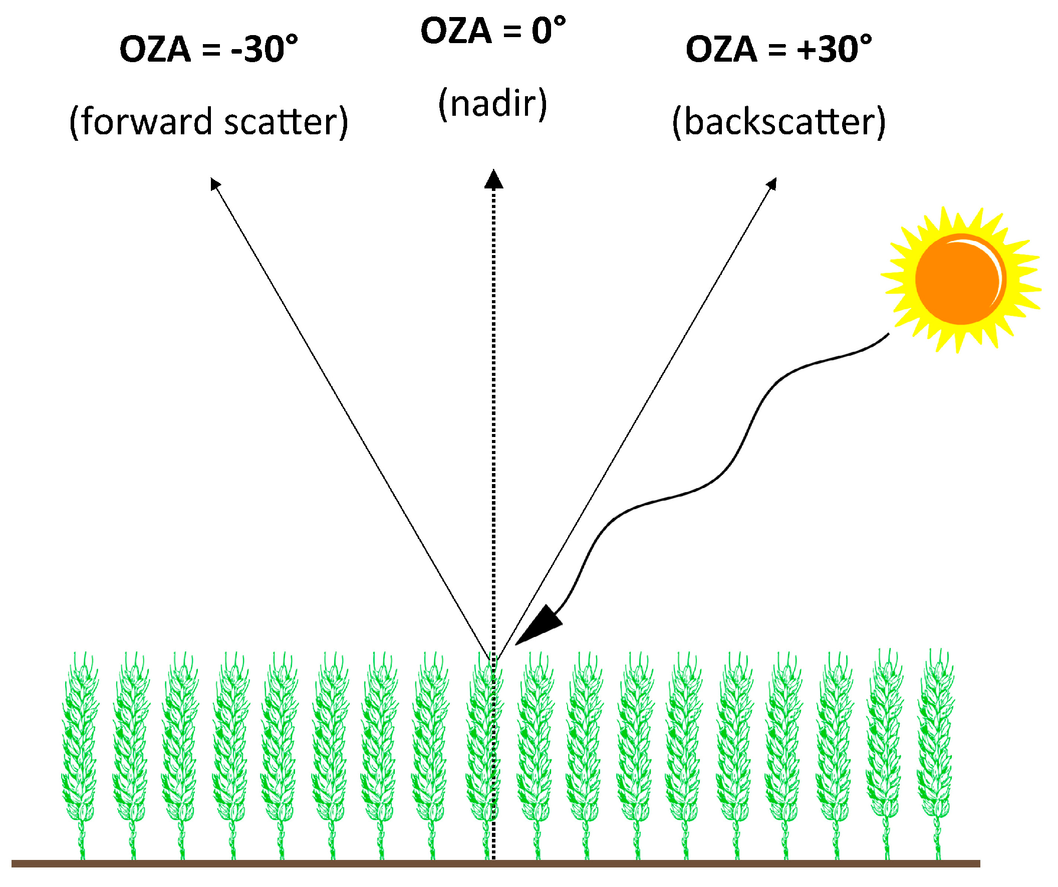
34]. Apart from nadir measurements, the canopy was also measured under observer zenith angles (OZA) of +30° and −30° regarding the solar plane: a sensor inclination towards the sun is defined as a positive OZA, whereas an inclination away from the sun is described as a negative OZA (
Figure 1). Due to the
backscatter effect, spectra with positive OZA are noticeably brighter than nadir views or negative zenith angles, as they draw nearer to the spot of increased backscatter, also known as the hot spot [
35]. The opposite direction shall accordingly be called cold spot or
forward scatter and usually leads to reduced reflectances and darker images. For the angular spectral measurements, a microphone stand was modified to hold the ASD glass fiber optic. The horizontal rod of the stand could be raised or lowered to adjust the viewing angle with help of an attached inclinometer. The observer azimuth angles (OAA) matched up with the row azimuth angle of the canopy stands (170° for field 517 and 150° for field 509). EnMAP will operate on a sun-synchronous orbit with 97.96° satellite inclination angle descending node [
36] which corresponds to an OAA of 187.96°. The angular effects measured in the presented campaign therefore are assumed to adequately represent the angular effects expected from future EnMAP data.
Spectral information from each of the 3 × 3 ESUs was compiled to pseudo-images with a ground sampling distance of 10 m. Furthermore, the processed signatures were converted into simulated EnMAP spectra via the EnMAP-end-to-end-Simulator (EeteS) [
37]. In this process, the sensor-specific radiometric and spectral properties were adapted. The spatial resolution in this case was retained at 10 m to preserve the data population.
The gap fraction is a measure for the probability of a ray of light to penetrate through the canopy undisturbedly [
38]. Accordingly, this parameter decreases with density and/or height of a canopy. Canopy height can also be seen as a path length on which energy can interact with plant traits. Assuming identical canopy height, the path length is shortest for nadir views and increases with OZA > 0°. For a 30° deflection from nadir, the travelled path is longer by factor cos (30°)
−1 which is 15.5%. This leads to a weaker influence of soil background and to an apparently higher portion of visible leaf surface.
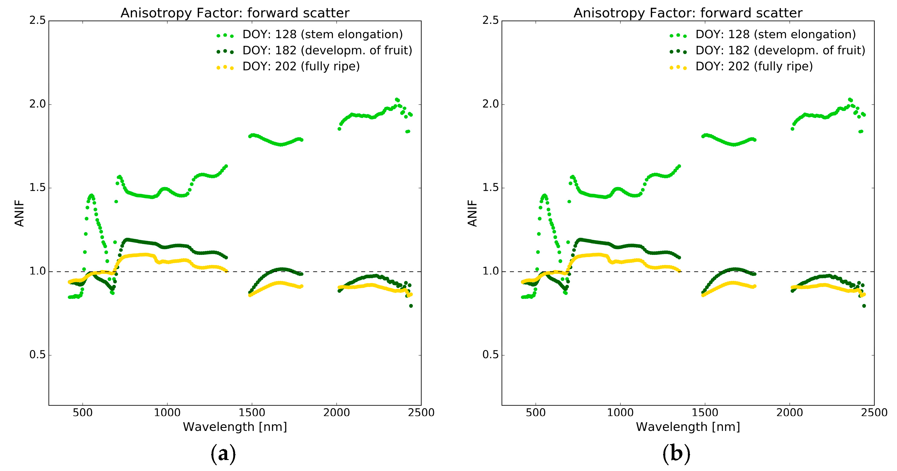
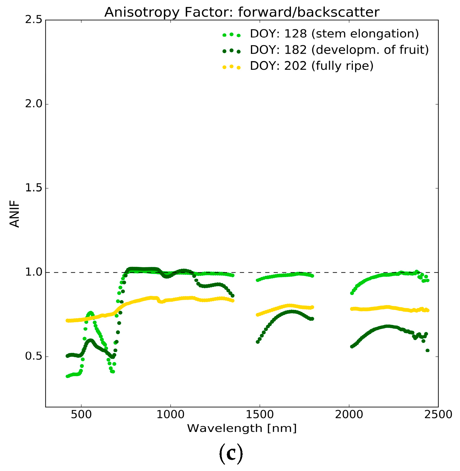
The anisotropy factor (ANIF) [
39] yields useful information about the sensitivity of different wavebands towards changes in illumination geometry. It is simply defined as Equation (1):
Since the experimental setup covers two different viewing directions, two ANIFs were obtained: one for forward scatter (ANIFfs) and one for backscatter (ANIFbs). Additionally, a third ANIFfs/bs was calculated as the ratio between reflectances per waveband in forward and backscatter direction.
If spectral information of the same target is available for multiple angles, it was found useful to combine them and thus raise predictability. This has been done with surface-near spectrometers that are handheld [
40], mounted on a tower [
41], on hemispherical devices [
42] or UAVs [
11]. A prominent example for multi-angular optical remote sensing from space is CHRIS/Proba which allows to record narrowband spectra in the VNIR-domain from five different viewing angles (e.g., [
43,
44]). EnMAP will be able to perform an across-track satellite tilt, but will keep up this slanting position for longer time than its view upon the target. If the same target shall be observed under different zenith angles, more than just one acquisition will have to be made with a time gap of at least several days or possibly several weeks or months. Canopy parameters that are strongly influencing the bidirectional reflectance distribution function (BRDF) change diurnally as well as during the seasonal growth cycle. For this reason, in this study we concentrated on single looks only, regardless of the possible improvement of results for a
combined multi-angular approach.
2.2.2. Biophysical Variables
Agricultural crop variables were measured at the exact same location where spectral signatures were recorded shortly before. The time offset between the variable sampling and the spectral sampling was 45 min on average and 60 min at maximum.
Average Leaf Inclination Angle (ALIA) was measured with a Suunto PM-5/360 inclinometer held along the leaf petiole to display its slope against the horizontal plane [
45]. The measurement was repeated at different positions of the leaf and for different leaves within the canopy. Additionally the Leaf Inclination Distribution Function (LIDF) was noted down for a more detailed description of the canopy architecture [
46]. Leaf chlorophyll content (LCC) was measured with a Konica-Minolta SPAD-502 handheld device at different heights with focus on the upper canopy layer. The chlorophyll meter had been individually calibrated in a preceding field campaign against destructive measurements of winter wheat leaf chlorophyll content from different senescence states. Coefficients of [
47] were used to derive LCC from the samples. Leaf senescence (C
br) was estimated as the fraction of brown leaf parts in the foliage. This variable varies between zero (no brown spots = 100% fresh vegetation) and one (no green spots = 100% senescent vegetation). For a proper estimation of C
br, the approach of [
48] was slightly adapted to incorporate the non-linearity of the vertical distribution of brown leaves. The dissociation factor between upper and lower layer thus created consistent results. This was achieved by applying a cosine function of the brownness in the upper layer to the power of two. C
br can be written as Equation (2):
with br
u as the fraction of brown leaf parts in the upper and br
l in the lower layer of the canopy. For LAI measurements, a LI-COR Biosciences LAI-2200 instrument was used that had been upgraded with the ClearSky Kit to obtain functionalities of the advanced LAI-2200C. Equipped with a GPS sensor and a white diffuser cap, the device allows for nondestructive measurements of leaf area index under sunlight conditions. To obtain green LAI, the measured LAI value was multiplied with the factor 1 − C
br to exclude the impact of non-photosynthetic vegetation on LAI measurements. Multiplication of leaf variables with the LAI value allows their interpretation on canopy level, e.g., canopy chlorophyll content (CCC).
2.3. Radiative Transfer Modelling
For this study, PRO4SAIL-5B (PROSPECT 5B + 4SAIL) was used which operates based on the input parameters listed in
Table 2 and described in
Section 2.2.2.
Following the suggestion of [
1], the Skyl-parameter was kept stable at 0.1. The soil brightness parameter scales the dominance of the bright and dark canopy background in the output signal. By default, standard literature soils are used for this. In this study they were replaced by the brightest and the darkest soil spectrum of the campaign, measured directly at the study fields for each date. The background signal gains more weight in the simulated reflectance for vegetation that is sparse in terms of green LAI. It is important to note that spectral signatures of senescent canopies differ from those of small plants that cover the soil only partially, although situations might result in the same low value for green LAI. For this reason, another background type is introduced that was calculated as the mean senescence signal for ripe wheat crops of both seasons. All other leaf and canopy parameters were randomly drawn from uniform distributions with min and max values adjusted according to
Table 2. Input parameters regulating the s–t–s-geometry uniformly covered all field scenarios. For example, the minimum SZA observed in the field was 29.14° and the maximum was 52.63°. As a result, SZAs of 30°, 35°, 40°, 45°, 50° and 55° were used for generating the LUT. Variations in the OZA of −30°, 0° and +30° took account of the three experiments of the simulated EnMAP platform tilt. For winter wheat crops it was suggested setting the leaf structure parameter N to a mean of 2.0 with a SD of 0.34 [
7]. Since our study data covered the complete vegetation cycle from seeding to harvest, these values were slightly adapted to a wider range of 1.0 to 2.5.
The size of each LUT (n
lut) can be understood as the number of variations of the parameters (n
para) multiplied by the number of variations of the s–t–s-geometry (n
angles). n
lut has a linear influence on the calculation time for the generation and the inversion of the LUT. On the other hand, larger LUT sizes yield more possible parameter constellations, which may improve the quality of the retrieval. Many authors suggest n
para = 100,000 as the best trade-off between calculation time and inversion accuracy (e.g., [
8,
12,
49]). In each of these studies, however, angles of sun and observer were fixed. As described in
Table 2, n
angles here needed to cover 252 different geometric constellations which would result in n
lut = 25,200,000 for each soil and senescence background. A LUT-size of 12,600,000 (n
para = 50,000) turned out to perform equally well (Δ
RMSE < 1%), while allowing a quicker inversion and thus the conduction of more experiments in the same period of time. Accounting for the different potential background signals (soil or senescent material respectively) the LUTs are duplicated and only varied by a different background signal. This method, therefore, shall be called duplex LUT.
Finally, artificial noise can be applied to make simulated spectra more realistic and to improve the inversion accuracy (overview given by [
6]). The best performing LUT settings have been varied in noise type (Gaussian additive/Gaussian inverse multiplicative) and noise level (0.0%, 0.1%, 1.0%, 2.0%, 5.0%, 10.0%) respectively.
2.4. Step-Wise Inversion of the LUT
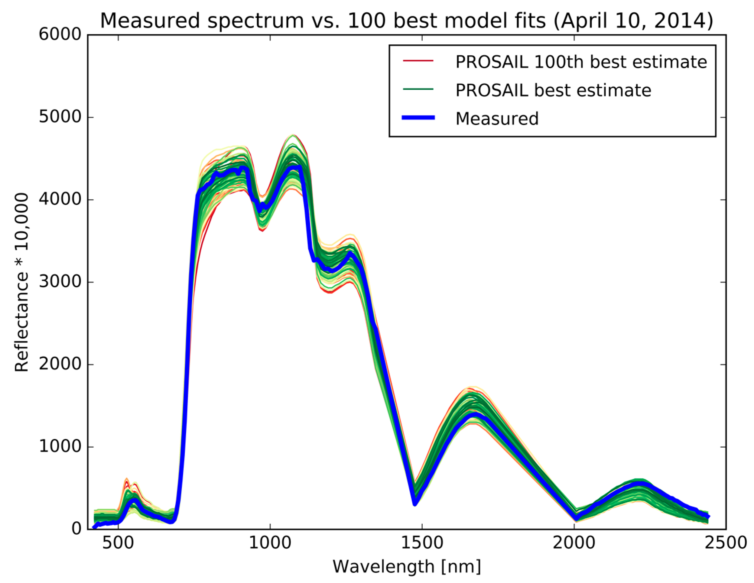
Inverting a LUT means comparing measured spectra with all PROSAIL model results and selecting the parameters that led to the best performing LUT members. Different cost functions can be used to quantify the agreement between measurement and model result. Most authors use the Root Mean Squared Error cost function type (RMSE
cft), defined as Equation (3):
By squaring the distances before extracting the root, larger deviations gain more influence in this term. Consequently, the RMSE
cft favors results for which both spectral signatures match rather closely for all wavelengths. An alternative cost function tested is the Nash-Sutcliffe-Efficiency (NSE
cft [
50]) as defined in Equation (4),
Weighing the squared sum of distances between measured and simulated reflectance against the squared sum of distances between measured reflectance and the average measured reflectance of the complete spectrum. The mathematically simplest approach is the mean absolute error (MAE) as defined in Equation (5):
In all three cases, Rmeasured(λi) is the measured and Rsimulated(λi) is the modelled reflectance at wavelength λ for the ith spectral sensor band, whereas n corresponds to the total number of bands used for the optimization.
For each sampling date, the s–t–s-geometry must be known. Prior to application of the cost function, the correct sub-LUT must be selected. At first, by analysis of the observed spectrum, the corresponding LUT is inquired, depending on the expected canopy background. Senescent vegetation does not only show distinct absorption features by leaf pigments, but also significant features in the SWIR domain. A new index that has been optimized for the EnMAP spectral configuration, the NPVI
EnMAP (Equation (6)) is introduced. NPVI
EnMAP is used to classify the background of a pixel as either soil (type A) or senescent vegetation (type B) based on a simple threshold.
If NPVIEnMAP < 1.4, the spectrum is classified as type B and classified as type A for all other cases. Based on the angular constellation for each pixel a decision is made, which of the remaining 252 sub-LUTs shall finally be used for the inversion.
The ill-posedness can be mitigated by narrowing the parameter constraints for the generation of the LUT. In this case, the user needs to have access to a priori information about the expected data range. These constraints make the approach more empirical and thus inconsistent with the proposed generic conviction of the study. For this reason, the ill-posed problem was dealt with by considering more than just the one best performing LUT member and its according parameter configuration [
3]. The final results vary with the number of considered best fits (n
bf). A tradeoff between singular (ill-posed) and multiple (over-balanced) solutions needed to be found for an optimal retrieval setup (n
bf ϵ {1, 20, 50, 100, 200, 500, 1000}). For n
bf > 1, the median is used to get the final parameter value.
Figure 2 illustrates the necessity to include an adequate amount of LUT-members for the variable retrieval. Parameter constraints for the creation of the LUT can be narrowed down to further increase inversion performance (e.g., [
42]). In doing so, the model is calibrated to site-specific characteristics and might not be able to help retrieve variables for other fields, crop types or phenological stages.
The step-wise hierarchical variable retrieval was achieved by several consecutive complete LUT-inversions. A motivation for this approach is the dominance of some parameters (e.g., LAI) that may suppress the signal of others (e.g., LCC) affecting similar spectral domains. For the first inversion run, all available spectral bands were included except for those influenced by the atmospheric water vapor absorptions (1359 nm–1465 nm and 1731 nm–1998 nm) and the VNIR-bands in the detector overlap of the EnMAP-HSI (911 nm–985 nm). Although all variables were obtained in this first step, LAI was the only one of interest at that time. The average inclination of leaves is an important regulation parameter that describes the visibility of photosynthetically active parts of the vegetation for the sensor. Erectophile canopies reveal larger parts of the underlying soil, especially for low SZAs. Planophile and plagiophile canopies on the other hand cover more of the background and lead to stronger signals just like an increased LAI would. ALIA and LAI therefore counterbalance each other. In an attempt to separate their influences on the measured spectra, another pre-selection is investigated for the first inversion run, selecting only those LUT members with an ALIA close to the one estimated in the field.
For the second inversion run, the LAI values resulting from the first run were fixed. A pre-analysis selected only those LUT members containing the retrieved LAI ± an absolute tolerance of 0.01 (m² m−2). If this pre-selection left fewer members than two times the size of nbf, the valid tolerance was expanded by increments of 0.01 until the minimum condition was met. Only then the second run was started during which LCC was retrieved by separately applying the cost function to the variable-specific sensitive wavelengths (LCC @ 423–705 nm).
According to the authors of [
51] the performance of an inversion setting shall ideally be assessed by multiple statistical quality criterions when comparing retrieved model parameters to in situ measured values. Most importantly, the relative Root Mean Squared Error (rRMSE) and the slope of the regression line (m) were considered in this study. The coefficient of determination (R²) played a minor role, since it measures the strength of the correlation according to the linear regression rather than the 1:1 relationship between model parameter and in situ variable. A regression model was calculated nonetheless and its slope served as an indicator of the inversion accuracy. A slope of 1.0 suggests a perfectly outbalanced relationship. Slopes > 1.0 reveal an underestimation for low and overestimation for high values. The reverse relationship applies for slopes <1.0. For all following analyses, model runs with a slope <0.7 or >1.3 were not considered in the final results.
4. Discussion
For the interpretation of directional angular effects on spectral reflectance, the anisotropy factor (ANIF) can be consulted: due to self-shading effects, forward scatter images appear darker than nadir or backscatter images. In the latter case, a greater fraction of incident sunlight is reflected back to the direction of its origin and is consequently missing on the opposite viewing direction. This so-called hot spot effect leads to a spectral saturation and superimposes parts of the signal of leaf constituents. Moreover, ANIF is highly correlated with the magnitude of reflectance itself. If the canopy reflectance is higher, discrepancies increase between nadir and forward scatter but decrease between nadir and backscatter. On the other hand, if more radiation is absorbed or transmitted by the canopy, anisotropy decreases for forward scatter and increases for backscatter. Spectrally, high anisotropy occurs for blue and red portions of the solar spectrum from which leaf chlorophyll mainly absorbs radiation to photosynthesize. This was also found by [
52] for both directions, but in our study this could only be confirmed for backscatter mechanisms. This phenomenon may be the reason why it was more difficult for the PROSAIL model to reproduce the measured spectra from this direction, leading to a weaker estimation of LCC from backscatter in comparison to forward scatter spectra.
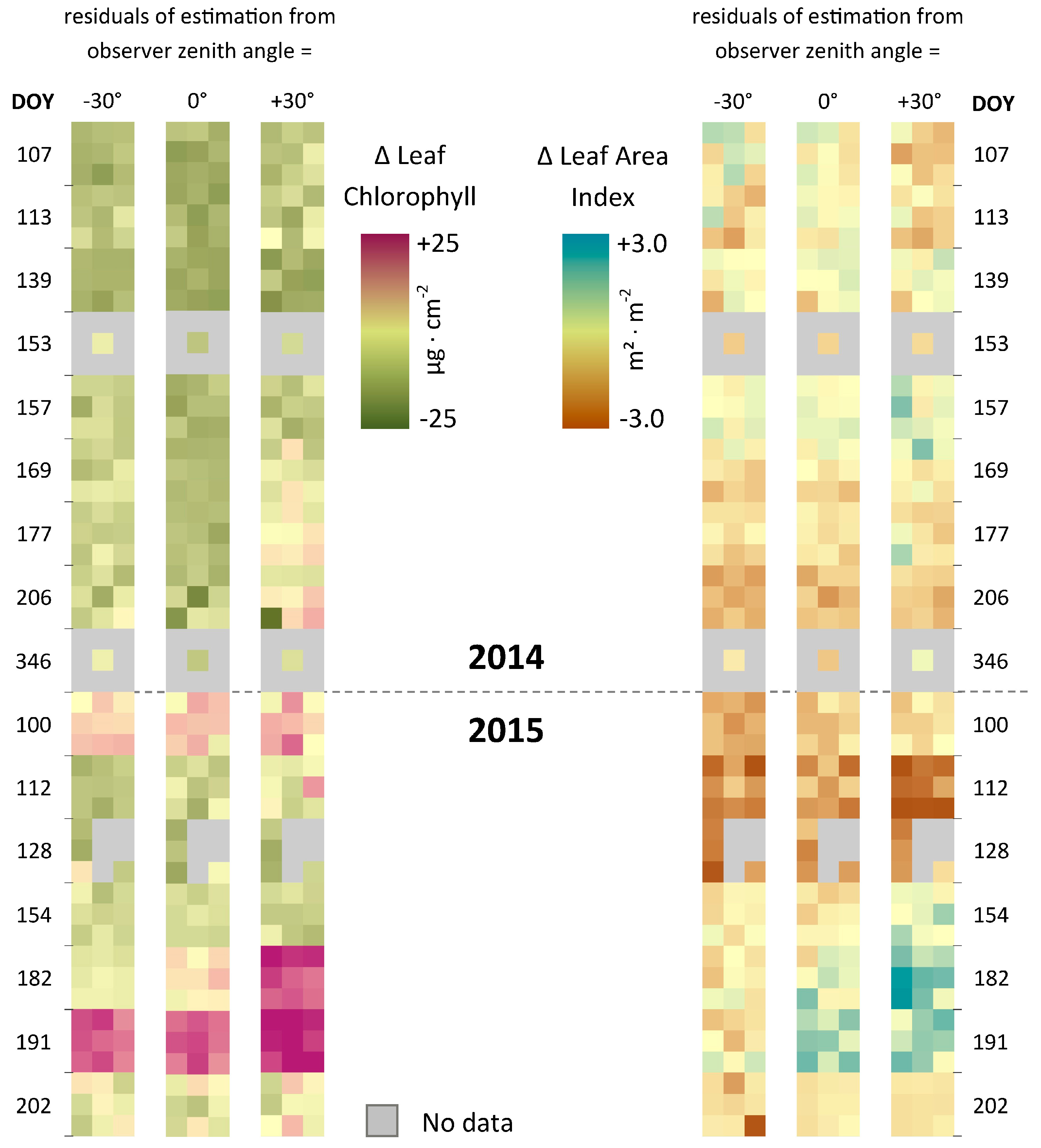
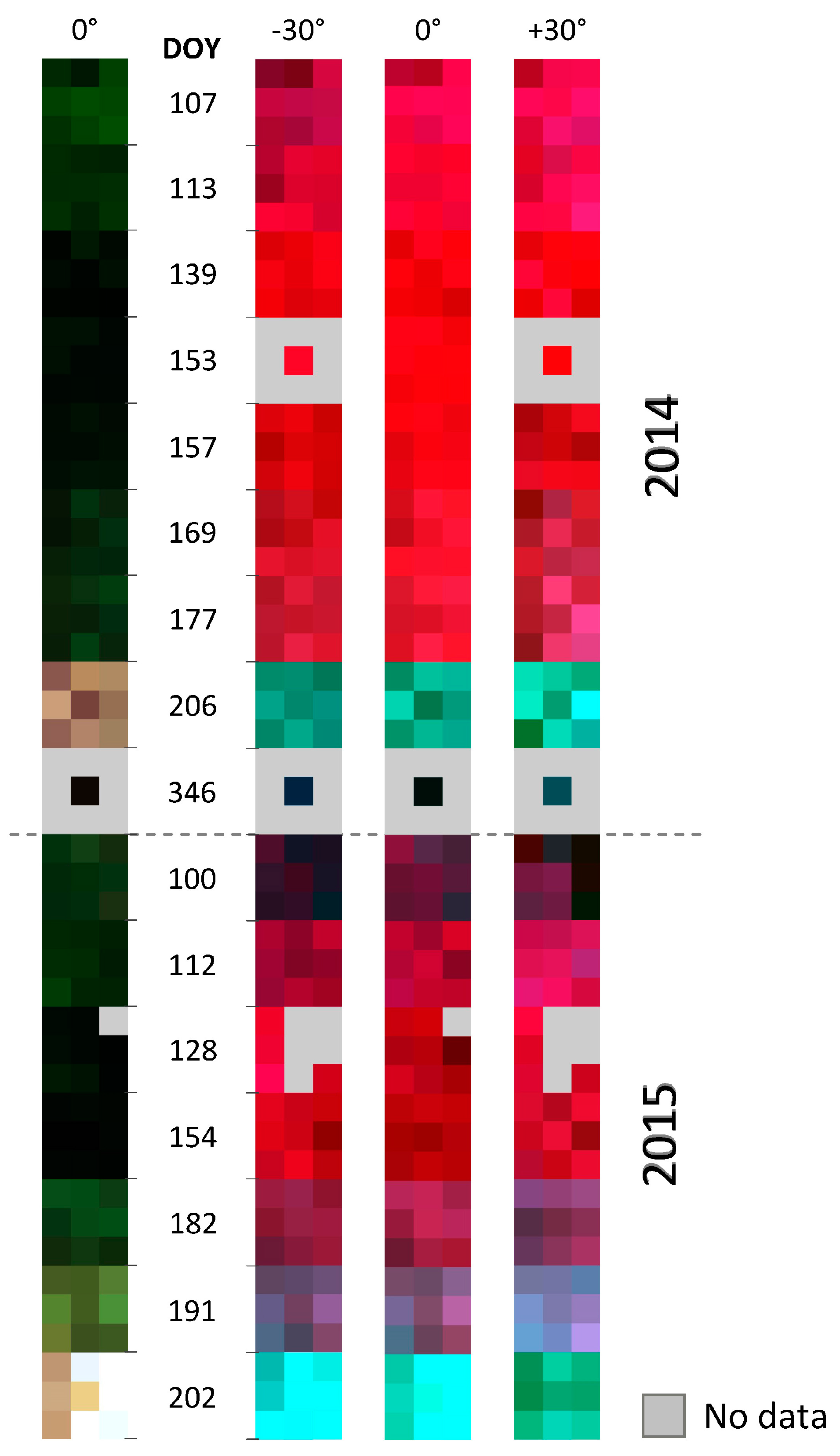
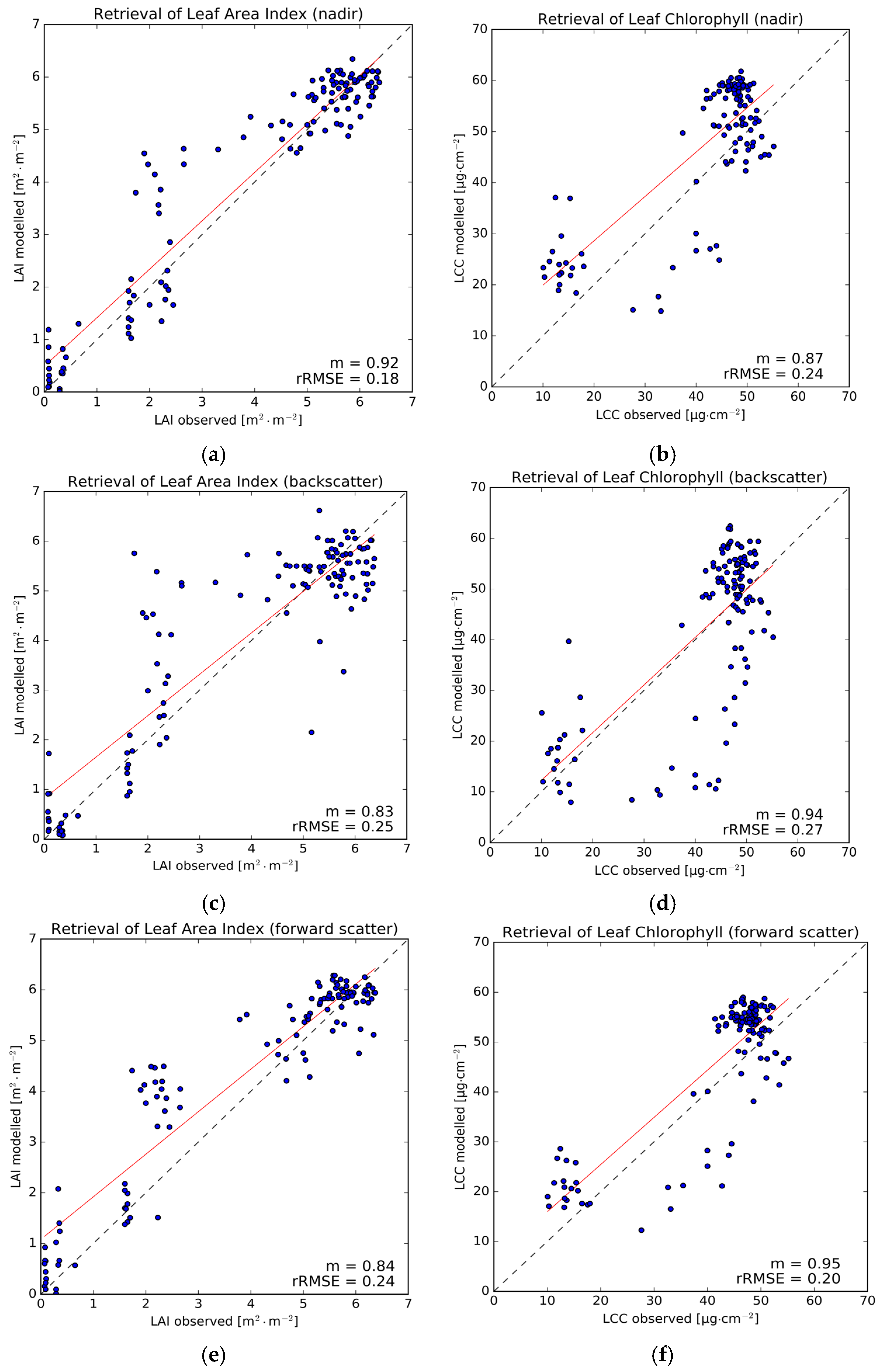
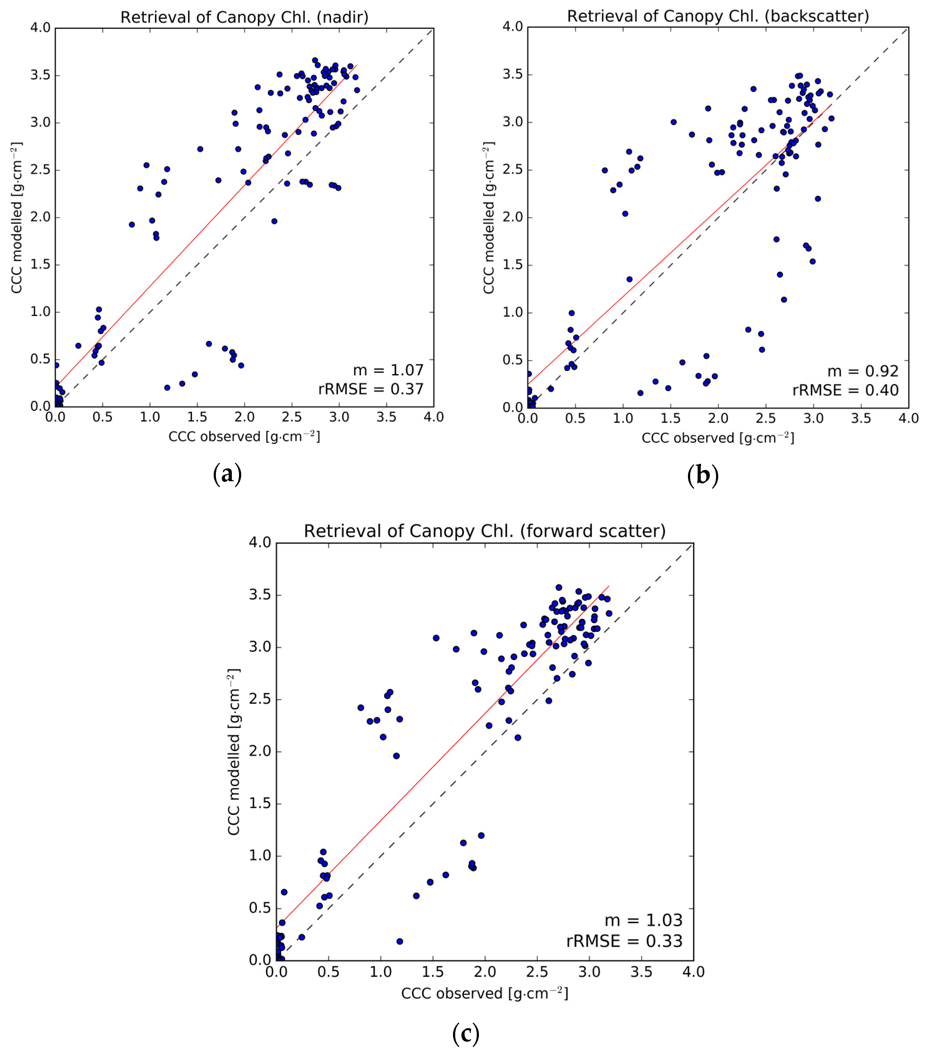
Our main study objective was to assess the effect of off-nadir observations on the prediction accuracy for leaf and canopy variables, namely LAI and leaf chlorophyll content, as it will have major implications for the user community of future EnMAP data. Generally, for both off-nadir observations, accuracy decreased when estimating LAI: rRMSE = 18% at nadir vs. rRMSE = 25% (backscatter) and rRMSE = 24% (forward scatter). For LCC and CCC, the off-nadir mode with forward scatter yielded highest accuracies with rRMSE = 20% and rRMSE = 33% respectively. Once again, the complex structure of the canopy plays an important role for the output of PROSAIL. Turbid medium assumptions are best met for homogeneous crops with least possible complexity in plant structural traits. Winter wheat is thought to be particularly well suited for a representation through RTMs [
19]. Nevertheless, the leaf surface of wheat exhibits anisotropic reflectance that is mathematically described by the BRDF [
40]. Backscattering leads to glare effects and thus complicates the retrieval of LAI. In the opposite direction, i.e., forward scatter OZAs, the canopy appears darker which seems slightly better suited for the retrieval of LAI. If EnMAP data is only available for backscatter observations, an inversion will still be successful, but the user will encounter larger uncertainties.
Leaf glint generally leads to a reduced accuracy for the inversion of LCC. Senescent plant material absorbs less of the incident radiation and is more subjected to hot spot effects [
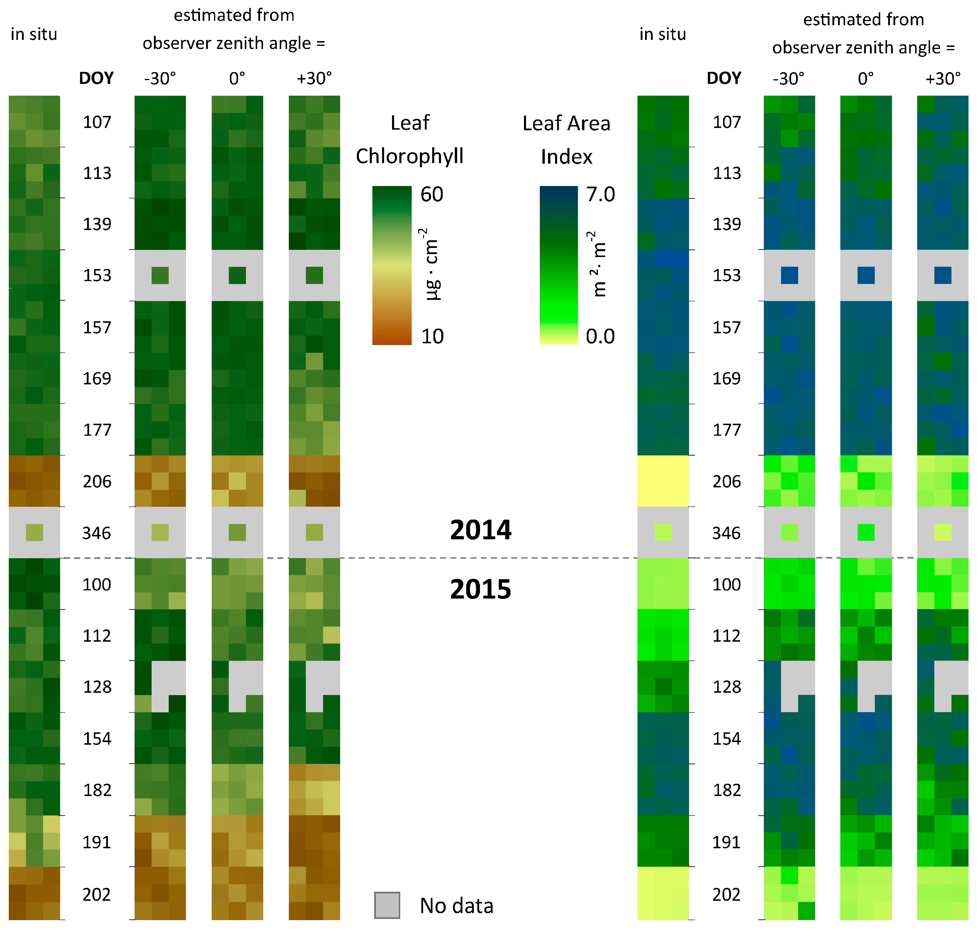
53]. This could be confirmed (see
Figure 5), as LCC > 40 μg cm
−2 was poorly estimated from backscatter spectral images, but well inverted from forward scatter observations. The findings suggest that LCC is best retrieved, the greater the difference of the zenith angle between sun and observer becomes. CCC acts like a linear combination of LAI and LCC in any statistical analysis. The rRMSE for nadir appears to be comparatively high and the intercept of the linear model is t = 0.20 which is 10.6% of the data average. This constant overestimation is caused by the before mentioned overestimation of LAI and LCC from nadir spectra reducing the models accuracy. An improvement of the retrieval of these two parameters also yields an improvement for CCC, as can be seen for results from the forward scatter observations.
Another focus of this work was to test different LUT-based strategies, while keeping a special focus on the zenithal-angular effects for spectral observations from the future EnMAP sensor. Most commonly, the RMSE
cft is used as a merit function to find the best matching LUT members. In fact, there is only a 3.0% mean difference between RMSE
cft and MAE in the resulting parameter estimation. The n
bf to incorporate in the parameter retrieval has a much stronger impact on the success of the inversion. If we assess only the rRMSE as a statistical measure for the inversion performance, it could be concluded that for LCC there is a steady improvement in predictability for larger n
bf. It should be noted, however, that the slope responds conversely, decreasing for larger n
bf and moving away from the optimal value of 1.0. Lower regression slopes indicate that the range of predicted variables becomes more level, cutting off lowest and highest inversion results. Sehgal et al. [
54] found an optimal inversion routine with n
bf = 10% of the LUT-size which, in their case, was 5400 members. For larger n
bf the inversion approaches the expected value of the variable as specified before the creation of the LUT, so RMSE is bound to decrease if field observations served as a reference for the original parameter distribution. For all angular settings, statistics deteriorated for n
bf > 100 or 0.2% of the compared LUT-members. This suggests that the LUT composition was optimally set. Accordingly, n
bf = 100 is considered as the optimal setting in the case of this study.
A comparison of the performance with other studies is generally difficult, due to the exploration of different sensor data, LUT-compositions, inversion techniques, crop types and measurement ranges. However, as example, Atzberger et al. [
7] retrieved LAI with an RMSE of 0.83 (m² m
−2) and CCC with RMSE 0.66 (g m
−2) from winter wheat spectra by training artificial neural networks on PROSAIL which is roughly in the same accuracy range as our findings for nadir observations.
Different sources of errors and uncertainties in the whole inversion process must be considered as limitations to this study: in situ measurements of biophysical variables, spectral measurements, simulation of EnMAP data, model representation and the inversion scheme. For most variables, in situ errors can be reduced by choosing an adequate sampling scheme with multiple repetitions. The median standard deviation for LAI measurements of two seasons was 0.22 (m² m
−2) and 3.16 (μg cm
−2) for LCC. Repetitions of the ALIA estimation in the field revealed a mean error of ±7°. Senescent canopies yielded higher uncertainties for the measurement of most variables. Standard deviation of all EnMAP-end-to-end simulations was σ = 0.013 (Refl.) at the NIR-plateau which is 0.28% of the mean reflectance at this wavelength. In comparison to other error sources, this uncertainty played only a minor role. LAI acts as a scaling factor for the leaf constituents. The reflectance signal is ambiguous for substances of lower concentrations within a dense canopy or substances of higher concentrations in a sparse canopy respectively. The hierarchical approach estimates LAI first, fixates it and then finds the other parameters in consecutive inversion steps. This proved to work well for LCC, but not yet for other parameters. For instance, ALIA could not be estimated despite its high sensitivity throughout the covered spectral range [
55]. Early in the development of PROSAIL it was stated that ALIA and LAI are highly correlated and therefore can hardly be separated in the inversion [
56]. In fact, if LAI is inverted with an accuracy of 20%, there is no autocorrelation (R² < 0.01) of the ALIA residuals, although the parameter itself could not be retrieved in any acceptable way. For an improvement of leaf pigment estimations, the new version of PROSPECT (Prospect-D [
57]) is eagerly awaited for a more detailed representation of the leaf-biochemistry, namely the consideration of anthocyanins.


