1. Introduction
Remote sensing images obtained by remote sensing imaging systems, are widely used in understanding and management in landscape ecology, natural resource planning, and environmental systems. Super-resolution remote sensing can be considered as an inverse problem that reconstructs a high-resolution (or fine-resolution) image from a set of coarse-resolution class fractions [
1,
2]. However, due to the physical limitation of relevant imaging devices in remote sensing, scaling up ground and remotely sensed data to the desired spatial resolutions, is unavoidable [
3]. For super-resolution reconstruction of continua in remotely sensed images, Atkinson et al. [
4] studied the downscaling cokriging, which provides an incremental development for the use of cokriging for image fusion described in Ref. [
5]. Boucher and Kyriakidis [
1] proved that many approaches for remote sensing using super-resolution adopted prior models of spatial structure, either implicitly or explicitly (see for example Ref. [
6]). Boucher et al. [
2] also proposed a geostatistical solution for super-resolution of remote sensing images using sequential indicator simulation to obtain multiple possible stochastic results. Pan et al. [
7] proposed a super-resolution reconstruction method of remote sensing images based on compressive sensing, structural self-similarity, and dictionary learning. Generally speaking, super-resolution reconstruction is a process of combining one or multiple low-resolution spatial images to produce a high-resolution image, and is a powerful tool to acquire the desired spatial resolution in remote sensing.
Various super-resolution methods have been proposed, which can be categorized into three classes [
8,
9,
10]: interpolation-based methods [
11,
12,
13], multi-image-based methods [
14,
15,
16], and example learning-based methods [
17,
18,
19,
20]. The interpolation-based methods apply a base function or an interpolation kernel to predict the pixels in high-resolution grids. However, they only perform well in smooth (low-frequency) areas, but poorly in edge (high-frequency) areas. The multi-image-based methods recover a high-resolution image by fusing a set of low-resolution images of the same scene, but they are restricted by the difficulties of acquiring enough low-resolution images.
The last category of super-resolution methods is based on example learning, assuming that the lost information in a low-resolution image can be learned from a set of training images [
21]. Training images are numerical prior models containing the structures and relationships existing in realistic models. The example learning-based methods acquire a high-resolution image by inferring the mapping relationship between the high-resolution and low-resolution image pairs, so a set of high-resolution training examples should be prepared in advance for learning. Obviously, this kind of method heavily relies on the quality of the training image sets.
To address the super-resolution issue based on example learning for remote sensing, one can use a prior model to limit the under-determination caused by missing or incomplete spatial information. Once the prior model of spatial structures has been determined, it provides a probability distribution of corresponding variables studied in above super-resolution issue. Actually, the probability distribution hidden in the prior model contains the uncertainty about the unknown attribute values to be reconstructed given the current available conditional information. Also, the uncertainty in probability distribution may lead to multiple results providing an assessment of uncertainty regarding remote sensing images, instead of generating only one single image from the conditional data [
1,
2].
As one of the main branches of stochastic simulation, and introduced by the seminal work of Guardiano and Srivastava [
22], multiple-point statistics (MPS) is a relatively broad concept, allowing capture of intrinsic structures from a prior model existing in a training image, and then copying them to the simulated region by reproducing high-order statistics conditioned to some conditional spatial data. Hence, MPS can fully use the given prior information and conditional data simultaneously [
23,
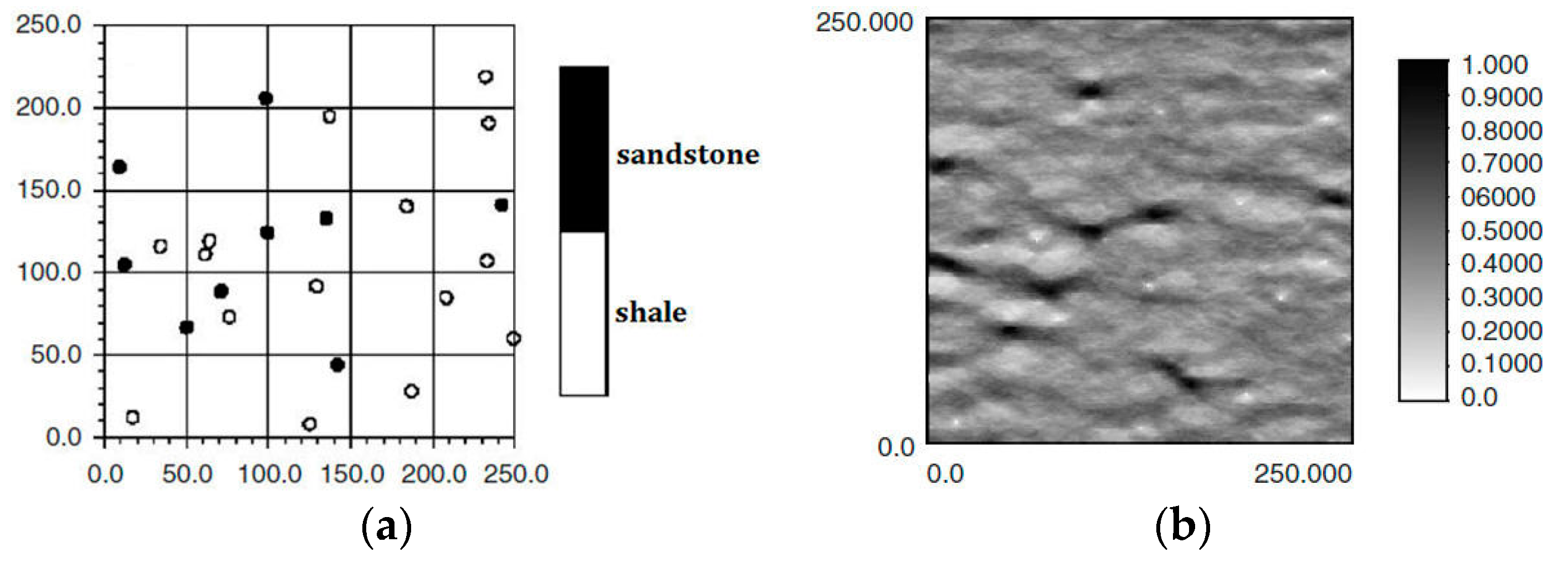
24]. In MPS, there are two types of conditional data to limit the simulated results: hard data, and soft data. For example, in the characterization of oil wells,
Figure 1a,b is, respectively, hard data and soft data in the same region (250 × 250 units). The white and black points in
Figure 1a are shale wells, and sandstone wells, respectively, with
Figure 1b describing the probability of sandstone hidden in the whole region. Soft data are usually abundant and much easier to be achieved than hard data, so they especially should be used for reconstructing the unknown models for better precision.
In addition to conditional data, another issue challenging MPS is that it is normally quite CPU-intensive, due to its large computational burden. Hence, some classical MPS methods, like filter-based simulation (FILTERSIM) [
23], and distance-based pattern simulation (DISPAT) [
24], use dimensionality reduction to decrease the redundancy existing in high-dimensional data extracted from training images, hopefully reducing the burdens of computation. In FILTERSIM, the patterns in training images are characterized by some filters to acquire the filter-based score space. DISPAT introduces multi-dimensional scaling (MDS) for dimensionality reduction of training images. Although MDS in DISPAT and filters used in FILTERSIM can reduce the dimensionality and help to discover the linear structures of training images existing in high-dimensional space, they fail to reconstruct nonlinear structures, because they essentially are linear dimensionality reduction methods.
Normally, those structures with strong correlations in high-dimensional space can generate some results that lie on or close to a smooth low-dimensional manifold that is widely studied in differential geometry, as well as machine learning, known as “manifold learning” [
25,
26,
27,
28]. As a classical method in manifold learning for nonlinear dimensionality reduction, isometric mapping (ISOMAP) preserving geometry at all scales replaces Euclidean distances by geodesic distances, mapping nearby points on the manifold to nearby points and faraway points to faraway points in low-dimensional space [
28].
The aim of this paper is to present an example learning-based method using MPS and ISOMAP for super-resolution of remote sensing images. Because of the capability brought by ISOMAP in nonlinear dimensionality reduction, ISOMAP is combined with MPS to be qualified for the functions as MDS in DISPAT, or filters in FILTERSIM. Besides, soft data are quite useful for improving reconstruction quality, so coarse fraction data from low-resolution images are used as soft data for reconstruction in our method. The remainder of this paper is organized as follows.
Section 2 details the explanations for each step of the proposed method.
Section 3 summarizes the main procedure of the method.
Section 4 provides comparative experimental results, and
Section 5 concludes this paper.
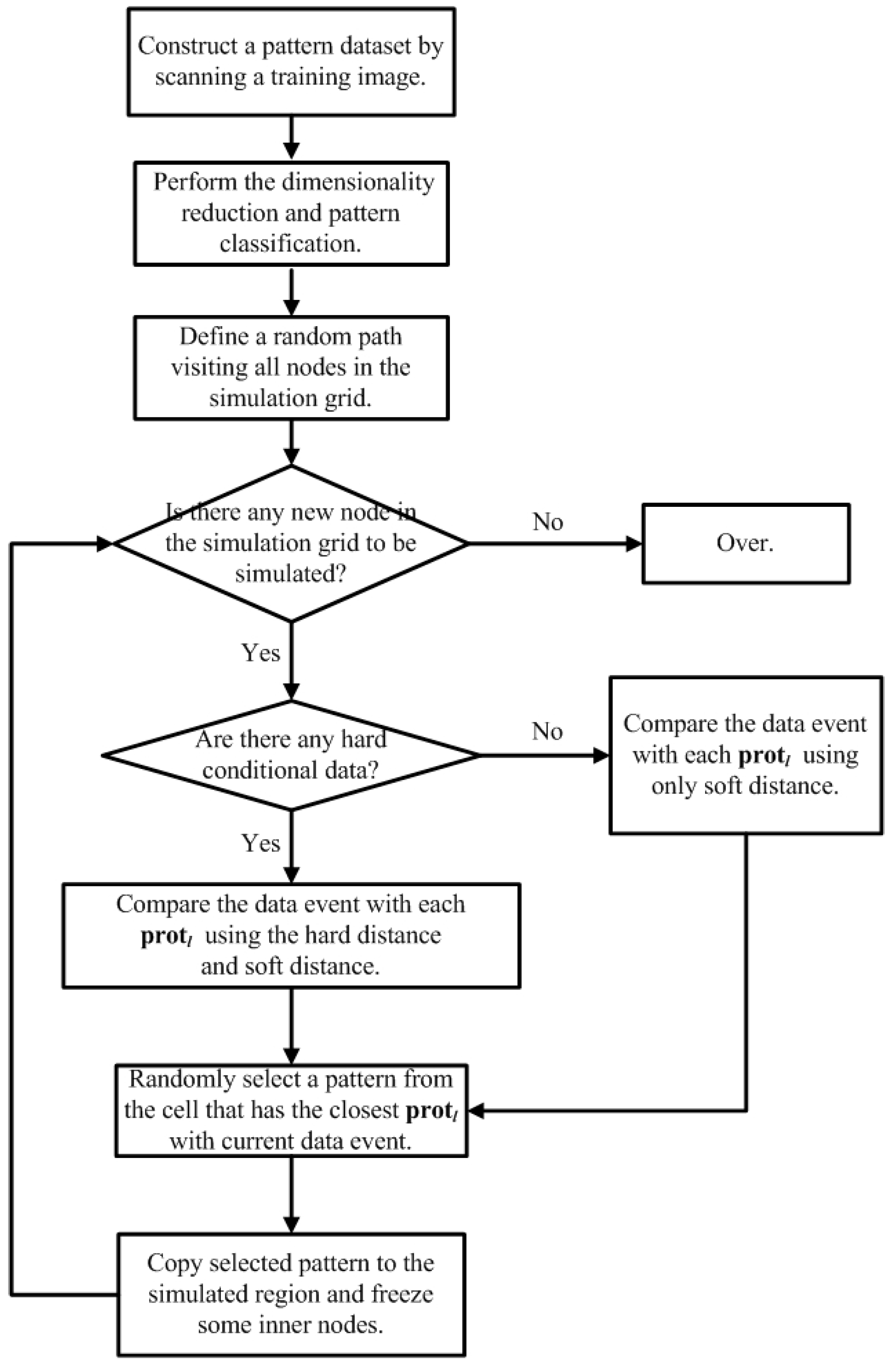
2. Detailed Explanations for Each Step of the Proposed Method
There are in total, 4 steps in the proposed method, which will be described in the following sections.
2.1. Step 1: Building a Pattern Dataset from Training Images
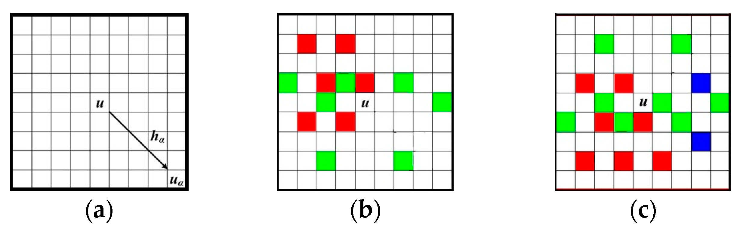
2.1.1. Data Templates, Data Events and Patterns
A training image is scanned with a data template τ
D that comprises a central location
u, and its
D neighboring locations
uα(α = 1, 2, …,
D).
uα is defined as
uα =
u +
hα, where
hα is the vector describing the data template. Considering that an attribute
S has
J possible states {
sk;
k = 1, 2, …,
J}, the data event
d(
uα) with the central location
u is defined as [
29]
where
S(
uα) is the state at the location
uα within τ
D, and
means one of the states of
sk.
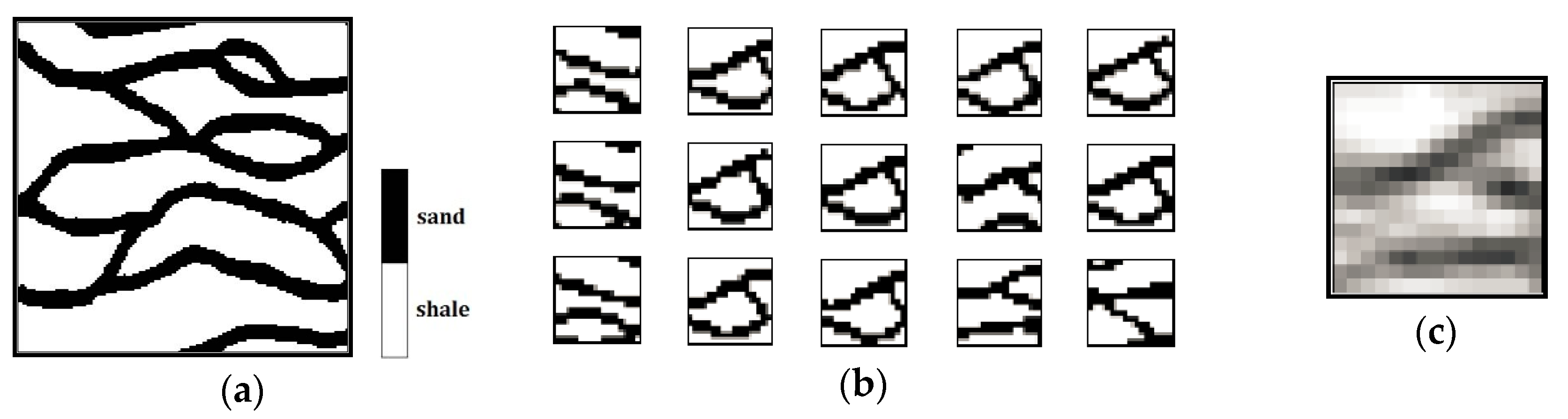
Figure 2a illustrates a data template with 9 × 9 nodes, in which the central node
u is to be simulated.
Figure 2b,c are two data events captured by τ
D. The different nodal colors in
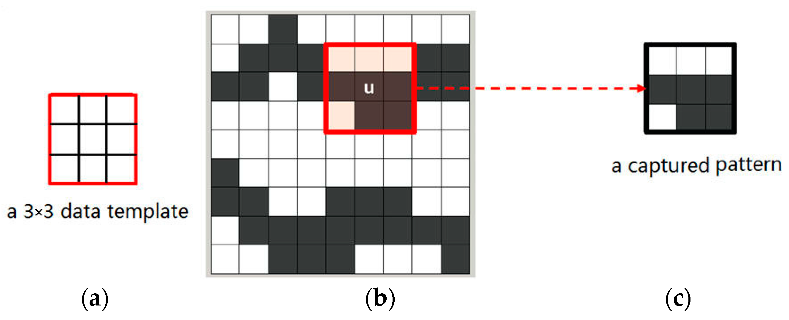
Figure 2b,c mean different states of an attribute. Non-color square means the state of current node is unknown. Note that the term “node” here means a pixel in a 2D image. The data events extracted from training images are also called “patterns” representing the essential features of training images. For example,
Figure 3 illustrates a pattern of a training image captured by a 3 × 3 data template. Only two states, the white node and the gray one, exist in the training image of
Figure 3b.
2.1.2. Building a Pattern Dataset
Normally a pattern dataset should be constructed before dimensionality reduction. For MPS simulation, all patterns should first be properly extracted from a training image. Each pattern means a point in high-dimensional space. A training image is scanned with τ
D, and
ti(
u) is defined as a pattern centered at
u, and captured by τ
D in a training image. Let
ti(
u +
hα) be the state at
u +
hα, so
ti(
u) can be defined as follows:
Extract all patterns from a training image and let them be location-independent, so that one can get the
k-th pattern:
where
Npat is the total number of captured patterns, and each
patk(
hα) corresponds to
ti(
u + hα) (α = 1, 2, …,
D). Therefore, the pattern dataset
patDb can be described:
where each
patk (
k = 1, 2, …,
Npat) means a point in high-dimensional space.
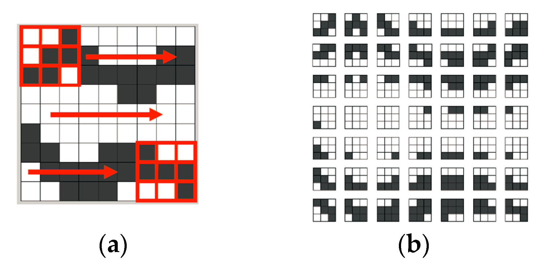
Figure 4a shows the process of τ
D (displayed with a 3 × 3 pixel grid) scanning over a gray-and-white training image. τ
D moves only one-pixel (or one-node) distance for each capture, from left to right in each row.
Figure 4b is the captured pattern dataset [
24].
2.2. Step 2: Dimensionality Reduction of Patterns by ISOMAP
Each patk has D elements, so it can be considered as a point in a D-dimensional space. Our plan of dimensionality reduction is to map each patk to a d-dimensional space (d << D), while the intrinsic relations and characteristics in patk will be well maintained. Therefore, the whole process of dimensionality reduction can be depicted as follows: the pattern dataset patDb that includes Npat patterns patk (k = 1, 2, …, Npat, patkD) will be mapped using ISOMAP from a D-dimensional space to a d-dimensional one, and then a new dataset Y(=(y1, y2, …, ), ykd), is acquired. Each yk has a much lower dimensionality, but the number of patterns remains unchanged after dimensionality reduction. The process of dimensionality reduction using ISOMAP is:
2.2.1. Step 2.1. Construct Neighborhood Graph G of Patterns
Compute all the Euclidean distances between all pairs of data points to be used as an approximation to geodesic distances. Define the Euclidean distance between
pati and
patj as
dE(
pati,
patj):
If patj is one of the k nearest neighboring patterns of pati, draw a line between patj and pati in G. By repeating this step, one can get the neighborhood graph of pati by drawing lines between the remaining k − 1 nearest neighboring patterns, and pati. For each pati(i = 1, 2, …, Npat), one can finally acquire the neighborhood graph G.
2.2.2. Step 2.2. Find Out the Shortest Path dM(pati, patj) between Two Patterns
If
pati and
patj are directly linked by only one line within a neighborhood, initialize
dM(
pati,
patj) =
dE(
pati,
patj); otherwise
dM(
pati,
patj) =
. Note that above
dM(
pati,
patj) is only an initialization of distance, and may be replaced by a smaller value in the subsequent computation using the following Equation (6). For each
p = 1, 2, …,
Npat, define the shortest path as
The matrix of shortest path distances can be defined as
DM = (
dM(
pati,
patj))
2,
i,
j = 1, 2, …,
Npat. The whole procedure of computing the shortest path by Equation (6) can be considered as the well-known Floyd’s algorithm that can acquire the shortest path in a weighted graph [
30]. Because Equation (6) is a recursive procedure, “
dM(
pati,
patp) +
dM(
patp,
patj)” in Equation (6) can lead to
dM(
pati,
patp) finding the shortest path between
pati and
patp, and similarly,
dM(
patp,
patj) finding the shortest path between
patp and
patj, respectively. Such recursive procedure continues, and finally the shortest path
dM(
pati,
patj), can be obtained. Even if initially
dM(
pati,
patp) =
, or
dM(
patp,
patj) =
, after limited times of recursive procedures,
dM(
pati,
patp) and
dM(
patp,
patj) can be obtained by Equation (6).
2.2.3. Step 2.3. Compute the d-Dimensional Mapping
Compute the following symmetrical matrix
where
I is an
Npat-dimensional identity matrix, and
l is an all-one
Npat-dimensional column vector. Compute
B’s largest
d eigenvalues λ
1 ≥ λ
2 ≥…≥ λ
d, whose corresponding eigenvectors are
α1,
α2, …,
αd. Define
(
m = 1, 2, …,
Npat;
p = 1, 2, …,
d) as the
m-th component of
αp. Then, the target
d-dimensional matrix is
where
ym is the vector of the
m-th component of each
, i.e.,
ym = (
,). After mapping from
patDb = {
patk} (
patkD,
k = 1, 2, …,
Npat) to
Y = {
yk} (
ykd,
k = 1, 2, …,
Npat), the dimensionality of patterns has been reduced from
D to
d.
The dimension of the low-dimensional space, i.e.,
d, is a key parameter for ISOMAP: if the dimension is too small, important data features are overlapped onto the same dimension; if the dimension is too large, the projections become unstable.
d is derived by the maximum likelihood method in this paper (for more details, see Ref. [
31]).
2.3. Step 3: Classification of Patterns
After the dimensionality reduction is finished, the mapping of patterns in low-dimensional space
d should be classified. Any clustering method can be applied to the classification of patterns, such as partitioning methods, hierarchical methods, and density-based methods. The notion of a cluster, as found by different algorithms, varies significantly in its properties. There is no objectively “correct” clustering algorithm, but each one has its own application fields. The most appropriate clustering algorithm for a particular problem often needs to be chosen experimentally, unless there is a mathematical reason to prefer one cluster model over another [
32]. The classical k-means is chosen as the clustering method in this paper. Given an input number of clusters, the k-means algorithm finds the optimal centroid of each cluster, then assigns each pattern to a specific cluster according to an input distance [
33].
After being clustered by k-means, the whole
d-dimensional space is divided into some small cells. Suppose
L and
l are, respectively, the total number and sequence number of non-empty cells. For each cell, a prototype
prot(l)(
hα) that has the same size with the data template is defined as the average of the pattern located at
hα in the
l-th cell:
where
cl is the number of patterns in the
l-th cell;
(
i = 1, …,
cl) is the center of a data template in the
l-th cell;
T means a training image, and
T(
+
hα) is the state of a training image at
+
hα. The average vector of the
l-th cell’s prototype is
which is considered as a representative for all patterns in the
l-th cell.
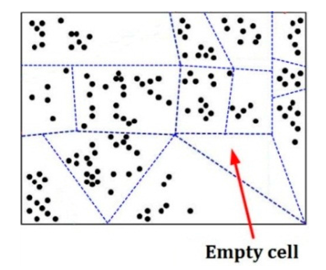
For example,
Figure 5 is an example of separating a
d-dimensional pattern space into some cells represented by some dotted-line surrounded regions, in which there is an empty cell, and each black point means a pattern in this space.
Figure 6a shows a training image containing sand channels in a shale background;
Figure 6b shows 15 patterns belonging to one cell;
Figure 6c is the average of all these 15 patterns, namely the prototype of this cell.
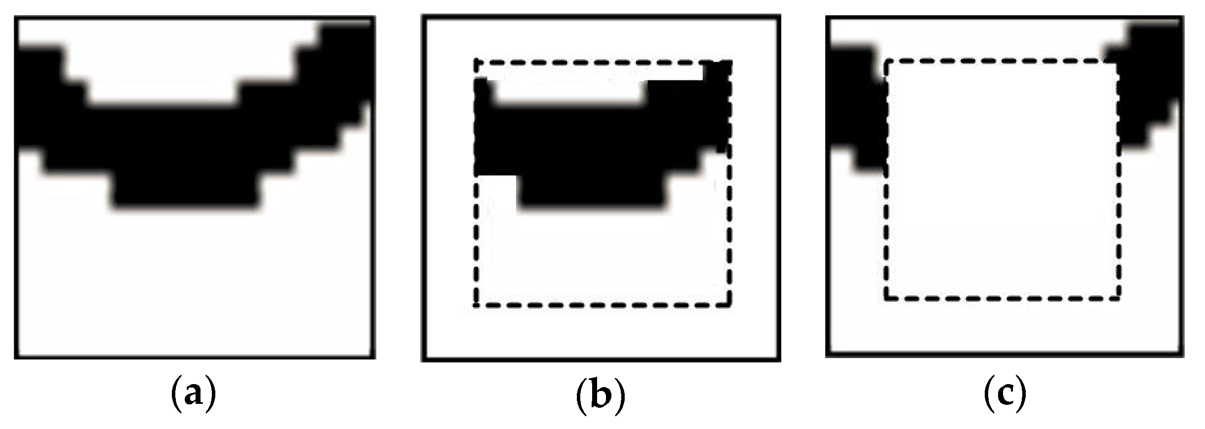
2.4. Step 4: Extraction of Patterns
When extracting a pattern, this pattern is divided into the inner (frozen) part, and the outer part. Both parts are viewed as hard conditional data for the simulation of next node along the simulation path, but the difference is that only the nodes in the outer part will be resimulated. Normally the inner part is set to a square in the pattern; the remaining part contains the outer nodes.
Figure 7 shows the two parts of a simulated pattern.
Considering
t as the data type, all nodes are divided into three categories: original known conditional data (
t = 1), frozen data used as conditional data that will not be resimulated (
t = 2), and simulated data that will be resimulated (
t = 3). Each node is assigned with a different weight,
, to measure its importance for computing distances according to its data type. At each node along the visiting path, the distance function
dis(
d(
uα),
protl) representing distances between data event
d(
uα) (i.e.,
d(
u +
hα)), and
protl, is calculated by comparing each known nodal value in the data event with each prototype
prot(l)(
hα):
where
is the weight of nodes with
. Clearly the original known conditional data have the highest weight. Note that the dimensionality reduction in
Section 2.2 is only used for the classification of patterns in
Section 2.3, and when extracting patterns, the distance in Equation (11) is calculated in the original space, but not the dimensionally reduced space.
In the super-resolution reconstruction of remote sensing images, coarse fraction information existing in low-resolution images is considered as soft data to constrain the reconstructions; hence the soft data always exist in the simulation procedure from the beginning to the end. The simulated nodes in the reconstructed region are both the results of super-resolution reconstruction, and the hard data for the unknown nodes in the subsequent simulation. It is seen that at the very beginning, since there are no any hard data in the region to be reconstructed, the reconstruction only depends on the coarse fraction information used as soft data. However, when the soft data and hard data are both available, consider the hard data event centered at
u as
hd(
uα), and its “hard distance” with each
protl is
where
is the
l-th hard distance, and
dis(·) means the distance calculation using Equation (11). Then the hard distance vector between
hd(
uα) and each
protl is
As for soft data, similarly define the “soft distance” between the soft data event
sd(
uα) and each
protl as:
where
is the
l-th soft distance. Then the soft distance vector between
sd(
uα) and each
protl is
According to Equations (13) and (15), the integration distance
Distotal of soft distance and hard distance is
where the distance vectors of
Dishd and
Dissd should be normalized into [0, 1] beforehand,
perhd is the percentage of known nodes in the current data event, μ (0 ≤ μ ≤ 1) is related to the ratio of the area already reconstructed (called
Arear) to the total reconstruction area (called
AreaT) and is defined as
Consider that
then
Distotal also is defined as
One can achieve the minimum among , , …, . Let R be the sequence number of this minimum. A patch patsel randomly chosen from the R-th cell corresponding to protR will be pasted to the region to be simulated, except the frozen locations, and locations corresponding to original known hard data. Then, freeze some inner nodes that will not be resimulated, and move to the next node in the simulation path, until all the nodes are simulated.
Note that coarse fraction information from low-resolution images is used as soft data, and this situation exists in the whole reconstruction, but hard data are not always existent. First, the super-resolution reconstruction proceeds with only soft data but hard data are not existent, so the distance computation in Equation (16) is only the calculation conditioned to the coarse fraction information to obtain Dissd. When the reconstruction continues, more simulated nodes (pixels) are available to be hard data. Then Equation (16) becomes a real combination of calculating Dishd and Dissd, meaning using soft data and hard data simultaneously.
4. Experimental Results and Analyses
4.1. Evaluation Method of Reconstruction Quality
MPS reconstruction is quite different from the non-stochastic reconstruction methods when evaluating reconstruction quality. When reconstructing the high-resolution remote sensing images from low-resolution images, MPS generates multiple stochastic results that provide an assessment of uncertainty regarding the true remote sensing images, as opposed to the single image solution frequently adopted in practice. Hence, it is impossible to achieve exactly the same simulated results with the training image when using MPS. MPS captures the features of a training image by copying its statistically intrinsic structures. It does not require the stochastic simulated results to be completely identical with the training image.
A variogram can be used to measure the similarity between simulated results and the training image, which is also the correlation between any two points in space when their separation increases, so it is used for evaluating the super-resolution reconstruction of remote sensing images. A variogram relates a variable at an unsampled location from its near locations, which is
where
Z(
u) and
Z(
u +
h), respectively, denote the estimators of the variable
Z at locations
u and
u +
h;
h is the lag distance;
E means mathematical expectation [
34].
4.2. Case Study
The experiments were run on a computer with an Intel core i3-4160T (a 3.1 GHz CPU) and 4 GB memory. The programming software was Matlab 2010. For parameters in Equation (11), = 0.5, = 0.3, and = 0.2. The template size is 17 × 17 pixels, and its inner part is 9 × 9 pixels. The capability of the proposed method to reproduce the super-resolution information of remote sensing images is demonstrated, hereafter, via a few categorical and continuous reconstructions of synthetic and real cases. The main objective is to illustrate that the prior structural features existing in the training images can be successfully generated in the super-resolution remote sensing images by our method. Note that these case studies are not to make the most locally accurate super-resolution remote sensing images for the particular region, but to generate multiple super-resolution reconstructions of remote sensing images from the available coarse resolution information, which can be used for some uncertainty assessment of risk evaluation, or decision making, that will not be discussed in this paper.
4.2.1. 2D Categorical Simulation
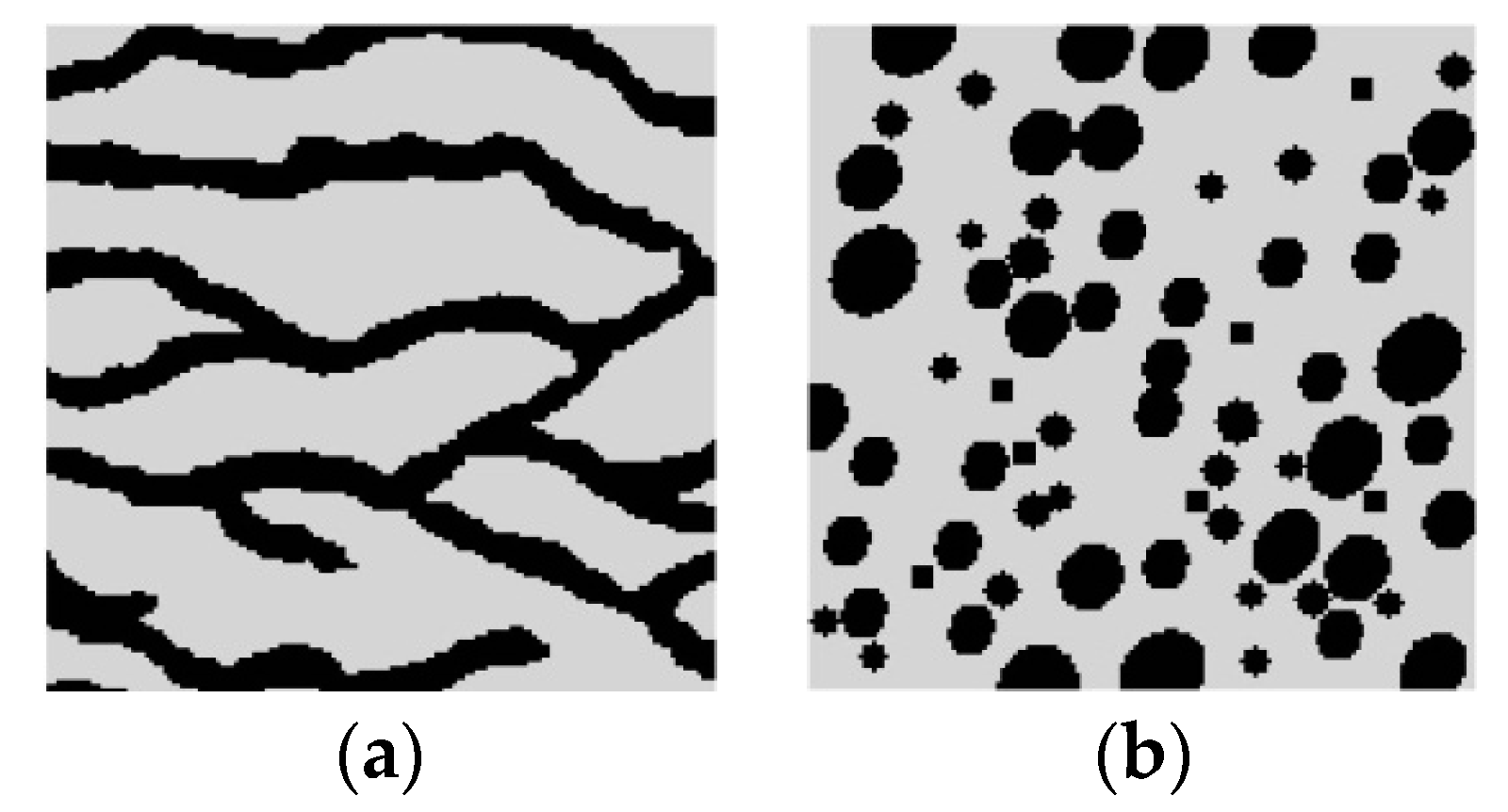
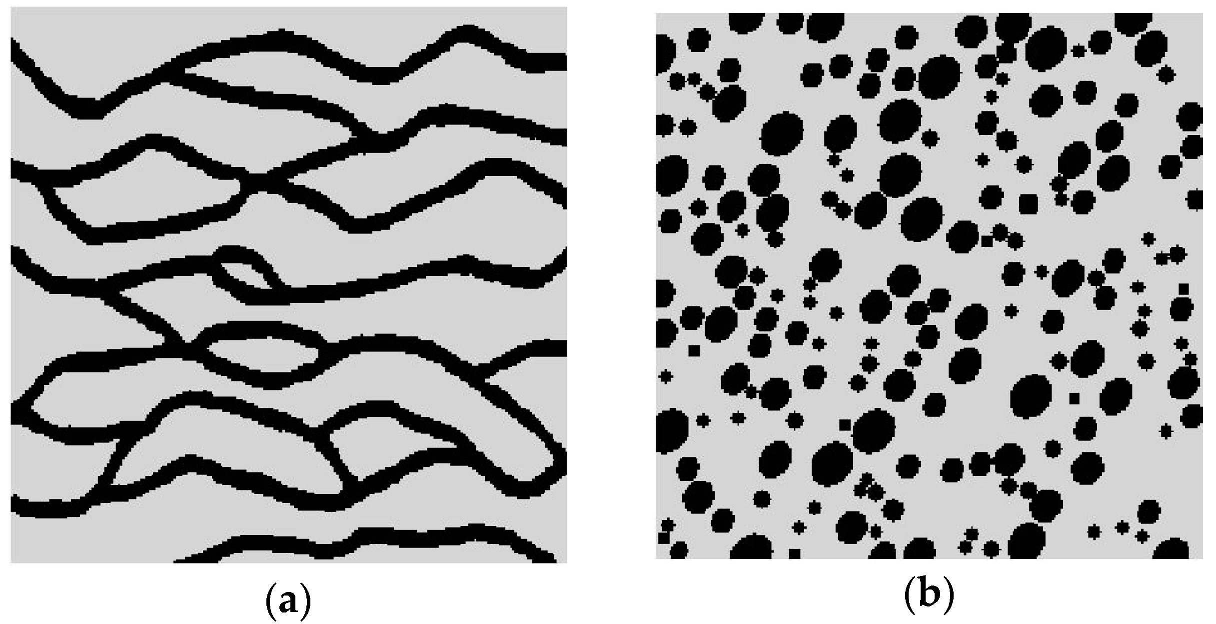
Super-resolution reconstructions for categorical variables are tested in this section. It should be noted that the training images and reference images considered in this categorical case are simply chosen for illustrative purposes. In the real-world applications, the true remote sensing images may be more complex, and contain more kinds of variables or classes. Consider two synthetic binary reference images, shown in
Figure 9a,b, each of size 150 × 150 pixels. These images are hereafter called Cases #1, and #2, respectively. Case #1 shows typical curvilinear shapes in a fluvial region. Case #2 shows a region filled with round shapes (including bigger ellipses and smaller circles), and few speckles. Set the black pixels (i.e., pixels representing the curvilinear shapes in Case #1, and round shapes and speckles in Case #2) to attribute value 1, and the gray pixels (representing the background in above two cases) to attribute value 0. The average of
Figure 9a,b are 0.27 and 0.30, respectively. The lower dimension
d, is set to 3 for both Case #1 and Case #2, derived by the maximum likelihood method.
The reference images of
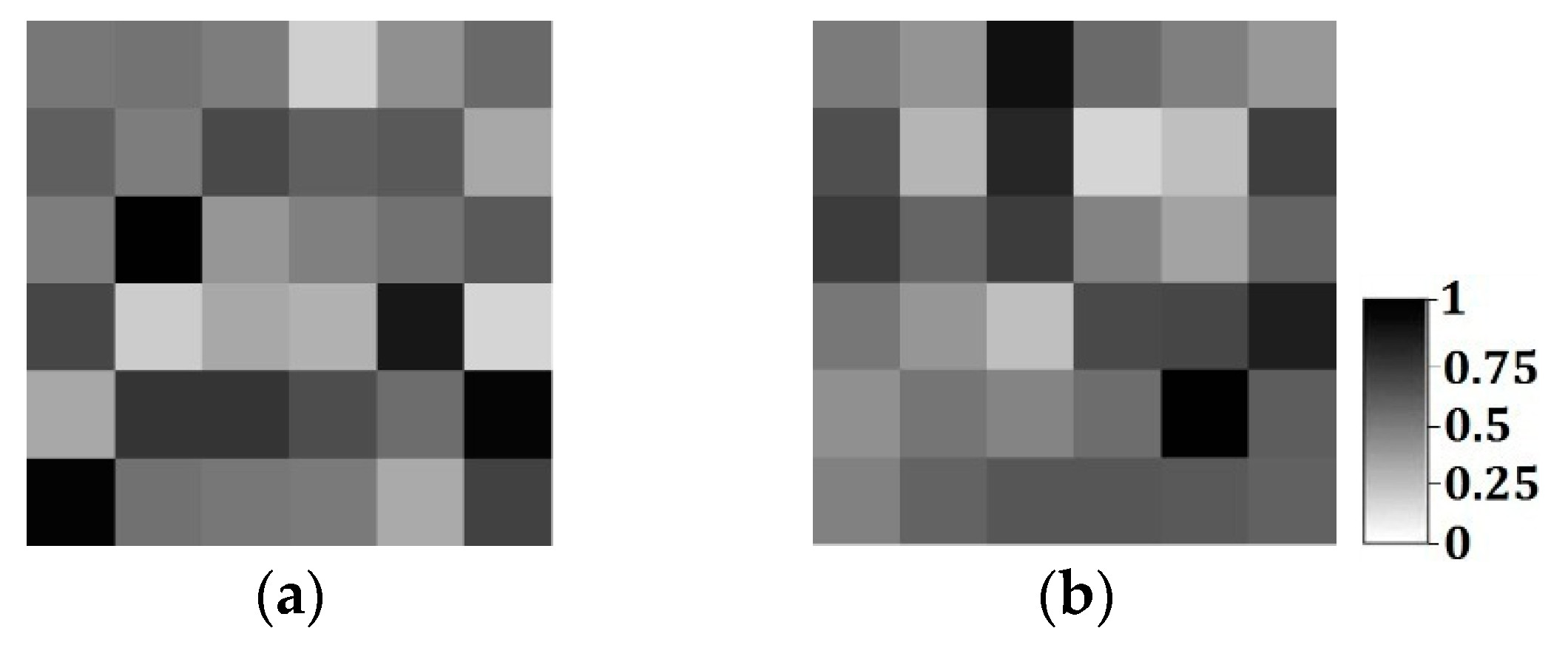
Figure 9 were then upscaled into two coarse fraction images using two different coarse resolution ratios. For each coarse pixel, the corresponding fractions were computed as the linear average of the fine pixel values within that coarse pixel. The coarse fraction images for Cases #1 and #2, with different resolutions computed from each reference image, are shown in
Figure 10 and
Figure 11, respectively. These coarse fraction images in
Figure 10 were computed by linearly averaging the reference images in
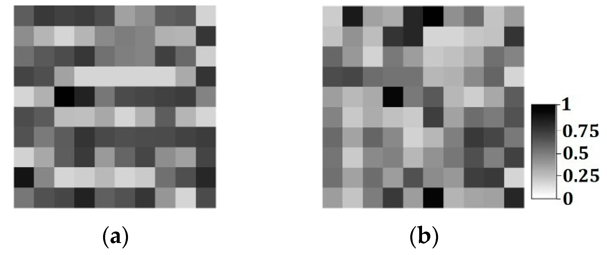
Figure 9 into blocks of 25 × 25 fine pixels each, creating images of 6 × 6 coarse pixels. Similarly,
Figure 11a,b were linear averages of the reference images in
Figure 9, with blocks of 15 × 15 fine pixels each, creating images of 10 × 10 coarse pixels. For
Figure 10 and
Figure 11, each coarse pixel is retrogressively comprised of 25 × 25 = 625, and 15 × 15 = 225 fine pixels, and the whole image is progressively comprised of 6 × 6 = 36, and 10 × 10 = 100 coarse pixels. Obviously
Figure 11 has higher resolution than
Figure 10.
Two training images for Cases #1 and #2 with 250 × 250 pixels are shown in
Figure 12. The prior structural models contained in the training images can constrain the reconstruction. Note that the training images and reference images have different sizes and are not identical, but they share similar patterns. In the following super-resolution reconstruction, our method was tested with the aid of coarse fraction information, meaning
Figure 10a and
Figure 11a were used as soft data, respectively, for Case #1 to reproduce the super-resolution reconstructed images with coarse fractions of two different resolutions (6 × 6 and 10 × 10 coarse pixels), and the prior structural features were extracted from
Figure 12a, that was used as the training image; also
Figure 10b and
Figure 11b were used for the super-resolution reconstruction of Case #2, with two coarse resolutions (6 × 6 and 10 × 10 coarse pixels) respectively, and accordingly
Figure 12b was the training image.
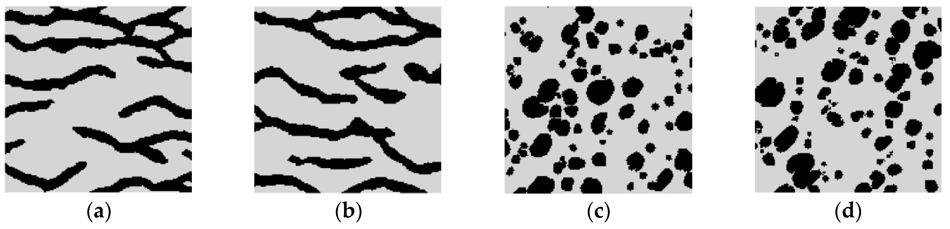
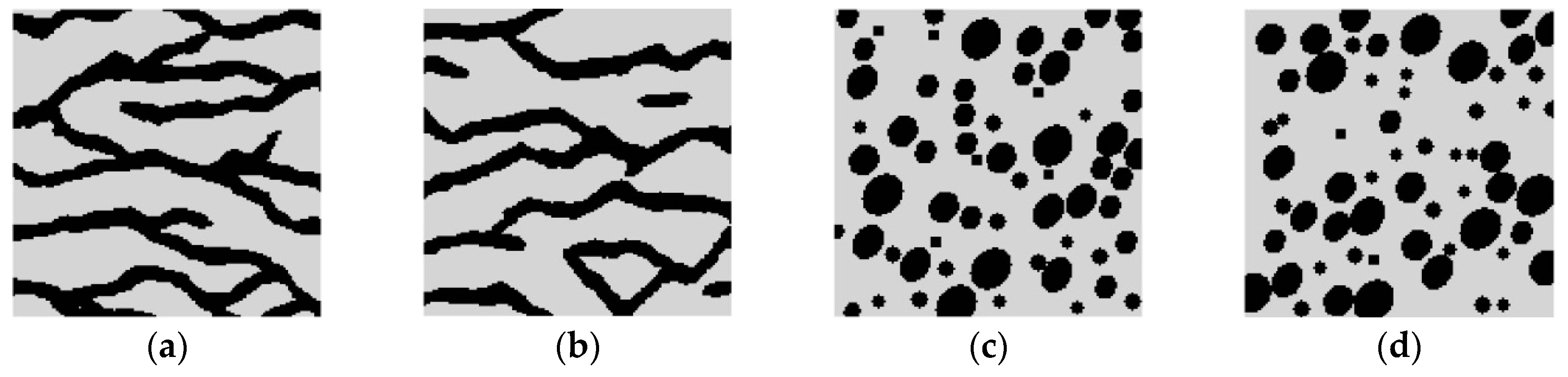
One hundred super-resolution realizations for Cases #1 and #2 were respectively generated, with different coarse fraction data, and some of them are shown in
Figure 13a–d and
Figure 14a–d. It is seen that each reconstruction reproduces the structural features in
Figure 9. However, the images generated with higher-resolution coarse fraction images (i.e.,
Figure 11a,b) clearly have better reconstruction quality. For example, in
Figure 14a,b, the curvilinear shapes have fewer intervals, but in
Figure 13a,b, the shapes are more disconnected. It also can be observed that in
Figure 14c,d, each ellipsis and circle are more complete and isolated, but many ellipses and circles are overlapped and irregular in
Figure 13c,d.
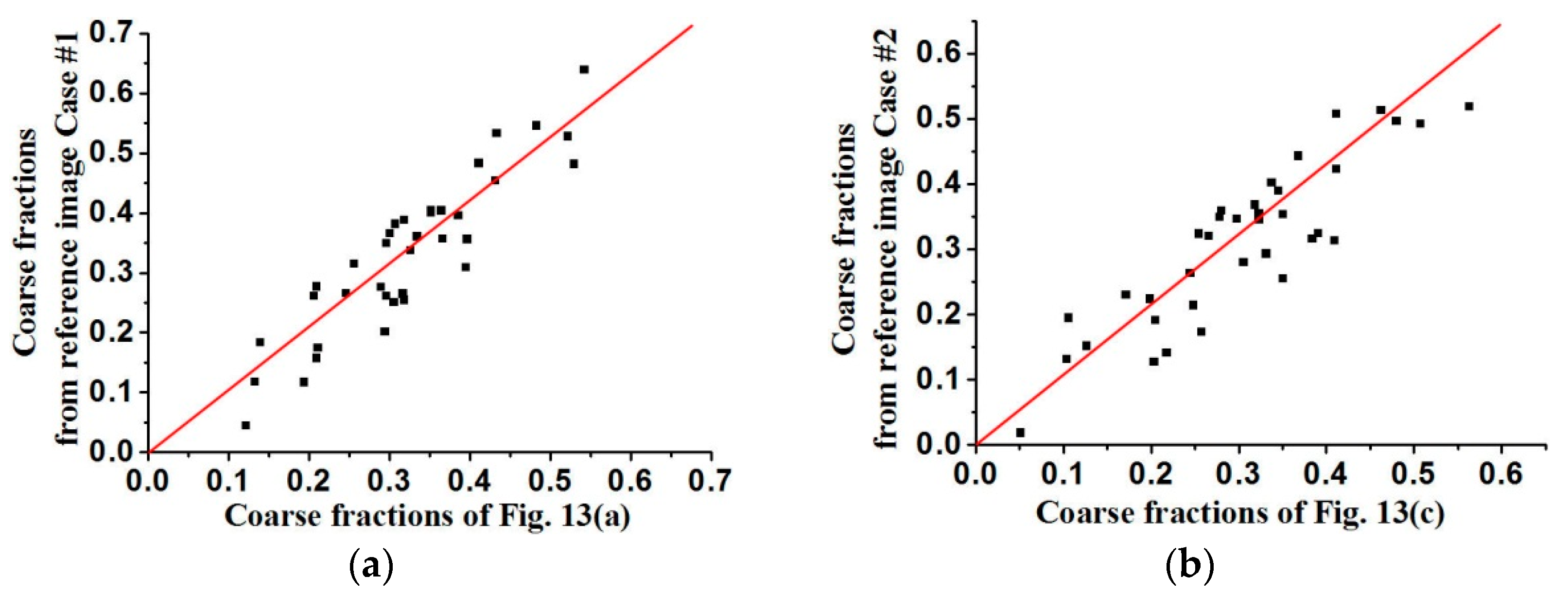
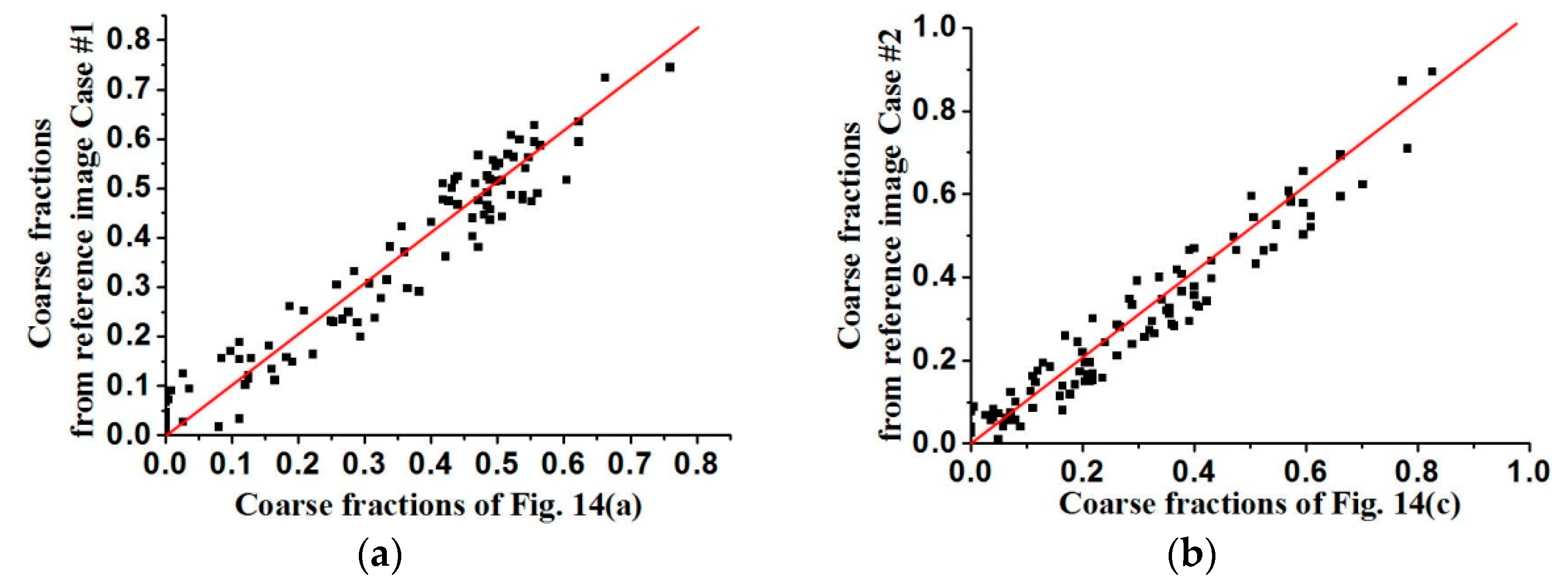
The coarse fraction reproduction is corroborated in
Figure 15 and
Figure 16, respectively, where the averages of coarse fraction images computed from the super-resolution reconstructed images are plotted against the coarse fraction data of reference images (a 45° line indicates good reproduction). The fluctuation of all the points near the 45° line indicates the good reproduction of coarse fractions in reconstructed images, but currently it is hard to find out which situation, meaning use of
Figure 13 and
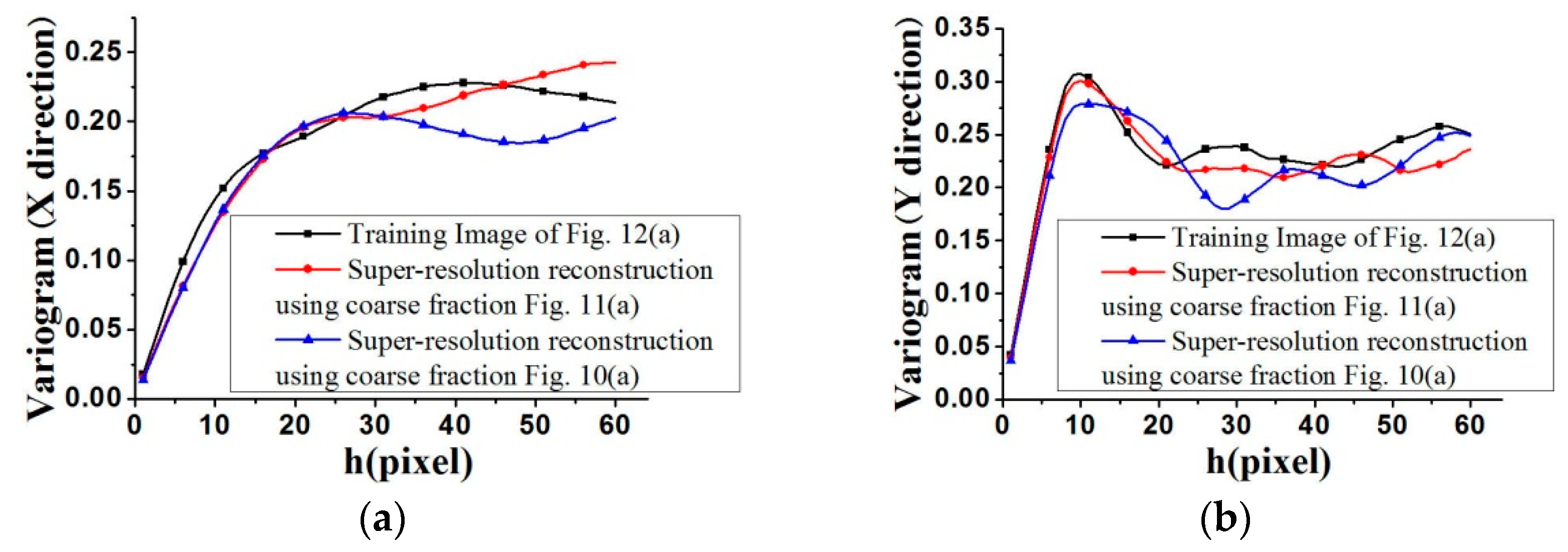
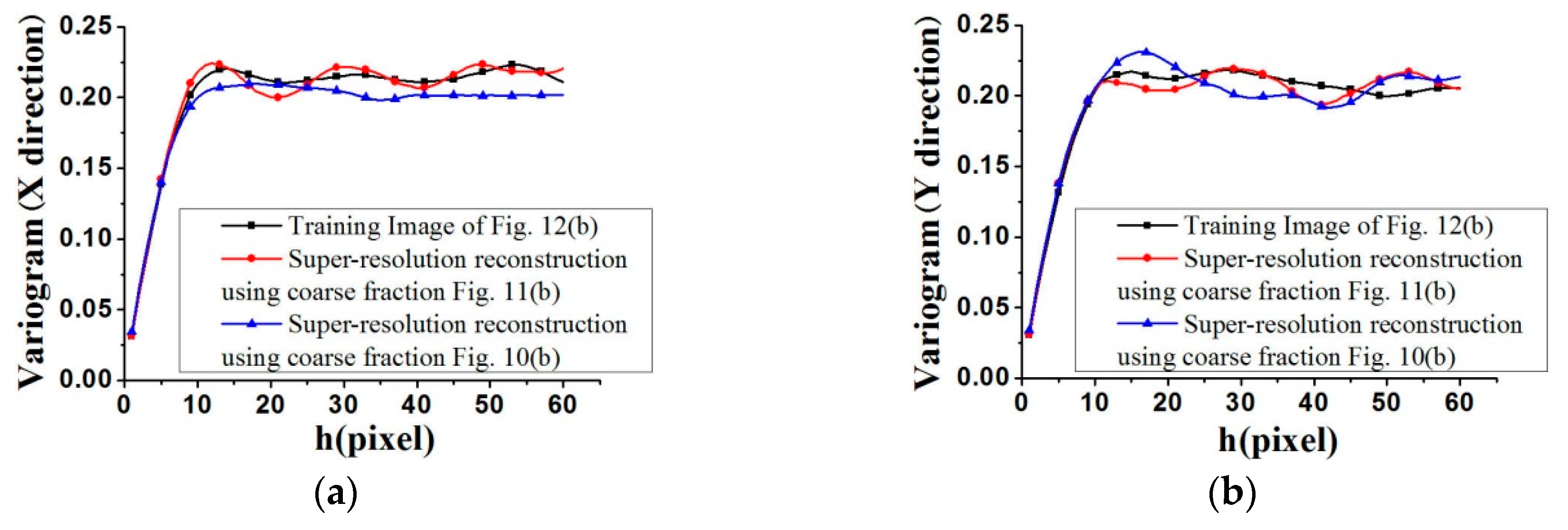
Figure 14 fits the reference image better, by observing their distribution around the 45° line. Another measure of spatial statistical reproduction by variogram curves is given in
Figure 17 and
Figure 18, where the average variograms calculated from 100 super-resolution realizations for each case are compared with the variograms of corresponding training images, demonstrating that coarse fractions with higher resolution enhance the quality of super-resolution reconstruction.
4.2.2. 2D Continuous Simulation
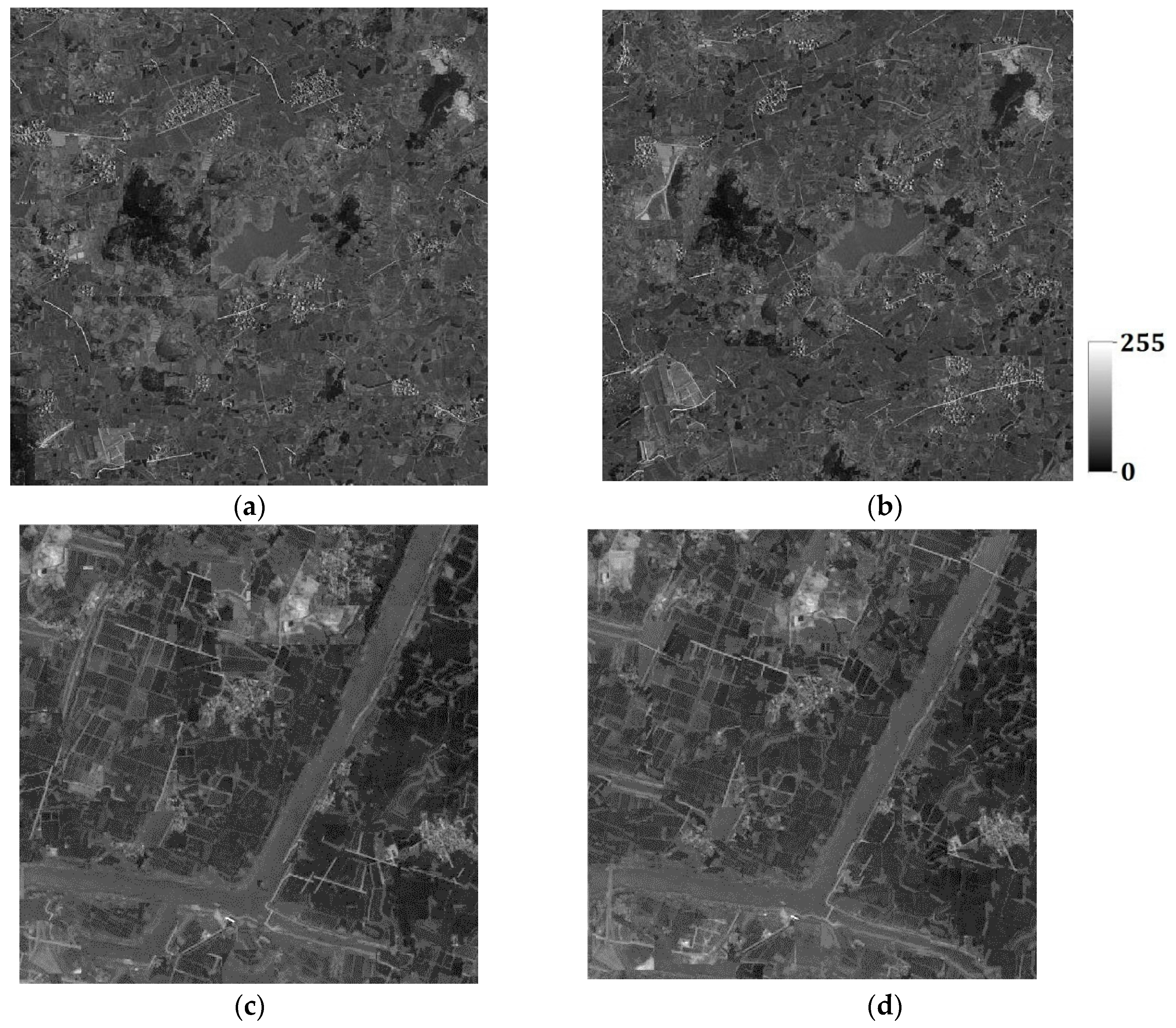
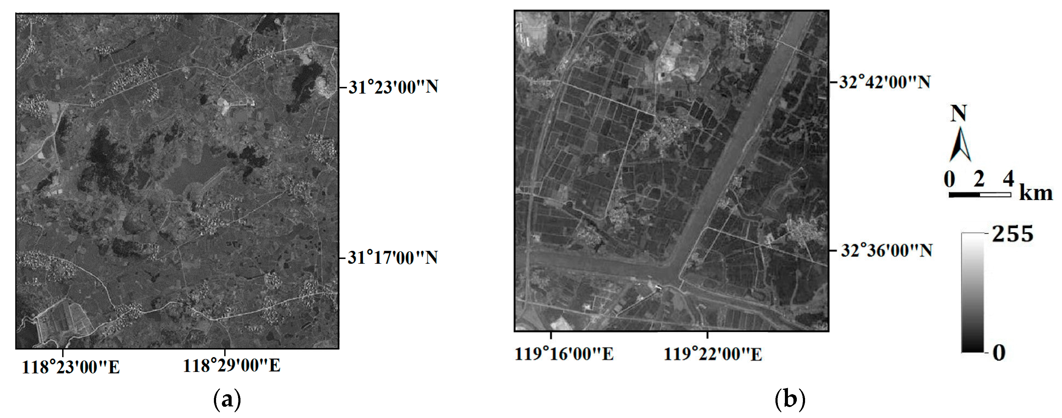
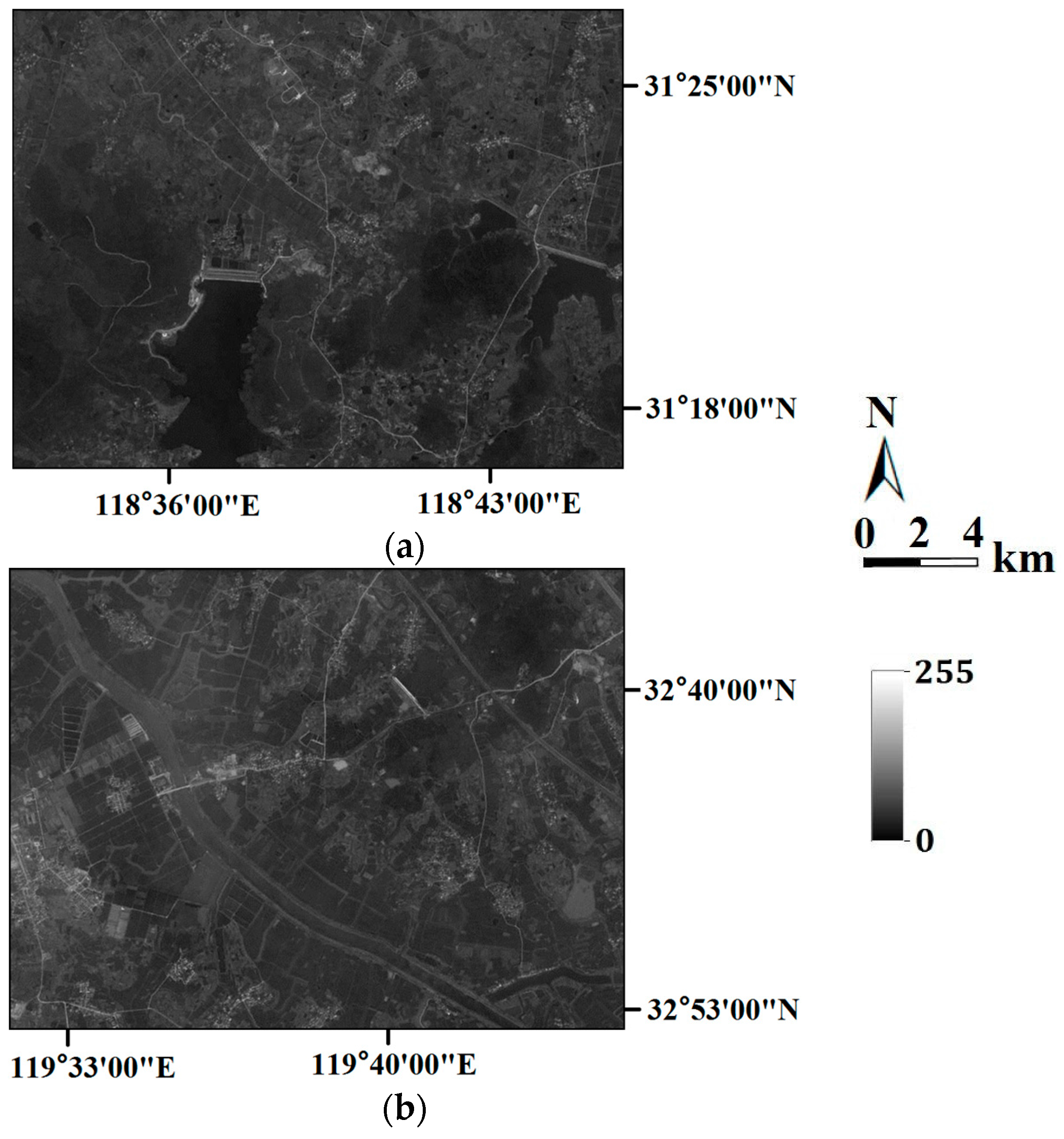
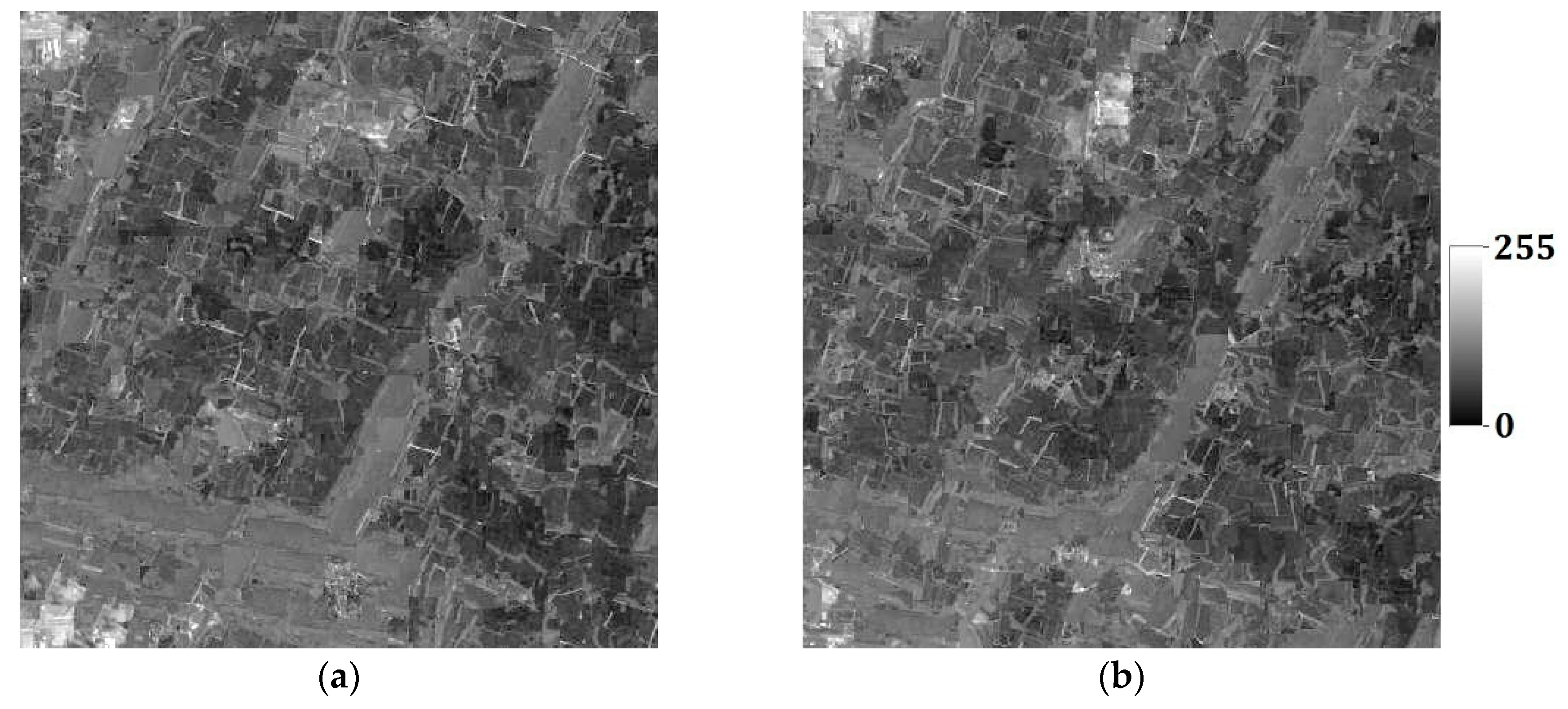
In the last section, the tests are for categorical variables; in what follows, the tests are performed for continuous variables. Consider two remote sensing images as reference images acquired from Landsat TM data (band 2, satellite reflectance values, acquired in June 1996) of an area in the Changjiang River Delta, East China. The reference remote sensing images hereafter called Cases #3 and #4, are shown in
Figure 19. Each image includes 512 × 512 fine resolution pixels, with each pixel of dimension 30 m × 30 m. It is seen that Case #3 contains some scattered forests (deep-colored region), a lake in the center of image, and some farmlands at the left-bottom corner; Case #4 has many rural rectangular farmlands, and a river with two branches crossing the whole image. Both cases have some continuous roads. These typical landmarks in Cases #3 and #4 will be used to evaluate the reconstruction quality.
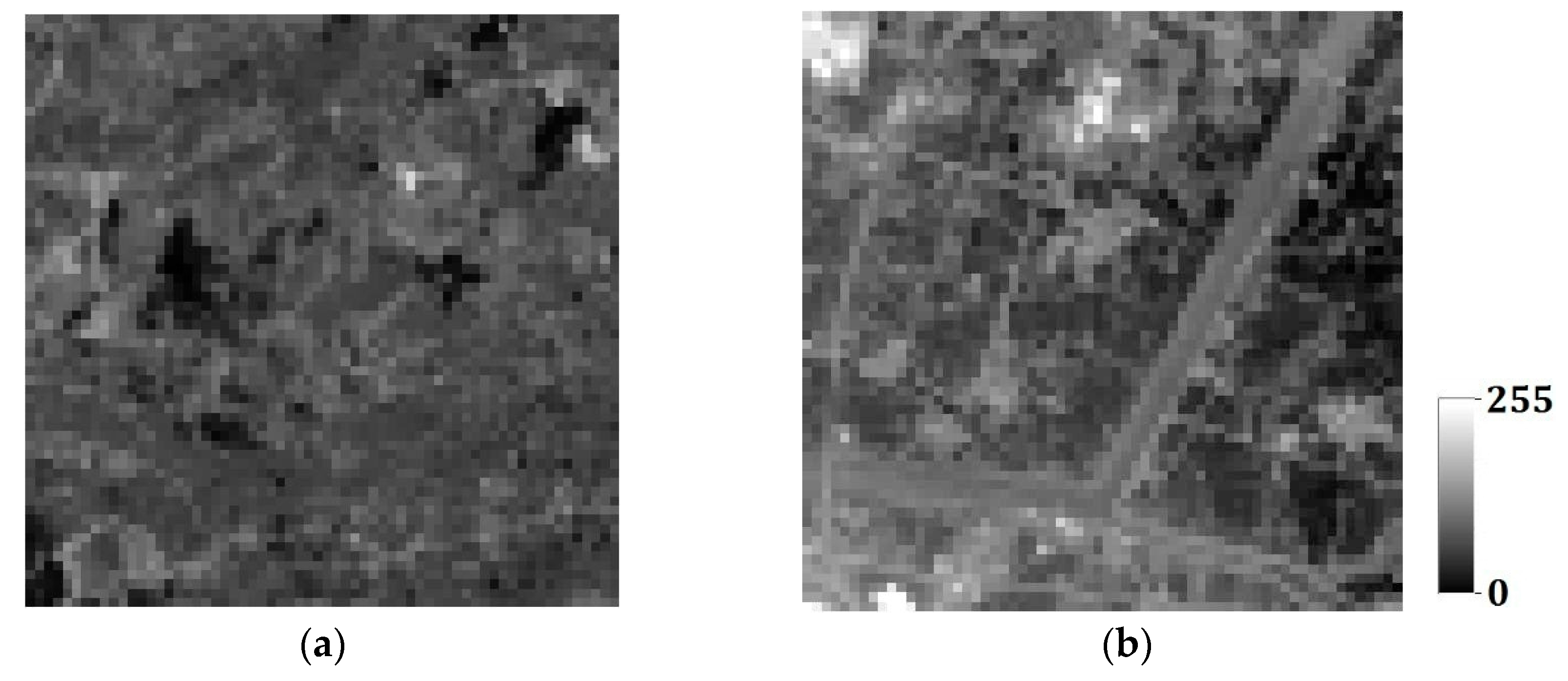
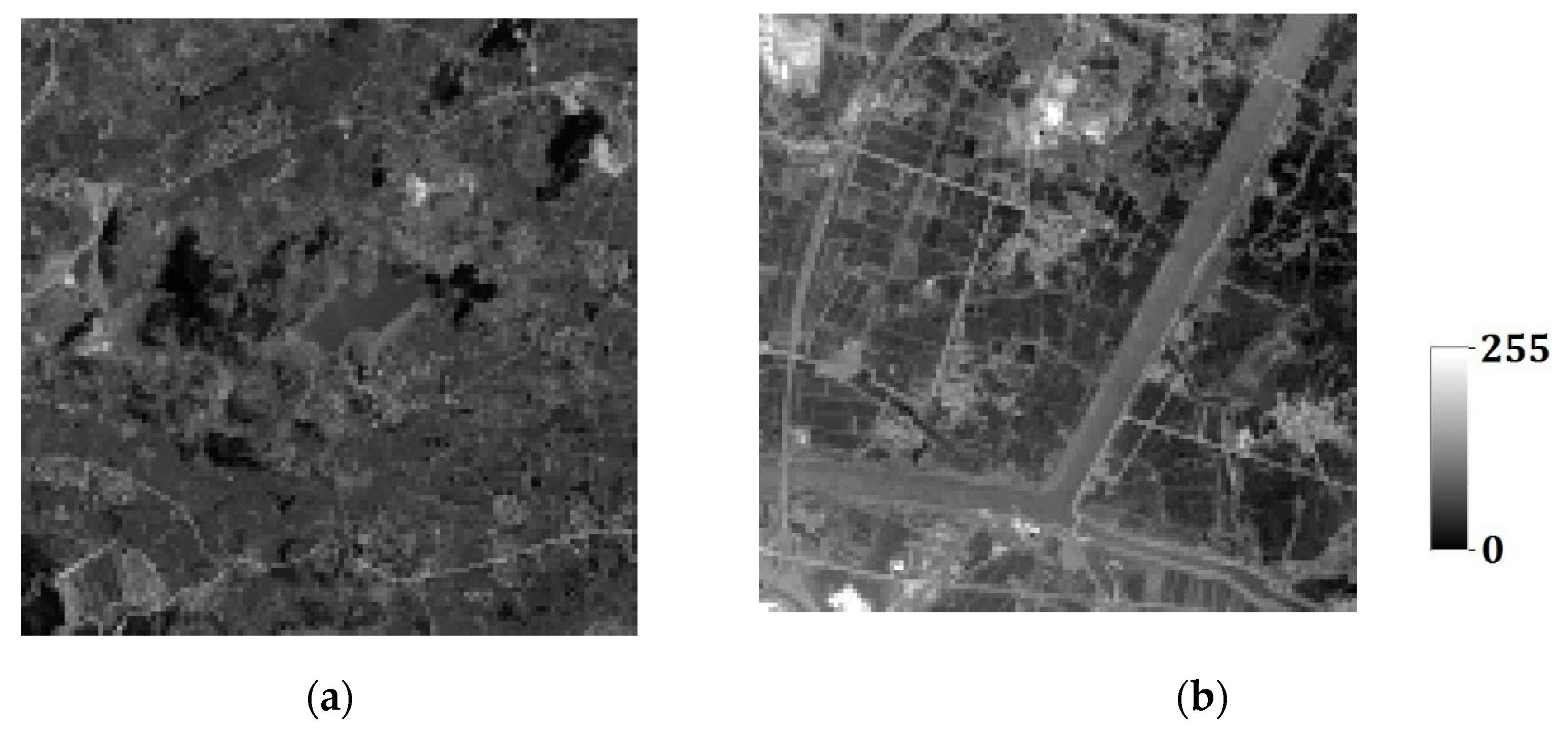
Similar to Cases #1 and #2, the above reference images were then upscaled into two coarse fraction images using two different resolutions by computing the linear average of the fine pixel values within a coarse pixel. The coarse fraction images for Cases #3 and #4, with different resolutions, are shown in
Figure 20 and
Figure 21, respectively. The coarse fraction images in
Figure 20 were computed by linearly averaging the reference images into blocks of 8 × 8 fine pixels each, creating images of 64 × 64 coarse pixels.
Figure 21 is composed of linear averages of Cases #3 and #4, with blocks of 4 × 4 fine pixels each, creating images of 128 × 128 coarse pixels. Obviously, from
Figure 20 to
Figure 21, each coarse pixel is retrogressively comprised of 8 × 8 = 64, and 4 × 4 = 16 fine pixels, and the whole image is progressively comprised of 64 × 64 = 4096 and 128 × 128 = 16,384 coarse pixels.
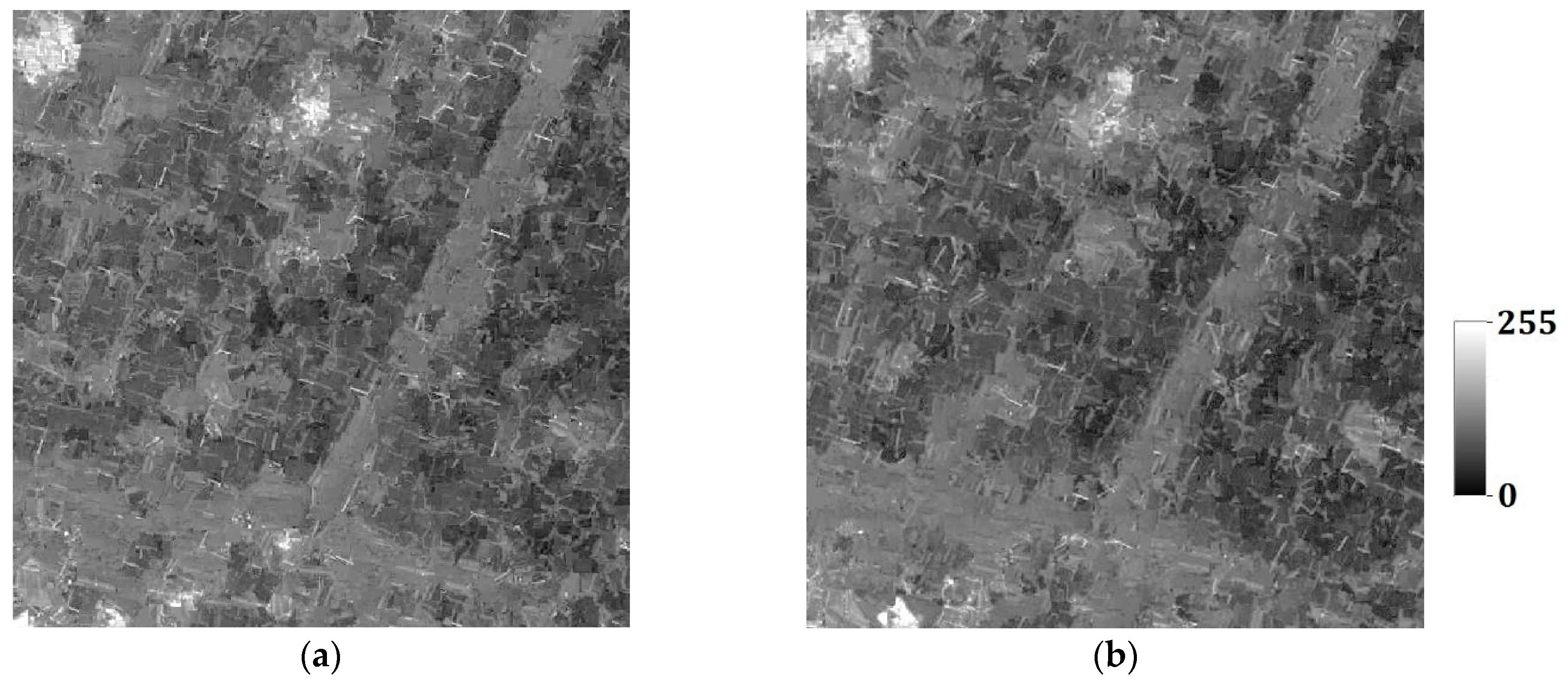
Two training images of 800 × 600 pixels also acquired from Landsat TM data (band 2, satellite reflectance values, acquired in June 1996), are assigned to the two cases of
Figure 19, respectively. Although the training images and reference images are not identical, they have some similar patterns, especially the previously mentioned landmarks, e.g., the lakes, forests, farmlands, rivers and roads can be observed in the training images. In the following reconstruction,
Figure 20a and
Figure 21a with two different coarse resolutions (64 × 64 and 128 × 128 coarse pixels) were used as soft data, respectively, for Case #3, to reproduce the super-resolution reconstructed images; their corresponding training image was
Figure 22a.
Figure 20b and
Figure 21b with two coarse resolutions (64 × 64 and 128 × 128 coarse pixels) were used as soft information, respectively, for the super-resolution reconstruction of Case #4, and accordingly,
Figure 22b was the training image.
The lower dimension
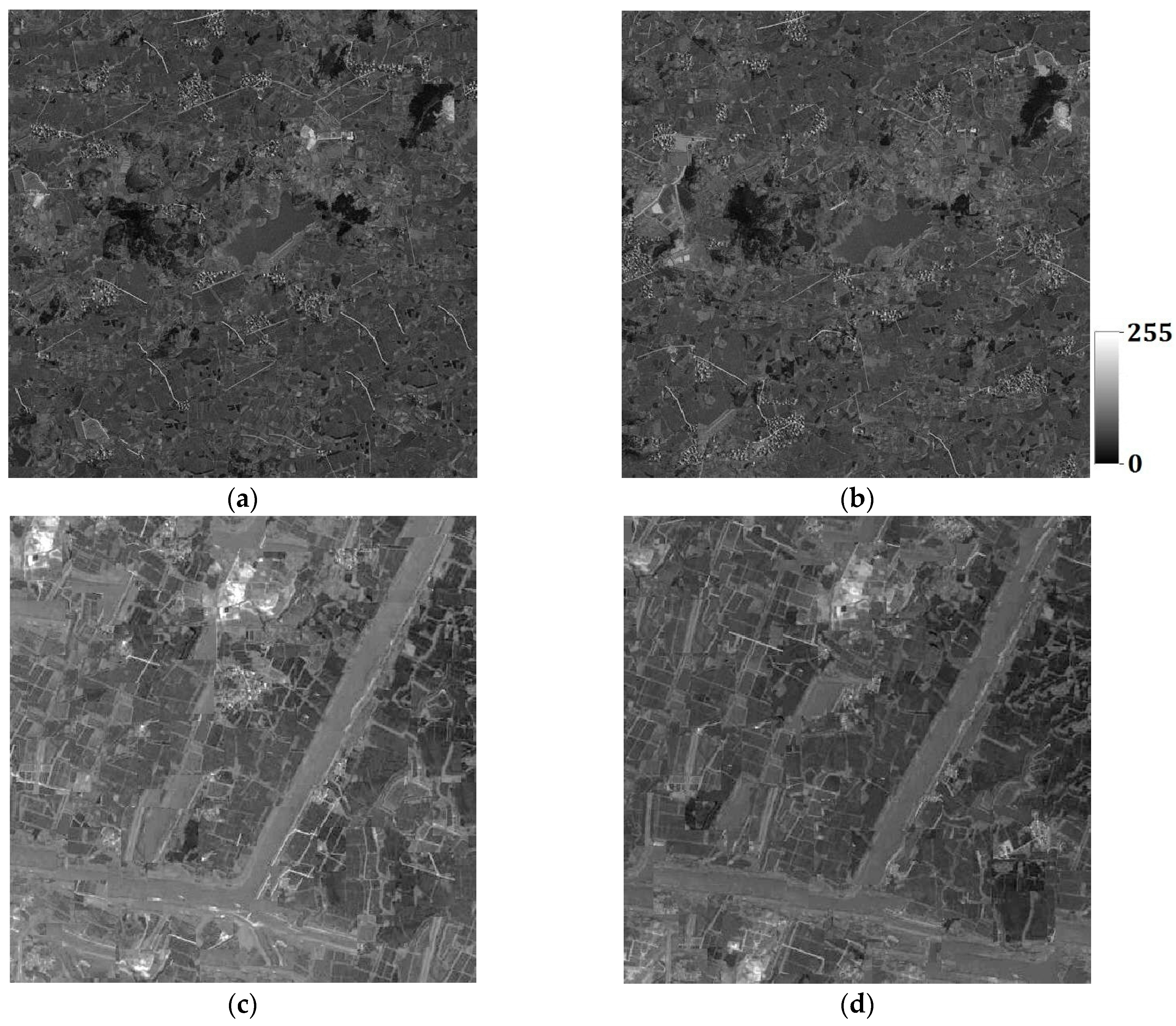
d is set to 4 for both Case #3 and Case #4, derived by the maximum likelihood method. One hundred super-resolution realizations for Cases #3 and #4 were respectively generated with different coarse fractions, and some of them are shown in
Figure 23a–d and
Figure 24a–d. It is clearly seen that the images generated using higher-resolution coarse fraction images (i.e.,
Figure 21a,b) have better reconstruction quality. For example, in
Figure 24a,b, the left-bottom farmlands can still be clearly observed, but almost disappear in
Figure 23a,b; the rivers are more complete in
Figure 24c,d than in
Figure 23c,d, especially the right-bottom part of rivers. However, in all reconstructed images, the roads are heavily disconnected, or not reproduced, because the prior information of roads in the training images is not quite adequate for reconstruction. After all, there are only a small number of roads in the training images.
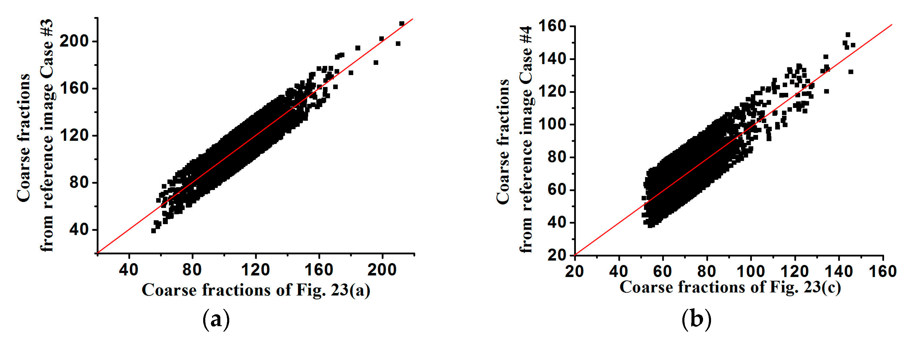
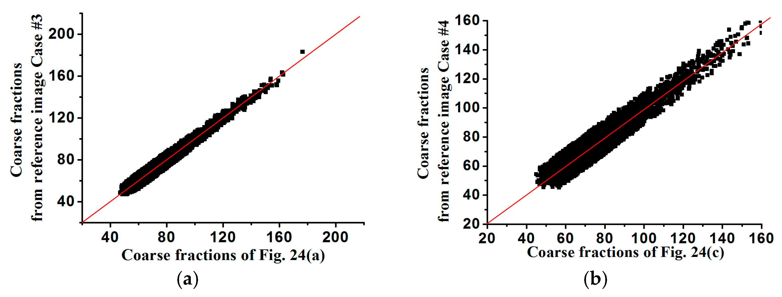
In
Figure 25 and
Figure 26, the averages of coarse fraction images computed from the super-resolution reconstructed images are plotted against the coarse fraction data of reference images, showing the better reproductivity of super-resolution reconstructed results using higher-resolution coarse fractions. In
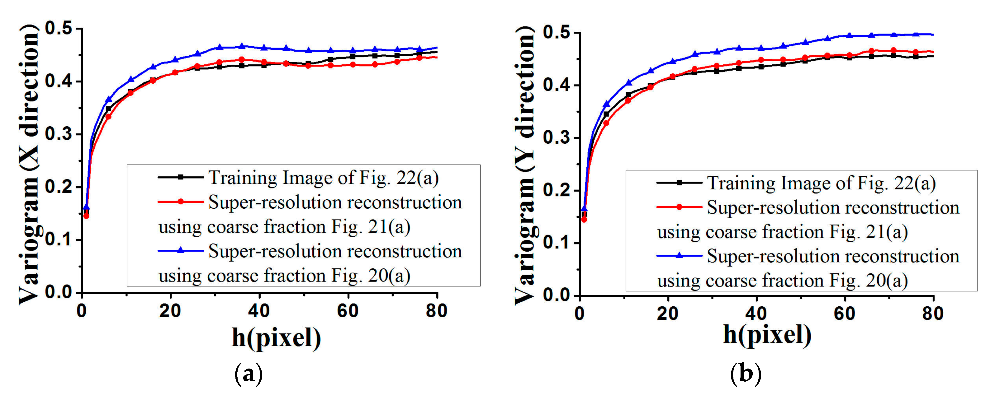
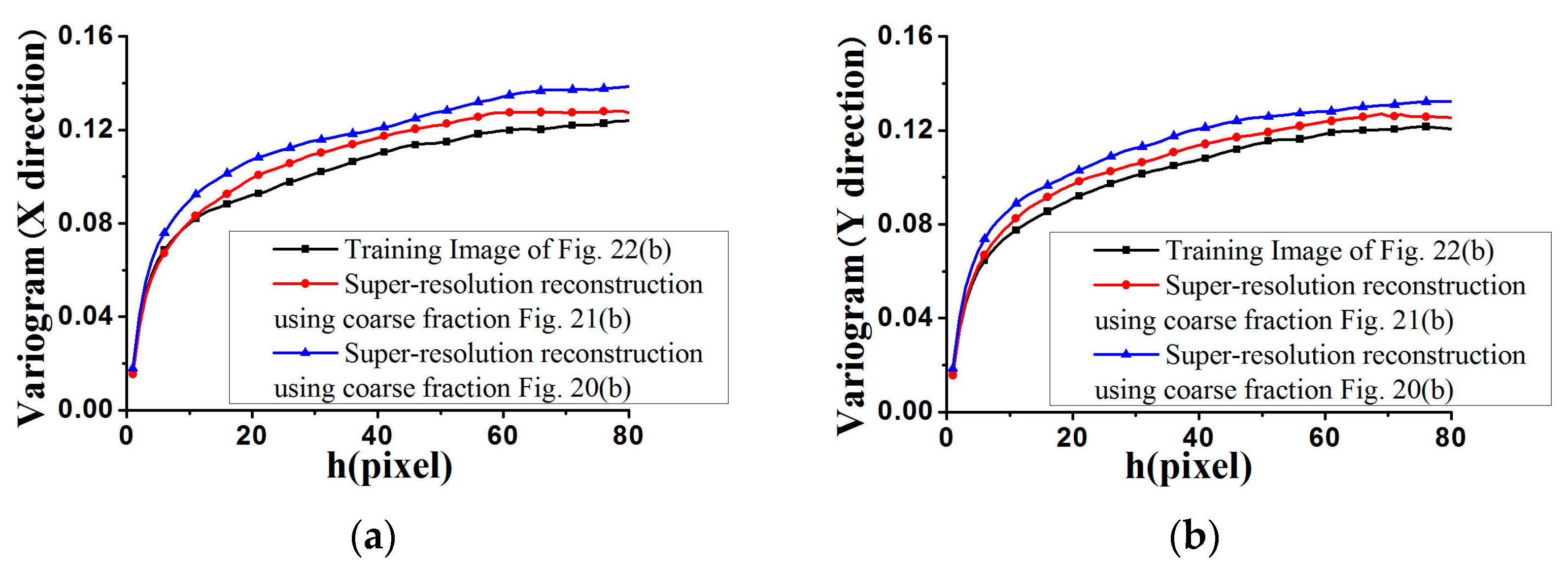
Figure 27 and
Figure 28, the average standardized variograms calculated from 100 super-resolution realizations for Cases #3 and #4 are compared with the standardized variograms of corresponding training images, also demonstrating that coarse fractions with higher resolution enhance the reconstruction quality.
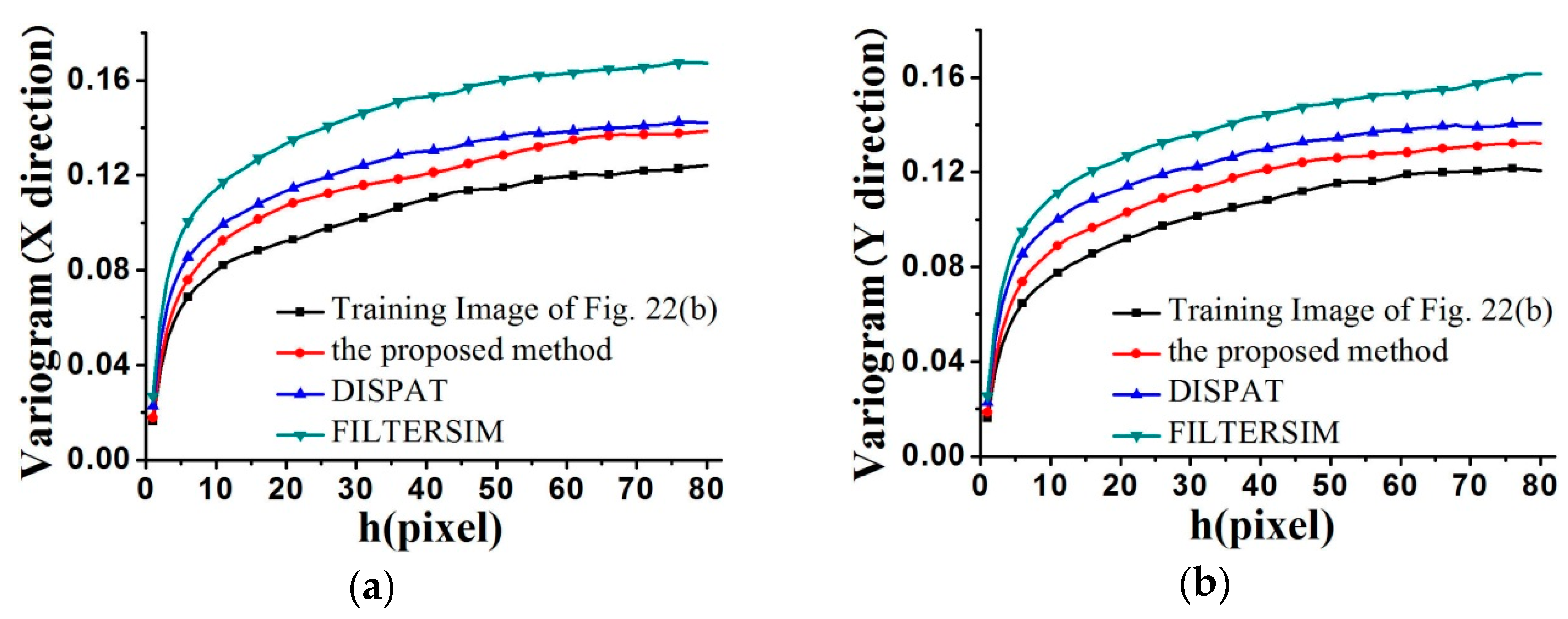
4.3. Results of FILTERSIM and DISPAT
As mentioned previously, FILTERSIM and DISPAT are two typical MPS methods heavily depended upon for linear dimensionality reduction [
23,
24]. To compare them with our method, some tests were performed using FILTERSIM and DISPAT to achieve super-resolution reconstruction, based on the training image of
Figure 22b, and coarse fraction data of
Figure 20b. The low dimensionality of FILTERSIM, and that of DISPAT, are both 6. One hundred reconstructions by FILTERSIM and DISPAT were achieved, and some of them are shown in
Figure 29 and
Figure 30. The standardized variograms are shown in
Figure 31. The simulation time, and maximum memory, are displayed in
Table 1. Clearly, the proposed method has shown its advantage over FILTERSIM and DISPAT in reconstruction quality and CPU time, but the memory costs are quite similar for the three methods.
4.4. Discussion for the Results of the Proposed Method, FILTERSIM, and DISPAT
Theoretically, a higher dimensionality makes classification easier, but uses more time. Recall that the low dimensionality for both FILTERSIM and DISPAT is 6, and that of the proposed method is 4. Hence, it is expected that FILTERSIM and DISPAT use more time, but with better performance in reconstruction quality, which does not accord with the fact that the proposed method has better reconstruction quality and is faster.
The reasons are as follows. First, the data with lower dimensionality helps k-means (both used in the above three methods for the classification of patterns) partition the acquired patterns better than those with higher dimensionality. Second, the time complexity of k-means is O(Npatkclst), where Npat is the number of patterns, kcls is the number of clusters, and t is the iterative time. Data with lower dimensionality leads to less computational time in clustering, as they are associated with fewer iterations in k-means, meaning a smaller t for the proposed method. Finally, ISOMAP has its advantage over the linear dimensionality-reduction methods used in FILTERSIM and DISPAT (i.e., the filters in FILTERSIM and MDS in DISPAT) to achieve better low-dimensional results characterizing the intrinsic features of patterns, leading to better classification.
5. Conclusions
Missing or partial spatial data causes the uncertainty and multiple possible results for super-resolution reconstruction of remote sensing images. Super-resolution reconstruction can be viewed as an under-determined problem when reconstructing a fine resolution image from a set of coarse fractions. Prior structural information can be invoked to reduce or constrain the inherent ambiguity in the super-resolution reconstruction. In this paper, the prior information is extracted by collecting the patterns from training images.
MPS is one of the typical methods for stochastic reconstruction, which can extract the intrinsic features in training images, and export them to the simulated regions. Some classical MPS methods, based on linear dimensionality reduction, can hopefully reduce the dimensionality of patterns in high-dimensional space, to shorten simulation time and raise simulation quality, but their congenital linear essence has limited the application for nonlinear data that are widely existent in the real world. Therefore, in our method, ISOMAP (being a classical nonlinear method for dimensionality reduction) is introduced to achieve nonlinear dimensionality reduction, and combined with MPS to address the above issue. A clustering algorithm is performed to classify these patterns after dimensionality reduction. Afterwards, a reconstruction procedure is designed to sequentially reproduce the features of the training images.
In our method, there are in total, two types of simulation, depending on the available conditional data: (1) the simulation conditioned to soft data, (2) the simulation conditioned to both soft data and hard data. Coarse fraction information from low-resolution remote sensing images that share the intrinsic characteristics with the training images is viewed as soft data, and always present, but initially there is no available hard data. Further, the whole reconstruction turns into being conditioned to both soft data and hard data, with the increase of simulated pixels. Four case studies demonstrate the validity of our method for the super-resolution reconstruction of remote sensing images, including two binary categorical cases, and two continuous cases. Also, our method has shown its advantage over typical MPS methods (i.e., FILTERSIM and DISPAT) using the linear methods of dimensionality reduction. The tests using both finer-resolution and coarser-resolution coarse fraction data prove the former helps to enhance the reconstruction quality better.
At last, note that reconstructing a super-resolution remote sensing image is often not the ultimate aim, because super-resolution images usually are used as input data, at the fine resolution required by detailed spatial analysis operations and decision support systems, which need to investigate the uncertainty related to the super-resolution remote sensing images. The methodology presented in this paper for generating multiple possible super-resolution remote sensing images, can be used towards such an uncertainty assessment for above operations. Our method can also hopefully be used for general super-resolution image reconstruction to recreate a high-resolution image from low-resolution images, which will be studied in our future work.


