Object-Based Classification of Grasslands from High Resolution Satellite Image Time Series Using Gaussian Mean Map Kernels


Abstract
:
1. Introduction
2. Materials
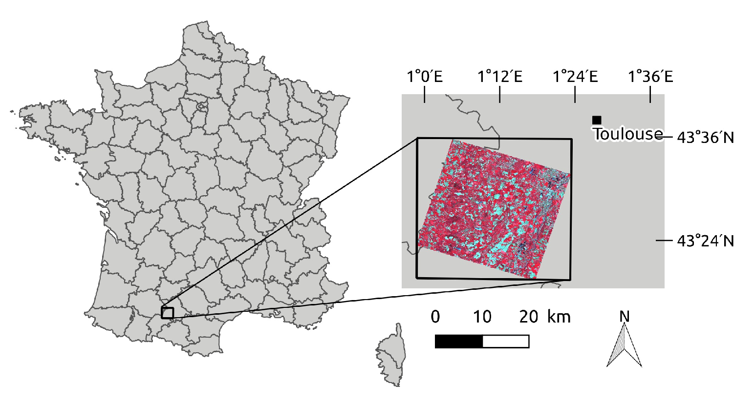
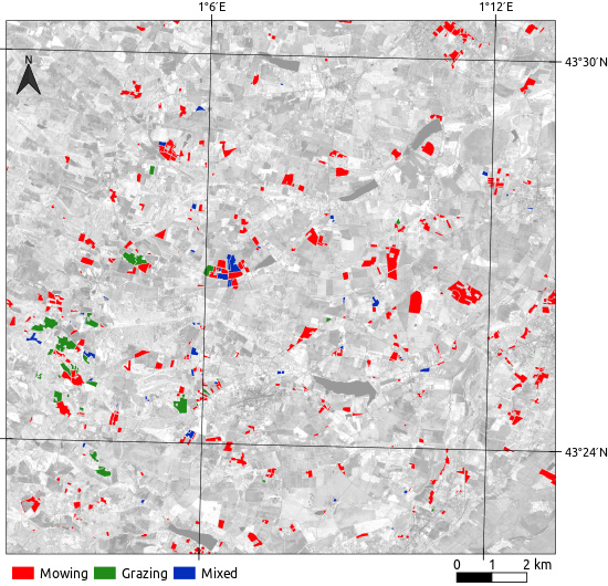
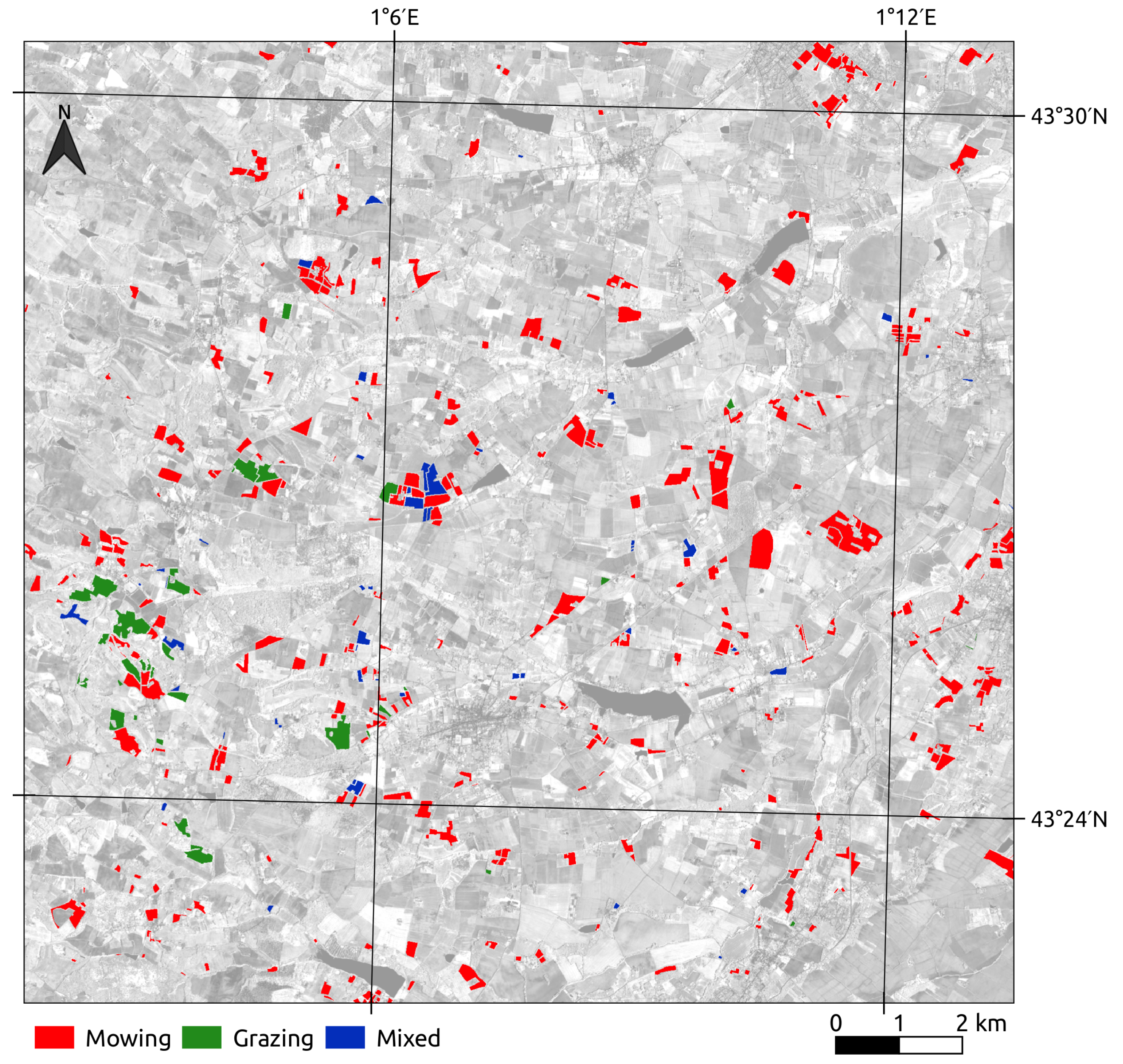
2.1. Study Site
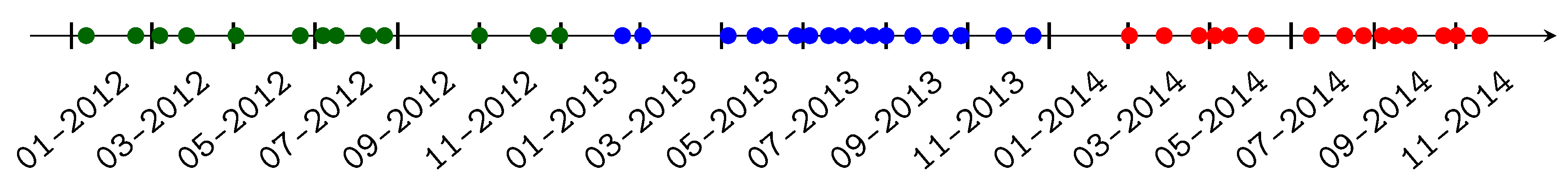
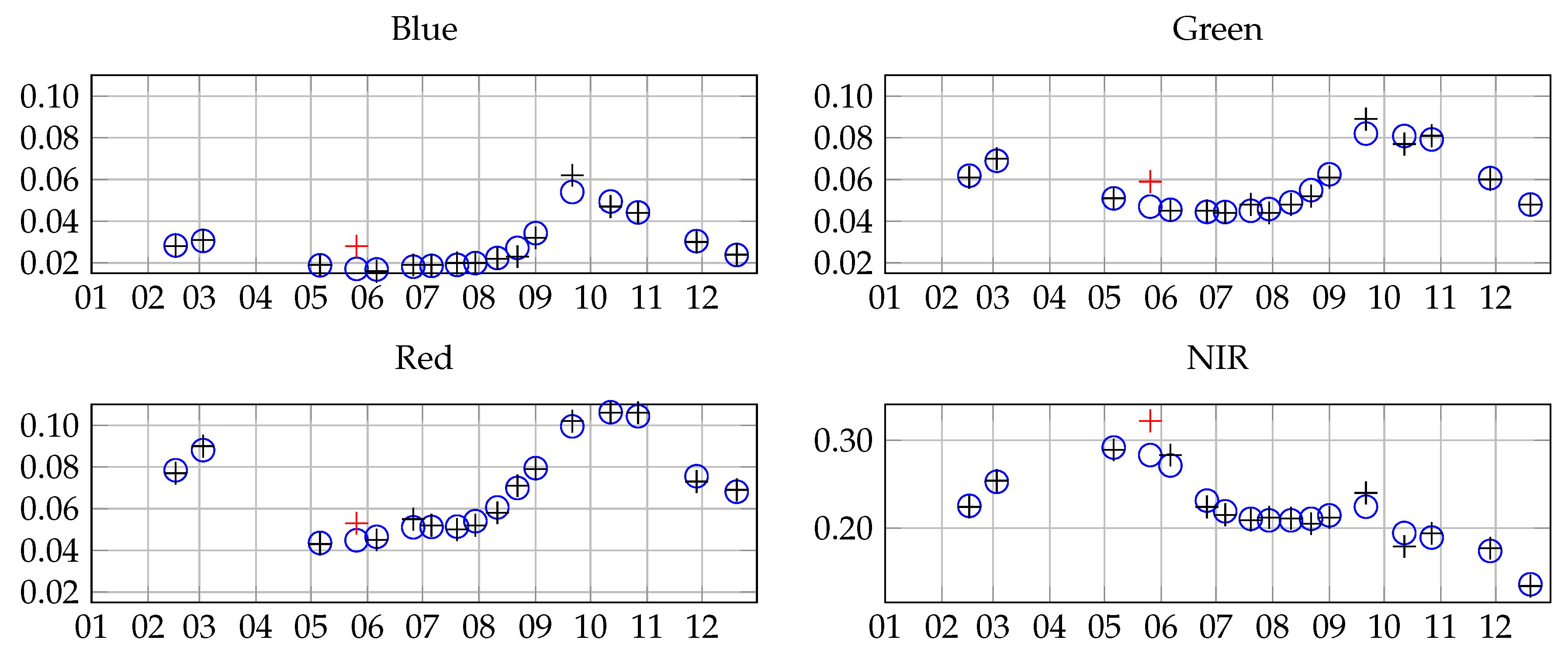
2.2. Satellite Data
2.3. Reference Data
2.3.1. Old and Young Grasslands
2.3.2. Management Practices
3. Methods
3.1. Grassland Modeling
3.1.1. Pixel Level
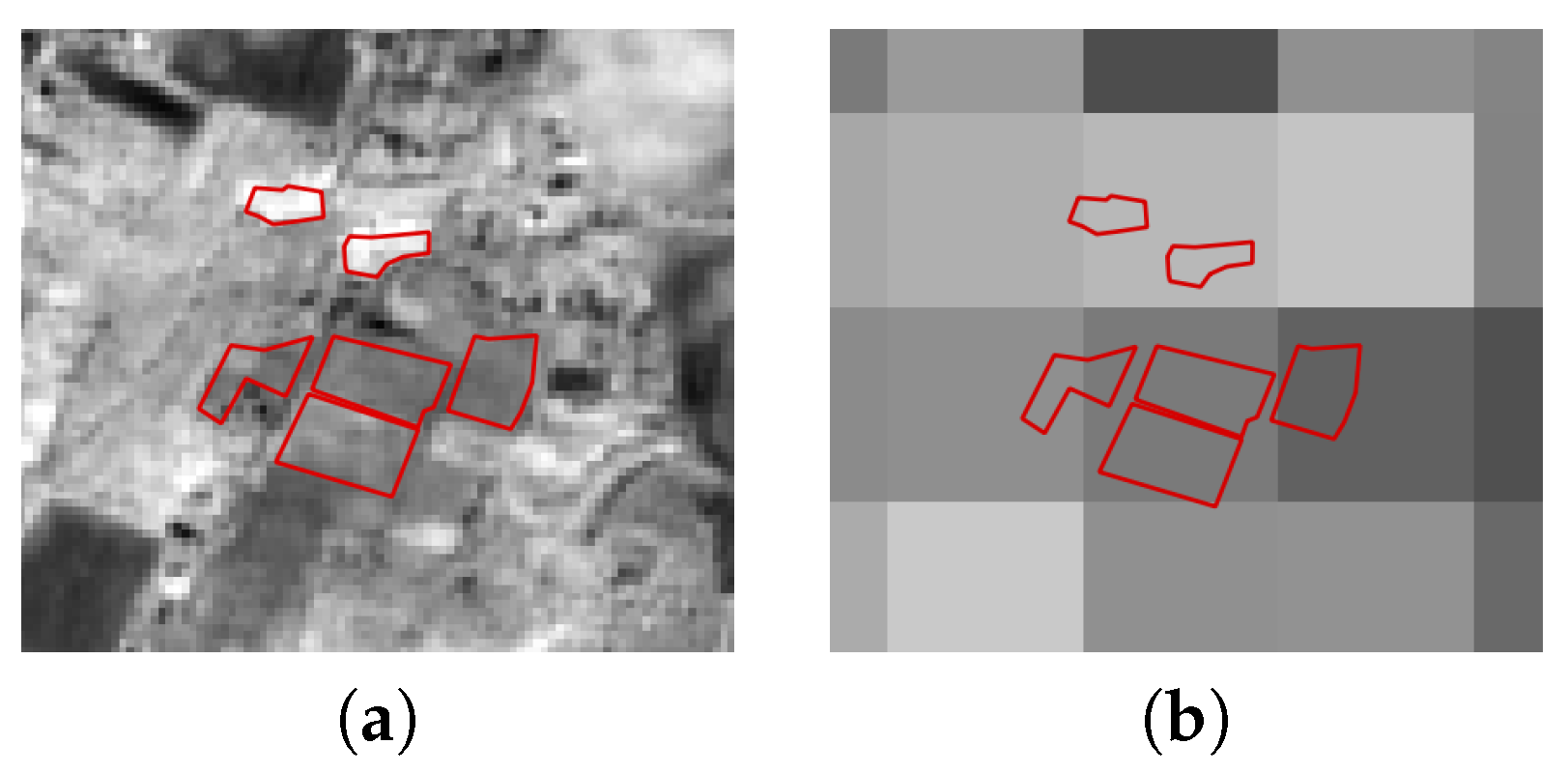
3.1.2. Object Level
3.2. Similarity Measure
3.2.1. Similarity Measure between Distributions
3.2.2. Mean Map Kernels between Distributions
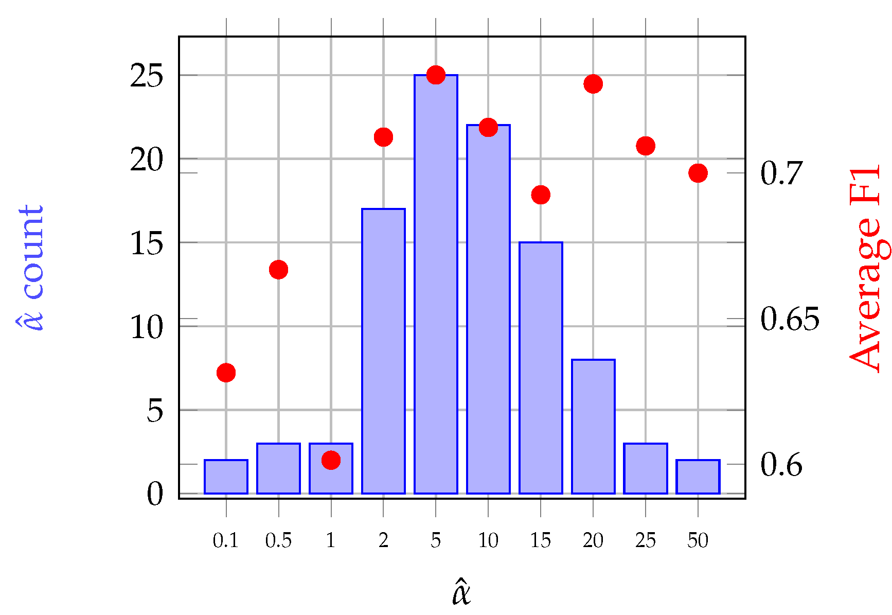
3.2.3. -Gaussian Mean Kernel
- : In this case, Equation (8) reduces to the Gaussian kernel between the mean vectors. It becomes therefore equivalent to an object modeling where only the mean is considered.
- : It corresponds to the Gaussian mean kernel defined in Equation (6).
- : We get a distance, which works only on the covariance matrices. It is therefore equivalent to an object modeling where only the covariance is considered.
- and : The -Gaussian mean kernel simplifies to an RBF kernel built with the Bhattacharyya distance computed between and .
- Whether the heterogeneity of the object is relevant or not,
- Whether the ratio between the number of pixels and the number of variables is high or low.
4. Experiments on Grasslands’ Classification
4.1. Competitive Methods
4.1.1. Pixel-Based and Mean Modeling
- PMV (Pixel Majority Vote): The pixel-based method was described in Section 3.1.1. It classifies each pixel with no a priori information on the object to which the pixel belongs. In order to compare to other object level methods, one class label is extracted per grassland by a majority vote done among the pixels belonging to the same grassland.
- (mean): The distribution of the pixels reflectance of is modeled by its mean vector (see Section 3.1.2).
4.1.2. Divergence Methods
- HDKLD (High Dimensional Kullback–Leibler Divergence): This method uses the Kullback–Leibler divergence for Gaussian distributions with a regularization on covariance matrices such as described in [82].
- BD (Bhattacharyya Distance): This method uses the Bhattacharyya distance in the case of Gaussian distributions:Small eigenvalues of the covariance matrices are shrinked to the value to make the computation tractable [83].
4.1.3. Mean Map Kernel-Based Methods
- EMK (Empirical Mean Kernel): This method uses the empirical mean map kernel of Equation (3) and it is pixel-based.
- GMK (Gaussian Mean Kernel): This method is based on the normalized Gaussian mean kernel (Equation (6)).
- GMK (-Gaussian Mean Kernel): This method is based on the proposed normalized -Gaussian mean kernel (Equation (8)).
4.2. Classification Protocol
4.3. Results
4.3.1. Old and Young Grasslands: Inter-Annual Time Series
4.3.2. Management Practices: Intra-Annual Time Series
4.4. Discussion
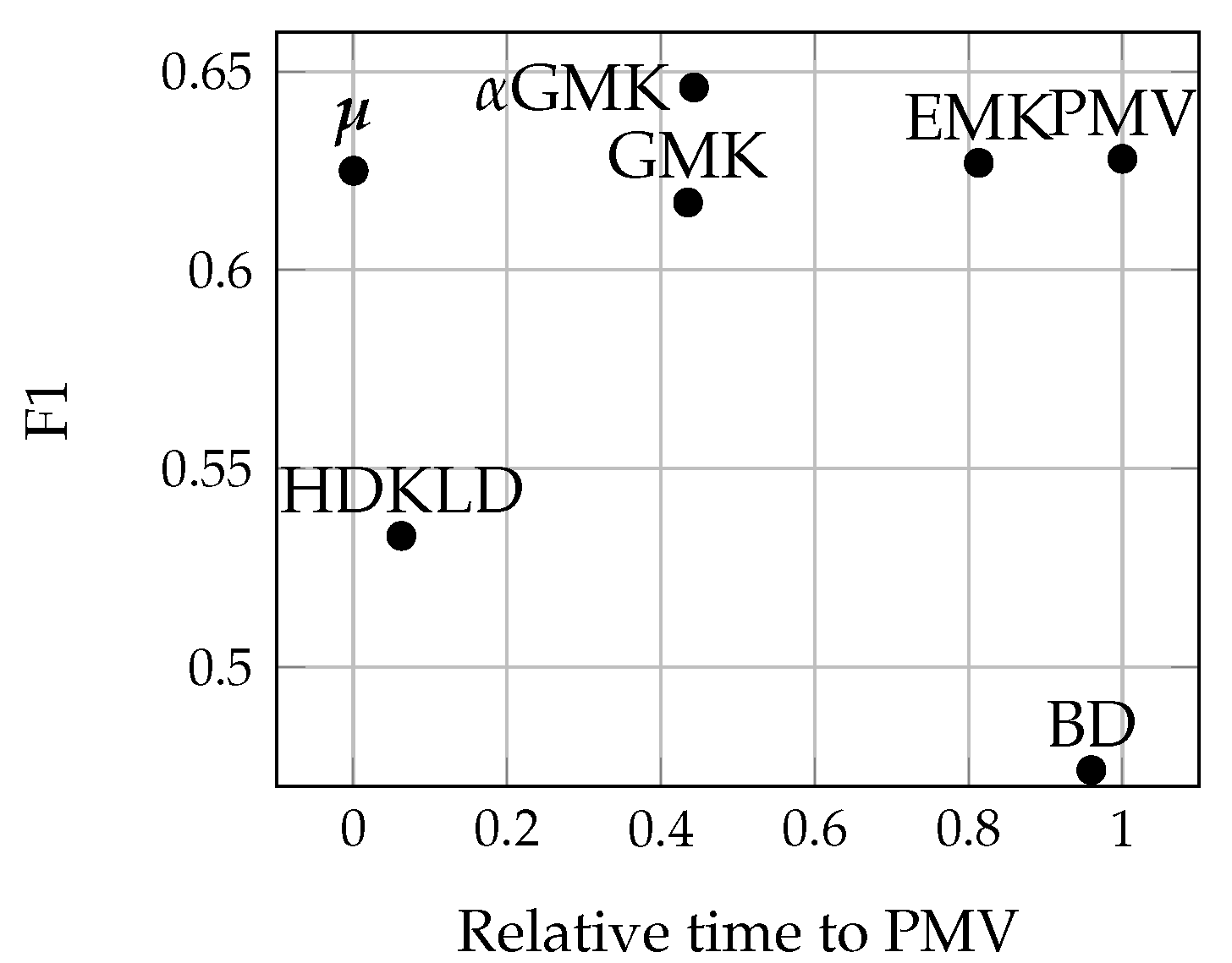
4.4.1. Methods’ Efficiency
4.4.2. Grassland Modeling
4.4.3. Acquisition Dates
4.4.4. Grassland Typology
4.4.5. Comparison with Existing Works
4.5. Prediction of Management Practices on the Land Use Database Grasslands
5. Conclusions
Supplementary Materials
Acknowledgments
Author Contributions
Conflicts of Interest
Abbreviations
| BD | Bhattacharyya Distance |
| EMK | Empirical Mean Kernel |
| GIS | Geographic Information System |
| GMK | Gaussian Mean Kernel |
| HDKLD | High Dimensional Kullback–Leibler Divergence |
| JMD | Jeffries-Matusita Distance |
| KLD | Kullback–Leibler Divergence |
| LAI | Leaf Area Index |
| NDVI | Normalized Difference Vegetation Index |
| NIR | Near Infrared |
| PMV | Pixel Majority Vote |
| RBF | Radial Basis Function |
| SITS | Satellite Image Time Series |
| SVM | Support Vector Machine |
| GMK | -Gaussian Mean Kernel |
Appendix A
References
- Eriksson, A.; Eriksson, O.; Berglund, H. Species Abundance Patterns of Plants in Swedish Semi-Natural Pastures. Ecography 1995, 18, 310–317. [Google Scholar] [CrossRef]
- Cousins, S.A.; Eriksson, O. The influence of management history and habitat on plant species richness in a rural hemiboreal landscape, Sweden. Landsc. Ecol. 2002, 17, 517–529. [Google Scholar] [CrossRef]
- Gardi, C.; Tomaselli, M.; Parisi, V.; Petraglia, A.; Santini, C. Soil quality indicators and biodiversity in northern Italian permanent grasslands. Eur. J. Soil Biol. 2002, 38, 103–110. [Google Scholar] [CrossRef]
- Critchley, C.; Burke, M.; Stevens, D. Conservation of lowland semi-natural grasslands in the UK: A review of botanical monitoring results from agri-environment schemes. Biol. Conserv. 2004, 115, 263–278. [Google Scholar] [CrossRef]
- Werling, B.P.; Dickson, T.L.; Isaacs, R.; Gaines, H.; Gratton, C.; Gross, K.L.; Liere, H.; Malmstrom, C.M.; Meehan, T.D.; Ruan, L.; et al. Perennial grasslands enhance biodiversity and multiple ecosystem services in bioenergy landscapes. Proc. Natl. Acad. Sci. USA 2014, 111, 1652–1657. [Google Scholar] [CrossRef] [PubMed]
- Austrheim, G.; Olsson, E.G.A. How does continuity in grassland management after ploughing affect plant community patterns? Plant Ecol. 1999, 145, 59–74. [Google Scholar] [CrossRef]
- Norderhaug, A.; Ihse, M.; Pedersen, O. Biotope patterns and abundance of meadow plant species in a Norwegian rural landscape. Landsc. Ecol. 2000, 15, 201–218. [Google Scholar] [CrossRef]
- Waldhardt, R.; Otte, A. Indicators of plant species and community diversity in grasslands. Agric. Ecosyst. Environ. 2003, 98, 339–351. [Google Scholar] [CrossRef]
- Hansson, M.; Fogelfors, H. Management of a semi-natural grassland; results from a 15-year-old experiment in southern Sweden. J. Veg. Sci. 2000, 11, 31–38. [Google Scholar] [CrossRef]
- Moog, D.; Poschlod, P.; Kahmen, S.; Schreiber, K.F. Comparison of species composition between different grassland management treatments after 25 years. Appl. Veg. Sci. 2002, 5, 99–106. [Google Scholar] [CrossRef]
- Zechmeister, H.; Schmitzberger, I.; Steurer, B.; Peterseil, J.; Wrbka, T. The influence of land-use practices and economics on plant species richness in meadows. Biol. Conserv. 2003, 114, 165–177. [Google Scholar] [CrossRef]
- Plantureux, S.; Peeters, A.; McCracken, D. Biodiversity in intensive grasslands: Effect of management, improvement and challenges. Agron. Res. 2005, 3, 153–164. [Google Scholar]
- Muller, S. Appropriate agricultural management practices required to ensure conservation and biodiversity of environmentally sensitive grassland sites designated under Natura 2000. Agric. Ecosyst. Environ. 2002, 89, 261–266. [Google Scholar] [CrossRef]
- Rocchini, D.; Boyd, D.S.; Féret, J.B.; Foody, G.M.; He, K.S.; Lausch, A.; Nagendra, H.; Wegmann, M.; Pettorelli, N. Satellite remote sensing to monitor species diversity: Potential and pitfalls. Remote Sens. Ecol. Conserv. 2016, 2, 25–36. [Google Scholar] [CrossRef]
- Pettorelli, N.; Laurance, W.F.; O’Brien, T.G.; Wegmann, M.; Nagendra, H.; Turner, W. Satellite remote sensing for applied ecologists: Opportunities and challenges. J. Appl. Ecol. 2014, 51, 839–848. [Google Scholar] [CrossRef]
- Newton, A.C.; Hill, R.A.; Echeverría, C.; Golicher, D.; Rey Benayas, J.M.; Cayuela, L.; Hinsley, S.A. Remote sensing and the future of landscape ecology. Prog. Phys. Geogr. 2009, 33, 528–546. [Google Scholar] [CrossRef]
- Gu, Y.; Wylie, B.K.; Bliss, N.B. Mapping grassland productivity with 250-m eMODIS NDVI and SSURGO database over the Greater Platte River Basin, USA. Ecol. Indic. 2013, 24, 31–36. [Google Scholar] [CrossRef]
- Li, Z.; Huffman, T.; McConkey, B.; Townley-Smith, L. Monitoring and modeling spatial and temporal patterns of grassland dynamics using time-series MODIS NDVI with climate and stocking data. Remote Sens. Environ. 2013, 138, 232–244. [Google Scholar] [CrossRef]
- Gu, Y.; Wylie, B.K. Developing a 30-m grassland productivity estimation map for central Nebraska using 250-m MODIS and 30-m Landsat-8 observations. Remote Sens. Environ. 2015, 171, 291–298. [Google Scholar] [CrossRef]
- Friedl, M.A.; Michaelsen, J.; Davis, F.W.; Walker, H.; Schimel, D.S. Estimating grassland biomass and Leaf Area Index using ground and satellite data. Int. J. Remote Sens. 1994, 15, 1401–1420. [Google Scholar] [CrossRef]
- Wylie, B.; Meyer, D.; Tieszen, L.; Mannel, S. Satellite mapping of surface biophysical parameters at the biome scale over the North American grasslands: A case study. Remote Sens. Environ. 2002, 79, 266–278. [Google Scholar] [CrossRef]
- Darvishzadeh, R.; Skidmore, A.; Schlerf, M.; Atzberger, C.; Corsi, F.; Cho, M. LAI and chlorophyll estimation for a heterogeneous grassland using hyperspectral measurements. ISPRS J. Photogramm. Remote Sens. 2008, 63, 409–426. [Google Scholar] [CrossRef]
- He, Y.; Guo, X.; Wilmshurst, J.F. Reflectance measures of grassland biophysical structure. Int. J. Remote Sens. 2009, 30, 2509–2521. [Google Scholar] [CrossRef]
- Asam, S.; Fabritius, H.; Klein, D.; Conrad, C.; Dech, S. Derivation of leaf area index for grassland within alpine upland using multi-temporal RapidEye data. Int. J. Remote Sens. 2013, 34, 8628–8652. [Google Scholar] [CrossRef]
- Schmidtlein, S.; Sassin, J. Mapping of continuous floristic gradients in grasslands using hyperspectral imagery. Remote Sens. Environ. 2004, 92, 126–138. [Google Scholar] [CrossRef]
- Ishii, J.; Lu, S.; Funakoshi, S.; Shimizu, Y.; Omasa, K.; Washitani, I. Mapping potential habitats of threatened plant species in a moist tall grassland using hyperspectral imagery. Biodivers. Conserv. 2009, 18, 2521–2535. [Google Scholar] [CrossRef]
- Fava, F.; Parolo, G.; Colombo, R.; Gusmeroli, F.; Marianna, G.D.; Monteiro, A.; Bocchi, S. Fine-scale assessment of hay meadow productivity and plant diversity in the European Alps using field spectrometric data. Agric. Ecosyst. Environ. 2010, 137, 151–157. [Google Scholar] [CrossRef]
- Oldeland, J.; Wesuls, D.; Rocchini, D.; Schmidt, M.; Jürgens, N. Does using species abundance data improve estimates of species diversity from remotely sensed spectral heterogeneity? Ecol. Indic. 2010, 10, 390–396. [Google Scholar] [CrossRef]
- Feilhauer, H.; Faude, U.; Schmidtlein, S. Combining Isomap ordination and imaging spectroscopy to map continuous floristic gradients in a heterogeneous landscape. Remote Sens. Environ. 2011, 115, 2513–2524. [Google Scholar] [CrossRef]
- Duniway, M.C.; Karl, J.W.; Schrader, S.; Baquera, N.; Herrick, J.E. Rangeland and pasture monitoring: An approach to interpretation of high-resolution imagery focused on observer calibration for repeatability. Environ. Monit. Assess. 2012, 184, 3789–3804. [Google Scholar] [CrossRef] [PubMed]
- Punalekar, S.; Verhoef, A.; Tatarenko, I.V.; van der Tol, C.; Macdonald, D.M.J.; Marchant, B.; Gerard, F.; White, K.; Gowing, D. Characterization of a Highly Biodiverse Floodplain Meadow Using Hyperspectral Remote Sensing within a Plant Functional Trait Framework. Remote Sens. 2016, 8, 112. [Google Scholar] [CrossRef]
- Hilker, T.; Natsagdorj, E.; Waring, R.H.; Lyapustin, A.; Wang, Y. Satellite observed widespread decline in Mongolian grasslands largely due to overgrazing. Glob. Chang. Biol. 2014, 20, 418–428. [Google Scholar] [CrossRef] [PubMed]
- Cao, R.; Chen, J.; Shen, M.; Tang, Y. An improved logistic method for detecting spring vegetation phenology in grasslands from MODIS EVI time-series data. Agric. For. Meteorol. 2015, 200, 9–20. [Google Scholar] [CrossRef]
- Eriksson, O.; Cousins, S.A.; Bruun, H.H. Land-use history and fragmentation of traditionally managed grasslands in Scandinavia. J. Veg. Sci. 2002, 13, 743–748. [Google Scholar] [CrossRef]
- Zillmann, E.; Gonzalez, A.; Herrero, E.J.M.; van Wolvelaer, J.; Esch, T.; Keil, M.; Weichelt, H.; Garzón, A.M. Pan-European Grassland Mapping Using Seasonal Statistics From Multisensor Image Time Series. IEEE J. Sel. Top. Appl. Earth Obs. Remote Sens. 2014, 7, 3461–3472. [Google Scholar] [CrossRef]
- Ali, I.; Cawkwell, F.; Dwyer, E.; Barrett, B.; Green, S. Satellite remote sensing of grasslands: From observation to management. J. Plant Ecol. 2016, 9, 649–671. [Google Scholar] [CrossRef]
- Nagendra, H. Using remote sensing to assess biodiversity. Int. J. Remote Sens. 2001, 22, 2377–2400. [Google Scholar] [CrossRef]
- Blaschke, T.; Hay, G.J.; Kelly, M.; Lang, S.; Hofmann, P.; Addink, E.; Feitosa, R.Q.; van der Meer, F.; van der Werff, H.; van Coillie, F.; Tiede, D. Geographic Object-Based Image Analysis—Towards a new paradigm. ISPRS J. Photogramm. Remote Sens. 2014, 87, 180–191. [Google Scholar] [CrossRef] [PubMed]
- Poças, I.; Cunha, M.; Pereira, L.S. Dynamics of mountain semi-natural grassland meadows inferred from SPOT-VEGETATION and field spectroradiometer data. Int. J. Remote Sens. 2012, 33, 4334–4355. [Google Scholar] [CrossRef]
- Halabuk, A.; Mojses, M.; Halabuk, M.; David, S. Towards Detection of Cutting in Hay Meadows by Using of NDVI and EVI Time Series. Remote Sens. 2015, 7, 6107–6132. [Google Scholar] [CrossRef]
- Lucas, R.; Rowlands, A.; Brown, A.; Keyworth, S.; Bunting, P. Rule-based classification of multi-temporal satellite imagery for habitat and agricultural land cover mapping. ISPRS J. Photogramm. Remote Sens. 2007, 62, 165–185. [Google Scholar] [CrossRef]
- Toivonen, T.; Luoto, M. Landsat TM images in mapping of semi-natural grasslands and analysing of habitat pattern in an agricultural landscape in south-west Finland. FENNIA Int. J. Geogr. 2003, 181, 49–67. [Google Scholar]
- Nagendra, H.; Lucas, R.; Honrado, J.P.; Jongman, R.H.; Tarantino, C.; Adamo, M.; Mairota, P. Remote sensing for conservation monitoring: Assessing protected areas, habitat extent, habitat condition, species diversity, and threats. Ecol. Indic. 2013, 33, 45–59. [Google Scholar] [CrossRef]
- Price, K.P.; Guo, X.; Stiles, J.M. Optimal Landsat TM band combinations and vegetation indices for discrimination of six grassland types in eastern Kansas. Int. J. Remote Sens. 2002, 23, 5031–5042. [Google Scholar] [CrossRef]
- Gamon, J.A.; Field, C.B.; Roberts, D.A.; Ustin, S.L.; Valentini, R. Airbone Imaging Spectrometry Functional patterns in an annual grassland during an AVIRIS overflight. Remote Sens. Environ. 1993, 44, 239–253. [Google Scholar] [CrossRef]
- Corbane, C.; Lang, S.; Pipkins, K.; Alleaume, S.; Deshayes, M.; Millán, V.E.G.; Strasser, T.; Borre, J.V.; Toon, S.; Michael, F. Remote sensing for mapping natural habitats and their conservation status—New opportunities and challenges. Int. J. Appl. Earth Obs. Geoinf. 2015, 37, 7–16. [Google Scholar] [CrossRef]
- Wulder, M.A.; Hall, R.J.; Coops, N.C.; Franklin, S.E. High Spatial Resolution Remotely Sensed Data for Ecosystem Characterization. BioScience 2004, 54, 511–521. [Google Scholar] [CrossRef]
- Buck, O.; Millán, V.E.G.; Klink, A.; Pakzad, K. Using information layers for mapping grassland habitat distribution at local to regional scales. Int. J. Appl. Earth Obs. Geoinf. 2015, 37, 83–89. [Google Scholar] [CrossRef]
- Franke, J.; Keuck, V.; Siegert, F. Assessment of grassland use intensity by remote sensing to support conservation schemes. J. Nat. Conserv. 2012, 20, 125–134. [Google Scholar] [CrossRef]
- Schmidt, T.; Schuster, C.; Kleinschmit, B.; Forster, M. Evaluating an Intra-Annual Time Series for Grassland Classification—How Many Acquisitions and What Seasonal Origin Are Optimal? IEEE J. Sel. Top. Appl. Earth Obs. Remote Sens. 2014, 7, 3428–3439. [Google Scholar] [CrossRef]
- Dusseux, P.; Vertès, F.; Corpetti, T.; Corgne, S.; Hubert-Moy, L. Agricultural practices in grasslands detected by spatial remote sensing. Environ. Monit. Assess. 2014, 186, 8249–8265. [Google Scholar] [CrossRef] [PubMed]
- Schuster, C.; Schmidt, T.; Conrad, C.; Kleinschmit, B.; Förster, M. Grassland habitat mapping by intra-annual time series analysis—Comparison of RapidEye and TerraSAR-X satellite data. Int. J. Appl. Earth Obs. Geoinf. 2015, 34, 25–34. [Google Scholar] [CrossRef]
- Psomas, A.; Kneubuhler, M.; Huber, S.; Itten, K.; Zimmermann, N.E. Hyperspectral remote sensing for estimating aboveground biomassand for exploring species richness patterns of grassland habitats. Int. J. Remote Sens. 2011, 32, 9007–9031. [Google Scholar] [CrossRef]
- Hill, M.J. Vegetation index suites as indicators of vegetation state in grassland and savanna: An analysis with simulated SENTINEL-2 data for a North American transect. Remote Sens. Environ. 2013, 137, 94–111. [Google Scholar] [CrossRef]
- Drusch, M.; Bello, U.D.; Carlier, S.; Colin, O.; Fernandez, V.; Gascon, F.; Hoersch, B.; Isola, C.; Laberinti, P.; Martimort, P.; Meygret, A.; Spoto, F.; Sy, O.; Marchese, F.; Bargellini, P. Sentinel-2: ESA’s Optical High-Resolution Mission for GMES Operational Services. Remote Sens. Environ. 2012, 120, 25–36. [Google Scholar] [CrossRef]
- Laliberte, A.S.; Fredrickson, E.L.; Rango, A. Combining decision trees with hierarchical object-oriented image analysis for mapping arid rangelands. Photogramm. Eng. Remote Sens. 2007, 73, 197–207. [Google Scholar] [CrossRef]
- Brenner, J.C.; Christman, Z.; Rogan, J. Segmentation of Landsat Thematic Mapper imagery improves buffelgrass (Pennisetum ciliare) pasture mapping in the Sonoran Desert of Mexico. Appl. Geogr. 2012, 34, 569–575. [Google Scholar]
- Stenzel, S.; Fassnacht, F.E.; Mack, B.; Schmidtlein, S. Identification of high nature value grassland with remote sensing and minimal field data. Ecol. Indic. 2017, 74, 28–38. [Google Scholar] [CrossRef]
- Evans, J.; Geerken, R. Classifying rangeland vegetation type and coverage using a Fourier component based similarity measure. Remote Sens. Environ. 2006, 105, 1–8. [Google Scholar] [CrossRef]
- Esch, T.; Metz, A.; Marconcini, M.; Keil, M. Combined use of multi-seasonal high and medium resolution satellite imagery for parcel-related mapping of cropland and grassland. Int. J. Appl. Earth Obs. Geoinf. 2014, 28, 230–237. [Google Scholar] [CrossRef]
- Duro, D.C.; Franklin, S.E.; Dubé, M.G. A comparison of pixel-based and object-based image analysis with selected machine learning algorithms for the classification of agricultural landscapes using SPOT-5 HRG imagery. Remote Sens. Environ. 2012, 118, 259–272. [Google Scholar] [CrossRef]
- Sheeren, D.; Fauvel, M.; Josipović, V.; Lopes, M.; Planque, C.; Willm, J.; Dejoux, J.F. Tree Species Classification in Temperate Forests Using Formosat-2 Satellite Image Time Series. Remote Sens. 2016, 8, 734. [Google Scholar] [CrossRef]
- Ding, Y.; Zhao, K.; Zheng, X.; Jiang, T. Temporal dynamics of spatial heterogeneity over cropland quantified by time-series NDVI, near infrared and red reflectance of Landsat 8 OLI imagery. Int. J. Appl. Earth Obs. Geoinf. 2014, 30, 139–145. [Google Scholar] [CrossRef]
- Pan, Z.; Huang, J.; Zhou, Q.; Wang, L.; Cheng, Y.; Zhang, H.; Blackburn, G.A.; Yan, J.; Liu, J. Mapping crop phenology using NDVI time-series derived from HJ-1 A/B data. Int. J. Appl. Earth Obs. Geoinf. 2015, 34, 188–197. [Google Scholar] [CrossRef]
- Cingolani, A.M.; Renison, D.; Zak, M.R.; Cabido, M.R. Mapping vegetation in a heterogeneous mountain rangeland using Landsat data: An alternative method to define and classify land-cover units. Remote Sens. Environ. 2004, 92, 84–97. [Google Scholar] [CrossRef]
- Müller, H.; Rufin, P.; Griffiths, P.; Siqueira, A.J.B.; Hostert, P. Mining dense Landsat time series for separating cropland and pasture in a heterogeneous Brazilian savanna landscape. Remote Sens. Environ. 2015, 156, 490–499. [Google Scholar] [CrossRef]
- Mitchell, T.M. Machine Learning; McGraw-Hill: New York, NY, USA, 1997. [Google Scholar]
- Donoho, D.L. High-dimensional data analysis: The curses and blessings of dimensionality. In Proceedings of the AMS Conference on Math Challenges of the 21st Century, Los Angeles, CA, USA, 8 August 2000. [Google Scholar]
- Fauvel, M.; Tarabalka, Y.; Benediktsson, J.A.; Chanussot, J.; Tilton, J.C. Advances in spectral-spatial classification of hyperspectral images. Proc. IEEE 2013, 101, 652–675. [Google Scholar] [CrossRef]
- Hagolle, O.; Huc, M.; Villa Pascual, D.; Dedieu, G. A multi-temporal method for cloud detection, applied to FORMOSAT-2, VENuS, LANDSAT and SENTINEL-2 images. Remote Sens. Environ. 2010, 114, 1747–1755. [Google Scholar] [CrossRef]
- Eilers, P.H.C. A Perfect Smoother. Anal. Chem. 2003, 75, 3631–3636. [Google Scholar] [CrossRef] [PubMed]
- Atzberger, C.; Eilers, P.H. A time series for monitoring vegetation activity and phenology at 10-daily time steps covering large parts of South America. Int. J. Digit. Earth 2011, 4, 365–386. [Google Scholar] [CrossRef]
- Atzberger, C.; Eilers, P.H.C. Evaluating the effectiveness of smoothing algorithms in the absence of ground reference measurements. Int. J. Remote Sens. 2011, 32, 3689–3709. [Google Scholar] [CrossRef]
- Nitze, I.; Barrett, B.; Cawkwell, F. Temporal optimisation of image acquisition for land cover classification with Random Forest and MODIS time-series. Int. J. Appl. Earth Obs. Geoinf. 2015, 34, 136–146. [Google Scholar] [CrossRef]
- Shao, Y.; Lunetta, R.S.; Wheeler, B.; Iiames, J.S.; Campbell, J.B. An evaluation of time-series smoothing algorithms for land-cover classifications using MODIS-NDVI multi-temporal data. Remote Sens. Environ. 2016, 174, 258–265. [Google Scholar] [CrossRef]
- Kullback, S. Letter to the Editor: The Kullback-Leibler distance. Am. Stat. 1987, 41, 340–341. [Google Scholar]
- Richards, J.A.; Jia, X. Remote Sensing Digital Image Analysis: An Introduction, 3rd ed.; Springer: Secaucus, NJ, USA, 1999. [Google Scholar]
- Mehta, N.A.; Gray, A.G. Generative and Latent Mean Map Kernels. Available online: https://www.researchgate.net/publication/45915310_Generative_and_Latent_Mean_Map_Kernels (accessed on 1 July 2017).
- Gomez-Chova, L.; Camps-Valls, G.; Bruzzone, L.; Calpe-Maravilla, J. Mean Map Kernel Methods for Semisupervised Cloud Classification. IEEE Trans. Geosci. Remote Sens. 2010, 48, 207–220. [Google Scholar] [CrossRef]
- Muandet, K.; Fukumizu, K.; Dinuzzo, F.; Schölkopf, B. Learning from distributions via support measure machines. In Advances in Neural Information Processing Systems 25; Curran Associates: Lake Tahoe, NV, USA, 2012; pp. 10–18. [Google Scholar]
- Tarantola, A. Inverse Problem Theory and Methods for Model Parameter Estimation; Society for Industrial and Applied Mathematics: Philadelphia, PA, USA, 2005. [Google Scholar]
- Lopes, M.; Fauvel, M.; Girard, S.; Sheeren, D. High dimensional Kullback–Leibler divergence for grassland management practices classification from high resolution satellite image time series. In Proceedings of the 2016 IEEE International Geoscience and Remote Sensing Symposium (IGARSS), Beijing, China, 10–15 July 2016; pp. 3342–3345. [Google Scholar]
- Ledoit, O.; Wolf, M. A well-conditioned estimator for large-dimensional covariance matrices. J. Multivar. Anal. 2004, 88, 365–411. [Google Scholar] [CrossRef]
- Wilcoxon, F. Individual Comparisons by Ranking Methods. Biometr. Bull. 1945, 1, 80–83. [Google Scholar] [CrossRef]
- Pedregosa, F.; Varoquaux, G.; Gramfort, A.; Michel, V.; Thirion, B.; Grisel, O.; Blondel, M.; Prettenhofer, P.; Weiss, R.; Dubourg, V.; et al. Scikit-learn: Machine Learning in Python. J. Mach. Learn. Res. 2011, 12, 2825–2830. [Google Scholar]
- Möckel, T.; Dalmayne, J.; Prentice, H.C.; Eklundh, L.; Purschke, O.; Schmidtlein, S.; Hall, K. Classification of Grassland Successional Stages Using Airborne Hyperspectral Imagery. Remote Sens. 2014, 6, 7732–7761. [Google Scholar] [CrossRef]


| Class | No. of Grasslands | No. of Pixels |
|---|---|---|
| Old | 59 | 31,166 |
| Young | 416 | 129,348 |
| Total | 475 | 160,514 |
| Class | No. of Grasslands | No. of Pixels |
|---|---|---|
| Mowing | 34 | 6265 |
| Grazing | 10 | 1193 |
| Mixed | 8 | 1170 |
| Total | 52 | 8628 |
| Method | PMV | EMK | HDKLD | BD | GMK | GMK | |
|---|---|---|---|---|---|---|---|
| Level | Pixel | Object | Object | Object | Object | Object | Object |
| Explanatory variable | |||||||
| Kernel | RBF | RBF | RBF | ||||
| Parameters | , C | , C | , C | , C | , C | , C | , , C |
| No. of samples | 16,250/8628 | 16,250/8628 | 475/52 | 475/52 | 475/52 | 475/52 | 475/52 |
| Method | Parameters Values | |
|---|---|---|
| Inter-Annual Analysis | Intra-Annual Analysis | |
| PMV | ||
| EMK | ||
| HDKLD | ||
| BD | ||
| GMK | ||
| GMK | ||
| Method | PMV | HDKLD | BD | EMK | GMK | GMK | |
|---|---|---|---|---|---|---|---|
| PMV | - | 3.52 ** | 8.66 ** | 4.83 ** | 1.93 | 0.98 | 1.32 |
| - | 7.48 ** | 1.76 | 1.55 | 2.28 ** | 4.80 ** | ||
| HDKLD | - | 5.68 ** | 8.26 ** | 8.65 ** | 9.77 ** | ||
| BD | - | 3.23 ** | 3.95 ** | 6.09 ** | |||
| EMK | - | 0.94 | 3.35 ** | ||||
| GMK | - | 2.42 ** | |||||
| GMK | - |
© 2017 by the authors. Licensee MDPI, Basel, Switzerland. This article is an open access article distributed under the terms and conditions of the Creative Commons Attribution (CC BY) license (http://creativecommons.org/licenses/by/4.0/).
Share and Cite
Lopes, M.; Fauvel, M.; Girard, S.; Sheeren, D. Object-Based Classification of Grasslands from High Resolution Satellite Image Time Series Using Gaussian Mean Map Kernels. Remote Sens. 2017, 9, 688. https://doi.org/10.3390/rs9070688
Lopes M, Fauvel M, Girard S, Sheeren D. Object-Based Classification of Grasslands from High Resolution Satellite Image Time Series Using Gaussian Mean Map Kernels. Remote Sensing. 2017; 9(7):688. https://doi.org/10.3390/rs9070688
Chicago/Turabian StyleLopes, Mailys, Mathieu Fauvel, Stéphane Girard, and David Sheeren. 2017. "Object-Based Classification of Grasslands from High Resolution Satellite Image Time Series Using Gaussian Mean Map Kernels" Remote Sensing 9, no. 7: 688. https://doi.org/10.3390/rs9070688
APA StyleLopes, M., Fauvel, M., Girard, S., & Sheeren, D. (2017). Object-Based Classification of Grasslands from High Resolution Satellite Image Time Series Using Gaussian Mean Map Kernels. Remote Sensing, 9(7), 688. https://doi.org/10.3390/rs9070688