
Ten-Meter Sentinel-2A Cloud-Free Composite—Southern Africa 2016


1
SERCO c/o ESA-ESRIN, Frascati 00044, Italy
2
CS-Romania c/o ESA-ESRIN, Frascati 00044, Italy
3
European Space Agency, Frascati 00044, Italy
*
Author to whom correspondence should be addressed.
Remote Sens. 2017, 9(7), 652; https://doi.org/10.3390/rs9070652
Submission received: 1 June 2017
/
Revised: 16 June 2017
/
Accepted: 30 June 2017
/
Published: 4 July 2017
Abstract
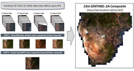
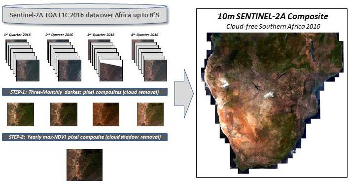
:The processing of cloud free geo-referenced imagery is one of the preliminary processing steps of any land application. This letter describes the methodology developed to obtain a seamless cloud free composite of Africa for 2016 using Sentinel-2A data at 10-meter resolution freely available from the European Space Agency. The method is based on a hybrid method resulting from the merging of the two most robust time series methods namely the “darkest pixel” and the “maximum Normalised Difference Vegetation Index (NDVI)” previously developed with the Advanced Very-High-Resolution Radiometer (AVHRR) time series.
1. Introduction
As part of the Copernicus programme of the European Union (EU), the European Space Agency (ESA) has developed and is operating the Sentinel-2 mission acquiring high spatial resolution optical imagery [1]. The space component of Copernicus programme consists of five missions: Sentinel 1–5 [2], designed to provide routine observations to establish a European capacity for environment and security applications and ensure data continuity to heritage missions (e.g., ERS, Envisat, SPOT and Landsat) improving observational capabilities [3,4].
The Sentinel-2 mission offers an unprecedented combination of systematic global coverage of land coastal areas between −56 and +84 degrees latitude, a high revisit under the same viewing conditions, high spatial resolution 10–60 m, and a wide field-of-view of 290 km for multispectral observations from 13 bands in the visible, near infrared and short wave infrared range of the electromagnetic spectrum [1,3]. The revisit time is 10 days at equator with only Sentinel-2A (S2A), but thanks to the successful launch of Sentinel-2B (S2B) on 7 March 2017, and the resulting availability of S2B data after the commissioning phase will decrease the revisit time to 5 days.
The potential of Sentinel-2 MSI includes a wide range of applications: agriculture, forestry, land use planning and infrastructure development.
As reported in the conclusion of the ESA WorldCover 2017 conference (http://worldcover2017.esa.int/), the main objective of land-cover users, is to have a global high resolution (HR) land cover map, and the first step to obtain this is to generate HR cloud-free composites using as input optical imagery time series.
In order to fully exploit this optical HR time series we should consider the effect of data gaps related to clouds and cloud shadow that represent a limiting factor. From 2008, when Landsat archive with data from 1970s was opened, several scientists attempted to produce HR cloud- and gap-free maps using various approaches based on temporal composited mosaicking, pixel based compositing and spatial-temporal gap-filling [5].
The main objective of this activity was to develop a method based on Sentinel-2A (S2A) data to produce a cloud-free composite over Southern Africa up to 8° S at 10-meter resolution. The S2A data have been acquired from 1 January 2016 to 5 December 2016, the end date does not coincide to the end of the year due to the change in the S2A data format, and the resulting impossibility in reading the data with SeNtinel Application Platform (SNAP) v4 [6] installed in our system. The input data have been processed using temporal-based method which extracts the complementary information from other data acquired at the same position and at different time periods [7], with an innovative ‘two-steps’ algorithm based on three-monthly darkest pixel selection to remove clouds and successively yearly composite based on maximum NDVI to further remove cloud shadows. The area of interest (AOI) covers a surface of about 7,430,000 km² and has been processed from 740 S2A L1C granules, also called “tiles”, (110 km × 110 km, at 10 m spatial resolution).
The time series of S2A images has been processed using a CalESA system, described in the next paragraph. The yearly composites are based on S2A L1C tiling grid (110 km × 110 km) and then mosaicked using GDAL utilities and Python routines based on the geo-location information associated to the pixels included in the metadata.
2. Materials and Methods
2.1. System Description
Due to the quantity of S2A L1C data over the AOI, more than 30,000 S2A L1C images have been used as input with a total size of 15 TB, a system for semi-automatic generation of cloud-free composite has been developed. This approach allows us to use the same resources for data storage and processing.
Processing of the S2A data was done on CalESA system, a cluster composed of 21 server PC, 2 Tower server PC, 1 GB network switch, that summarise 120 CPU Core, 580 GB shared Memory and 386 TB storage space. CalESA system comprises the cluster powered by Hadoop, the EO data processing system and the Distributed File System, that stores S2A data. The processing system comprises a processor adapter allowing to integrate Unix or python scripts and SNAP processor.
The system is based on Hadoop 2.7 and Calvalus [8] with SNAP-core. Logical system hierarchy is as follow: (1) Master PC for process management and HDFS supervision, 20 nodes (slaves) PC for processing and HDFS storage and (2) additional PC for downloading and products ingestion (and products translation for viewer).
Basic platform components (Table 1):
2.2. Algorithm Description
2.2.1. Pre-Processing
The S2A L1C products [9,10] provide Top Of Atmosphere (TOA) normalized reflectances for each spectral band in Universal Transverse Mercator (UTM) coordinate system (CS) based on WGS-84 ellipsoid, this system divides the Earth between 80°S and 84°N latitude into 60 zones, each 6° of longitude in width. The S2A L1C granules (a granule is the minimum indivisible partition of a product), are based on the Military Grid Reference System (MGRS) tiles with an overlap with neighbouring tiles. The 110 km × 110 km footprint of each tile can be obtained in a Keyhole Mark-up Language (KML) file [11]. The S2A L1C products distributed before 5 October 2016 on Sentinels DataHub are packaged in multi-L1C tile containing more than one S2A L1C granule (110 km × 110 km), used as basis for the cloud-free composite. This requires a preliminary action to extract each of L1C tile in order to create a stack of data based on S2A L1C tiling grid [11].
Due to the abundance of S2A data, in order to reduce the computation time, we decided to apply a preliminary screening based on cloud coverage information reported in the CLOUDY_PIXEL_PERCENTAGE field of the metadata (less than 5%), discarding approximately 37% of the total amount of S2A products archived on Copernicus Open Access Hub (available at https://scihub.copernicus.eu/). The cloud mask indicates the percentage of cloud coverage (cirrus and opaque), and it is computed for each Level-1C Granule using threshold algorithm based on Blue, B10 (1375 nm) and SWIR bands.
If the S2A L1C granule is not covered with at least three images with a cloud coverage less than 5% for each Quarter, it is marked as an “area with high persistency of clouds” and all the S2A L1C products in the catalogue will be taken as input in order to use all the available pixels. At the end of this preliminary analysis we selected more than 30,000 S2A L1C product as input of the processing chain.
The original S2A L1C products are in Universal Transverse Mercator (UTM) coordinate system (CS) based on WGS-84 ellipsoid, this system divides the Earth between 80°S and 84°N latitude into 60 zones, each 6° of longitude in width but it cannot be applied as CS to map the entire Africa. For this reason, we re-projected all S2A L1C products included in the AOI (up to 8°S) in Geographic Latitude and Longitude CS.
The achievement of the objective was possible because S2A L1C product geo-location is very good, better than 10 m RMS respecting the initial mission requirements. In fact, during the pre-processing, we did not apply any geometric correction on the input data [1].
2.2.2. Darkest Pixel Method
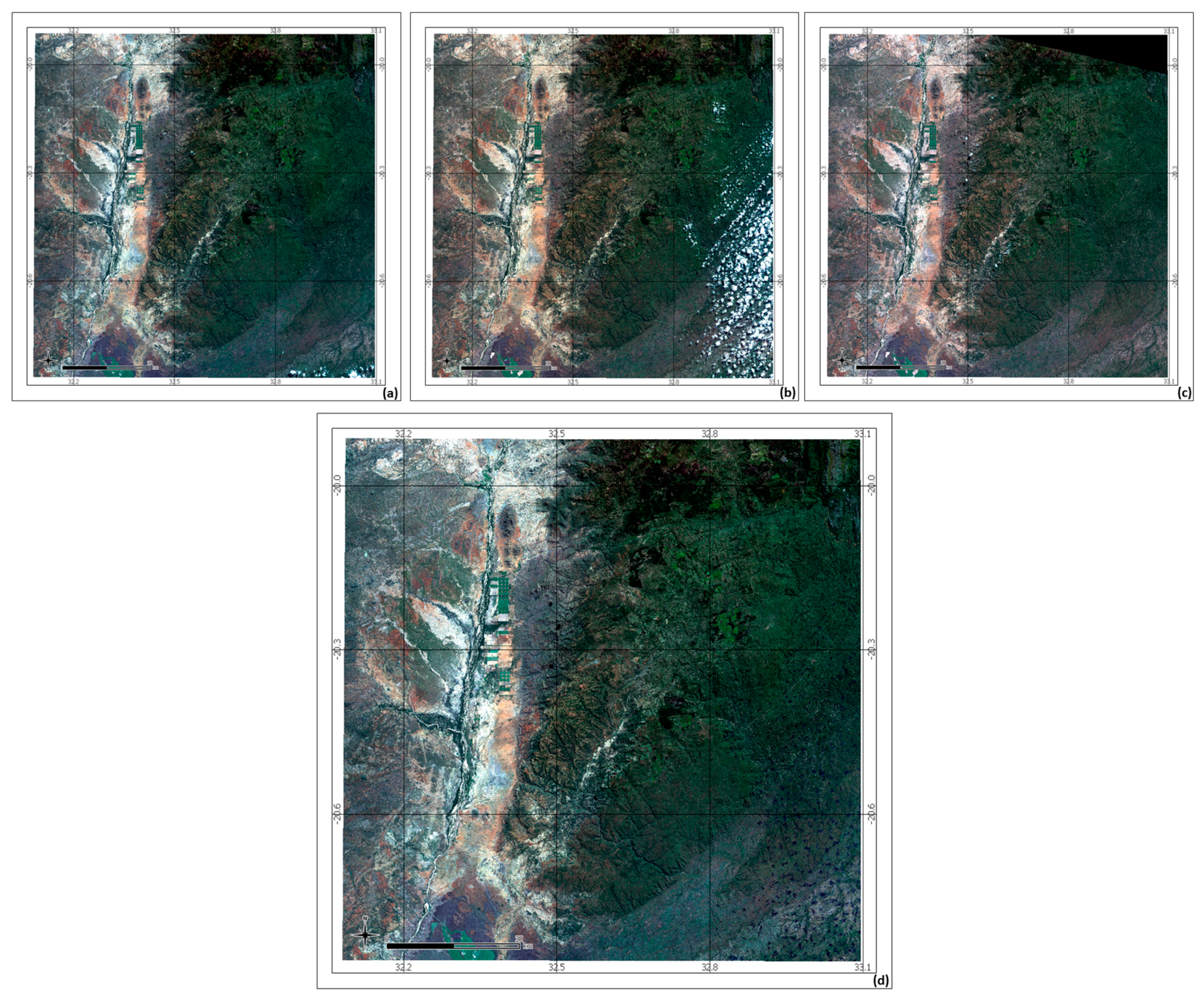
Usually, to generate cloud-free maps, complex algorithms for cloud detection and removal are applied, such as Sen2Cor (Scene Classification and cloud mask) [12], Automated Cloud-Cover Assessment Algorithm (ACCA) [13] or F-mask [14]. Using the mentioned algorithms, it is possible to improve the quality of the output, but the weak points are the difficulties to customise the parameters and the increasing of the computation time (e.g., to run Sen2Cor on a single S2A L1C granule at 10 m resolution one hour is needed). Therefore, to reduce computation time maintaining a good quality of the output, we decided to use a simpler method that allows us to replace cloudy pixels with cloudless ones (if present in the stack of S2A images) choosing the darkest value for each of the 10-meter bands (visible and Near Infra-Red). The reference period for the darkest pixel selection is three months in order to have a sufficient number of S2A L1C data (3 images per month with the current coverage) and to respect the seasonality (Figure 2).
As described by Saunders [15], in the histogram of visible reflectance, the land and water peaks are well defined at the ‘dark’ end with cloudy reflectance producing a broad higher reflectance tail.
The darkest pixel method generates as its intermediate output three-monthly composites replacing cloudy pixels with cloudless ones (if present in the S2A L1C data stack) marking as valid also pixels affected by cloud shadows that will be removed in the second step of the algorithm, described below.
2.2.3. Maximum NDVI Method
The Normalised Difference Vegetation Index (NDVI) measures the spectral response of the vegetation and it is defined as the difference between near-infrared and red reflectance divided by the sum of the two (NIR − Red)/(NIR + Red). As reported by in the Maximum-Value Composite (MVC) procedure [16] and Best Index Slop Extraction (BISE) [17], any attenuation of the spectral signals will reduce the NDVI value from that of an unattenuated signal. Therefore, the best possible pixel value for a particular location is achieved by choosing the highest NDVI pixel value from multi-temporal data (Figure 3). The maximum NDVI method shows seasonal effect due to the selection of greenest value from quarterly intermediate outputs influencing the homogeneity of the map when the S2A L1C yearly granules over the AOI are mosaicked, but it does not affect our main objective to create a cloud-free map.
2.2.4. Combining Method
Comparing the output of the two methods described above, we observed that each method taken individually is insufficient, and for this reason we combined them in the most efficient manner considering the computation time and final results.
STEP-1—To remove the clouds, for each quarter (January–March, April–June, July–September, October–December) darkest pixel selection from the stack of S2A L1C TOA images identified as input.
STEP-2—From the quarterly composites choose the best pixel applying the “max-NDVI” method replacing the pixels affected by cloud shadow with clear ones, if present.
The overall computation time to generate a yearly cloud-free composite for a single S2A L1C granule is around 2 h, lower than the classical methods using cloud mask and atmospheric correction. In fact, if we would apply Sen2Cor for cloud detection and atmospheric correction we will increase the time by one hour for each S2A L1C image in input, in the best case (only 3 inputs for each quarterly) the processing time would reach around 14 h to generate yearly cloud-free composite per single S2A L1C granule increasing the time by a factor of 7 that becomes 19 in the worst case (9 inputs for each quarterly).
2.2.5. Post-Processing
To visualise the final product, we developed a series of python scripts that combine different GDAL utilities described by R. Simmons [18], applying histogram stretching to the RGB bands, data compression and generating an overview at different zoom levels of each S2A L1C TOA tile.
The non-homogeneity of the final product is due to our processing method being based on a single S2A L1C granule. In fact, each of S2A L1C tile is processed independently using S2A data over the AOI respecting the criteria and methods described in the previous paragraphs and if the inputs are acquired in different seasons the radiometry, especially in vegetated areas, changes consistently. A good atmospheric correction could minimize this issue, but, as already highlighted, it will increase enormously the computation time.
To display and interact with the map on the web page we used Leaflet an open-source JavaScript library.
3. Results
The cloud-free map over Africa up to 8°S using S2A L1C data from 1 January to 5 December 2016, shown in Figure 4 is available at http://2016africacomposite10m.esrin.esa.int/. Comparing visually our result to the Global Web-Enabled Landsat Data (WELD) [18] for the year 2011 (available at https://globalweld.cr.usgs.gov/distribution_global.php) at 30 m generated from Landsat 7 ETM+ and Landsat 5 TM data, is possible to observe that the quality of our product in terms of cloud and cloud shadow removal over the AOI is very similar to Global-WELD even if both of them show artefacts over tropic region due to the cloud persistency and over water surface.
Two weak points of our product are represented by: (a) water surface where, in some cases, our method is not strong enough to discard clouds due to low value of NDVI; (b) non-homogeneity of the map already is explained in Section 2.2.3.
4. Discussion
In recent years, with the abundance of HR optical data being freely available (Sentinel-2 and Landsat), the increasing cloud computation power and the related cost reduction, the interest of scientists and commercial companies is increasingly focussing on HR cloud-free composite applying several approaches spatial-/temporal-/spectral-based.
The main objective of this study is to develop a computational efficient method to produce a cloud-free map over a continental scale implementing a suit of simple algorithms for cloud and cloud shadow removal using a temporal-based approach, considering as a key requirement that the output has to be generated quickly.
In order to be compliant with this constraint, we decided to not apply atmospheric correction. In fact, as already explained in Section 2.2.4, applying Sen2Cor the computation time will increase by a factor from 7 to 19, depending from the number of S2A L1C TOA images taken as input in the darkest pixel selection.
The ‘two steps’ algorithm is based on two methods developed and applied in the past for AVHRR data [15,16,17], which are different in terms of space resolution, revisit time and spectral bands from Sentinel-2. Despite the differences between the two sensors listed above, we decided to test and combine, successfully, ‘darkest pixel’ and ‘maximum NDVI‘ pixel selection in order to replace cloudy and cloud shadow pixels respectively.
By visual inspection (http://2016africacomposite10m.esrin.esa.int/) any user can see that the obtained result is fully achieved.
The near-future activities of this methodological development will be focused to the whole of Africa, particularly within the tropical forest biome. Then, they will be applied to another continent to further evaluate the robustness and efficiency of the developed method.
5. Conclusions
A new temporal-based composite method has been developed and tested for Sentinel-2 TOA L1C time series. After a visual inspection, results are very encouraging especially due to the cloud coverage over the AOI, although we observed problems in clouds removal from water surface and non-homogeneity of the final product.
The strong points of this method are the easy implementation, the quick computation time and the possibility to export and to adapt it easily to cloud processing systems expanding the AOI and the period.
Acknowledgments
The S2A Level 1C TOA data have been kindly provided by Eric Monjoux and Adriana Grazia Castriotta from ESA Payload Data Ground Segment (PDGS). The comments and suggestions from the two referees have been very constructive.
Conflicts of Interest
The authors declare no conflict of interest.
References
- Gascon, F.; Thépaut, O.; Jung, M.; Francesconi, B.; Louis, J.; Lonjou, V.; Lafrance, B.; Massera, S.; Gaudel-Vacaresse, A.; Languille, F.; et al. Copernicus Sentinel-2 Calibration and Products Validation Status. Remote Sens. 2017, 9, 584. [Google Scholar] [CrossRef]
- Berger, M.; Moreno, J.; Johannessen, J.A.; Levelt, P.F.; Hanssen, R.F. ESA’s sentinel missions in support of Earth system science. Remote Sens. Environ. 2012, 120, 84–90. [Google Scholar] [CrossRef]
- Drusch, M.; Del Bello, U.; Carlier, S.; Colin, O.; Fernandez, V.; Gascon, F.; Hoersch, B.; Isola, C.; Laberinti, P.; Martimort, P.; et al. Sentinel-2: ESA’s optical high-resolution mission for GMES operational services. Remote Sens. Environ. 2012, 120, 25–36. [Google Scholar] [CrossRef]
- Aschbacher, J.; Milagro-Pérez, M.P. The European Earth monitoring (GMES) programme: Status and perspectives. Remote Sens. Environ. 2012, 120, 3–8. [Google Scholar] [CrossRef]
- Vuolo, F.; Ng, W.-T.; Atzberger, C. Smoothing and gap-filling of high resolution multi-spectral time series: Example of Landsat data. Int. J. Appl. Earth Obs. Geoinf. 2017, 57, 202–213. [Google Scholar] [CrossRef]
- European Space Agency. Sentinel Application Platform (SNAP). 2017. Available online: http://step.esa.int/main/toolboxes/snap/ (accessed on 15 June 2017).
- Shen, H.; Li, X.; Cheng, Q.; Zeng, C.; Yang, G.; Li, H.; Zhang, L. Missing information reconstruction of remote sensing data: A technical review. IEEE Geosci. Remote Sens. Mag. 2015, 3, 61–85. [Google Scholar] [CrossRef]
- Fomferra, N.; Böttcher, M.; Zühlke, M.; Brockmann, C.; Kwiatkowska, E. Calvalus: Full-mission EO cal/val, processing and exploitation services. In Proceedings of the 2012 IEEE International Geoscience and Remote Sensing Symposium (IGARSS), Munich, Germany, 22–27 July 2012. [Google Scholar]
- European Space Agency. Sentinel-2 Products Specification Document. 2017. Available online: https://sentinel.esa.int/documents/247904/349490/S2_MSI_Product_Specification.pdf (accessed on 15 June 2017).
- Sentinel-2 L1C Tiling Grid. 2017. Available online: https://sentinel.esa.int/web/sentinel/missions/sentinel-2/data-products (accessed on 15 June 2017).
- European Space Agency. Level-2A Prototype Processor for Atmosphericterrain and Cirrus Correction of Top-of-Atmosphere Level 1C Input Data. 2017. Available online: http://step.esa.int/main/third-party-plugins-2/sen2cor/ (accessed on 15 June 2017).
- Irish, R.R.; Barker, J.L.; Goward, S.N.; Arvidson, T. Characterization of the Landsat-7 ETM+ Automated Cloud-Cover Assessment (ACCA). Photogramm. Eng. Remote Sens. 2006, 72, 1179–1188. [Google Scholar] [CrossRef]
- Zhu, Z.; Wang, S.; Woodcock, C.E. Improvement and expansion of the Fmask algorithm: cloud, cloud shadow, and snow detection for Landsats 4–7, 8, and Sentinel 2 images. Remote Sens. Environ. 2015, 159, 269–277. [Google Scholar] [CrossRef]
- Saunders, R.W.; Kriebel, K.T. An improved method for detecting clear sky and cloudy radiances from AVHRR data. Int. J. Remote Sens. 1998, 9, 123–150. [Google Scholar] [CrossRef]
- Holben, B.N. Characteristics of Maximum Value Composite images from temporal AVHRR data. Int. J. Remote Sens. 1986, 7, 1417–1434. [Google Scholar] [CrossRef]
- Viovy, N.; Arino, O.; Belward, A.S. The Best Index Slope Extraction (BISE): A method for reducing noise in NDVI time-series. Int. J. Remote Sens. 1992, 13, 1585–1590. [Google Scholar] [CrossRef]
- Simmons, R. A Gentle Introduction to GDAL Part 4: Working with Satellite Data. 2017. Available online: https://medium.com/@robsimmon/a-gentle-introduction-to-gdal-part-4-working-with-satellite-data-d3835b5e2971 (accessed on 15 June 2017).
- Roy, D.P.; Ju, J.; Kline, K.; Scaramuzza, P.L.; Kovalskyy, V.; Hansen, M.; Loveland, T.R.; Vermote, E.; Zhang, C. Web-enabled Landsat Data (WELD): Landsat ETM+ composited mosaics of the conterminous United States. Remote Sens. Environ. 2010, 114, 35–49. [Google Scholar] [CrossRef]
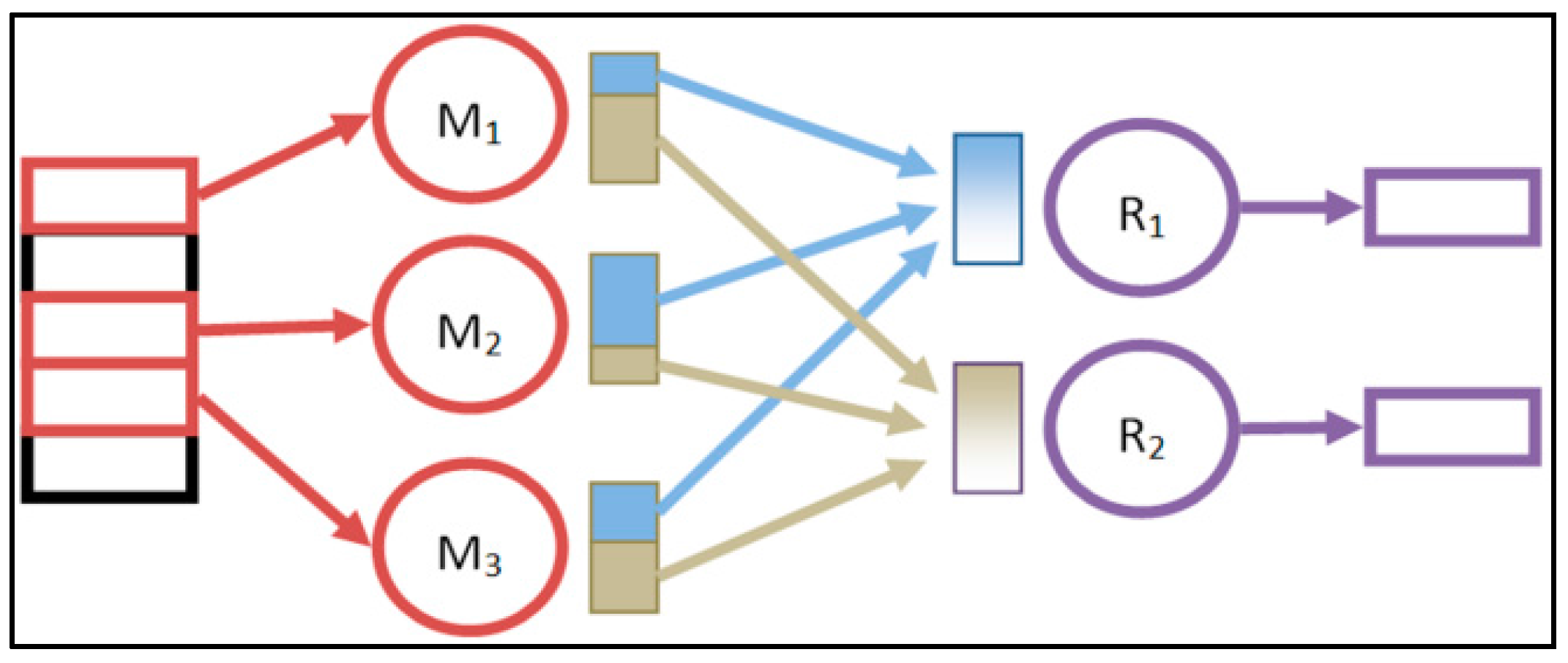
Figure 1.
Hadoop computational paradigm—Map, Reduce and Formatting functions.

Figure 2.
The figure shows the output of the darkest pixel method, it selects the lowest Top Of Atmosphere (TOA) reflectance value for each of the 10-meter bands (visible and Near Infra-Red) taking into account three months of data. (a) S2A image acquired on 04/05/2016; (b) S2A image acquired on 14/05/2016; (c) S2A image acquired on 24/05/2016; (d) 2nd Quarter 2016 composite based on darkest pixel selection, black spots are cloud shadows as consequence of darkest pixel selection. © Contains modified Copernicus Sentinel data (2016)/Processed by the European Space Agency (ESA).

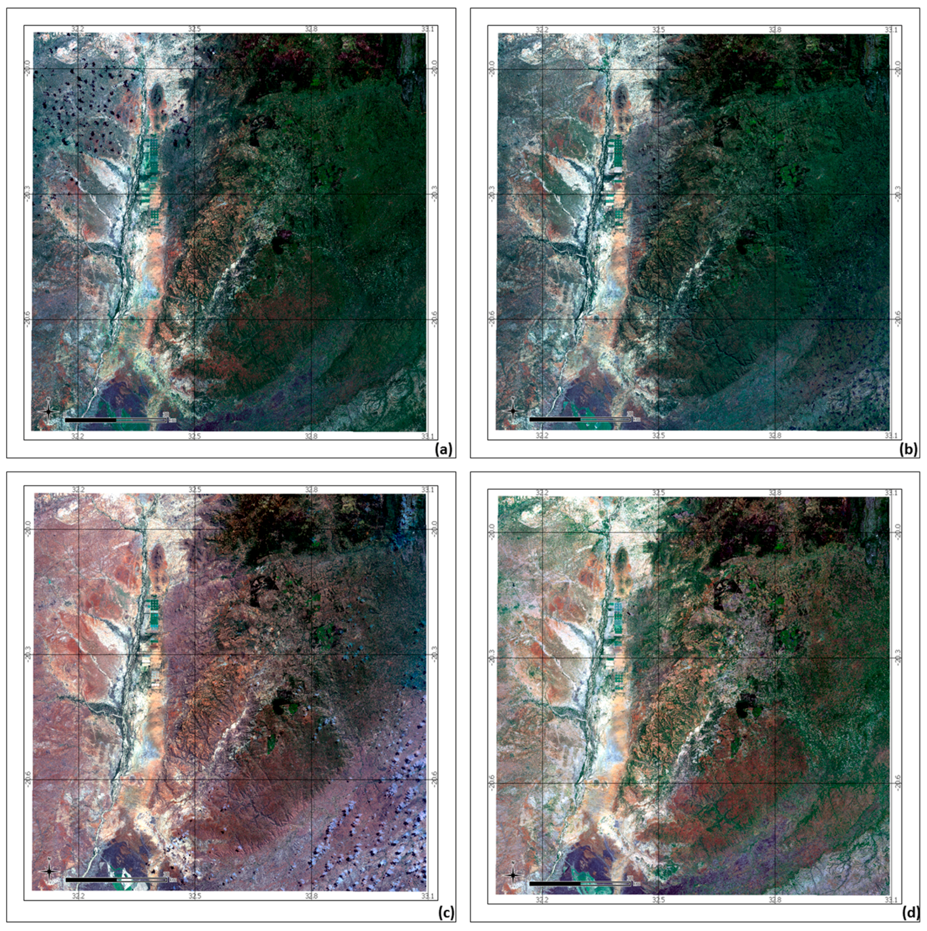
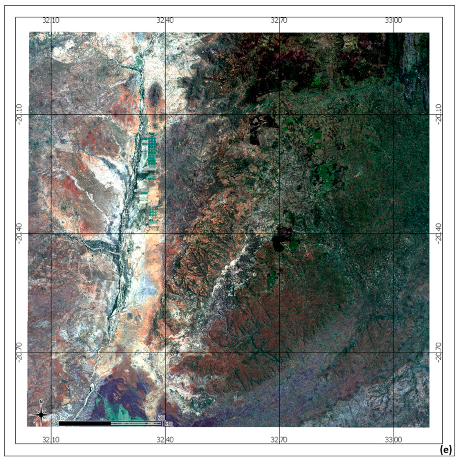
Figure 3.
The figure shows the output of the Max-Normalised Difference Vegetation Index (NDVI) method, it selects the greenest value from quarterly intermediate products removing cloud shadows. (a) Darkest pixel composite for 1st Quarter 2016; (b) Darkest pixel composite for 2nd Quarter 2016; (c) Darkest pixel composite for 3rd Quarter 2016, on bottom right of the image is possible to observe how the clouds have been replaced by clear pixels even if the reflectance is higher respect to neighbour pixels; (d) Darkest pixel composite for 4th Quarter 2016; (e) Yearly composite based on Max-NDVI. © Contains modified Copernicus Sentinel data (2016)/Processed by ESA.


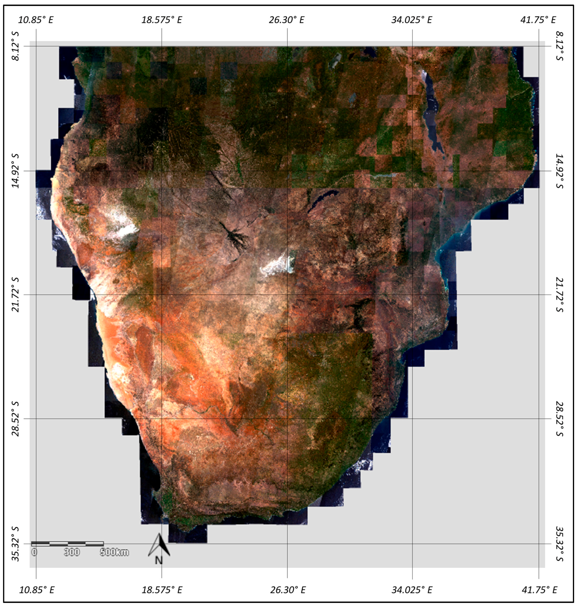
Figure 4.
S2A cloud-free yearly composite—Southern Africa up to 8°S. S2A L1C granules over the AOI have been mosaicked using natural color RGB composition at 10m spatial resolution. © Contains modified Copernicus Sentinel data (2016)/Processed by ESA.
Figure 4.
S2A cloud-free yearly composite—Southern Africa up to 8°S. S2A L1C granules over the AOI have been mosaicked using natural color RGB composition at 10m spatial resolution. © Contains modified Copernicus Sentinel data (2016)/Processed by ESA.


Table 1.
Basic platform components.
| Operating System | Hadoop | Java | Calvalus |
|---|---|---|---|
| CentOS 6.8 | 2.7.2 | Oracle java 8 | 2.9 with SNAP 4.0 |
Table 2.
Map Function description.
| Map Function (M1, …, Mn) |
|---|
| Reads inputs (all available bands) Re-projects the source pixels to the target grid (same resolution) Sorts the result pixels into different partitions of the target grid, one per reducer Forwards the partitions to the reducers |
Table 3.
Reduce Function description.
| Reduce Function (R1, …, Rj) |
|---|
| Sorts the contributions by target grid pixel and time Applies the temporal aggregator (to all selected bands) Writes one part of the global result pixel by pixel (all selected bands) |
Table 4.
Formatting Function description.
| Formatting Function |
|---|
| Concatenates the intermediate products and exports the final output in Network Common Data Form (NetCDF) format. |
© 2017 by the authors. Licensee MDPI, Basel, Switzerland. This article is an open access article distributed under the terms and conditions of the Creative Commons Attribution (CC BY) license (http://creativecommons.org/licenses/by/4.0/).
Share and Cite
MDPI and ACS Style
Ramoino, F.; Tutunaru, F.; Pera, F.; Arino, O. Ten-Meter Sentinel-2A Cloud-Free Composite—Southern Africa 2016. Remote Sens. 2017, 9, 652. https://doi.org/10.3390/rs9070652
AMA Style
Ramoino F, Tutunaru F, Pera F, Arino O. Ten-Meter Sentinel-2A Cloud-Free Composite—Southern Africa 2016. Remote Sensing. 2017; 9(7):652. https://doi.org/10.3390/rs9070652
Chicago/Turabian StyleRamoino, Fabrizio, Florin Tutunaru, Fabrizio Pera, and Olivier Arino. 2017. "Ten-Meter Sentinel-2A Cloud-Free Composite—Southern Africa 2016" Remote Sensing 9, no. 7: 652. https://doi.org/10.3390/rs9070652
Note that from the first issue of 2016, this journal uses article numbers instead of page numbers. See further details here.