Article

A Satellite-Derived Climatological Analysis of Urban Heat Island over Shanghai during 2000–2013

1
Department of Land Management, Zhejiang University, Hangzhou 310058, China
2
Key Laboratory of Agricultural Remote Sensing and Information Systems, Hangzhou 310058, China
3
Key Laboratory of Environment Remediation and Ecological Health, Ministry of Education, Zhejiang University, Hangzhou 310058, China
4
Shanghai Climate Center, Shanghai Meteorological Bureau, Shanghai 200030, China
5
Institute of Applied Remote Sensing and Information Technology, College of Environmental and Resource Sciences, Zhejiang University, Hangzhou 310058, China
6
Department of Agro-Meteorology and Geo-Informatics, Magbosi Land, Water and Environment Research Center (MLWERC), Sierra Leone Agricultural Research Institute (SLARI), Tower Hill, Freetown PMB 1313, Sierra Leone
*
Author to whom correspondence should be addressed.
Remote Sens. 2017, 9(7), 641; https://doi.org/10.3390/rs9070641
Submission received: 17 April 2017 / Revised: 6 June 2017 / Accepted: 19 June 2017 / Published: 22 June 2017

Abstract

:
The urban heat island is generally conducted based on ground observations of air temperature and remotely sensing of land surface temperature (LST). Satellite remotely sensed LST has the advantages of global coverage and consistent periodicity, which overcomes the weakness of ground observations related to sparse distributions and costs. For human related studies and urban climatology, canopy layer urban heat island (CUHI) based on air temperatures is extremely important. This study has employed remote sensing methodology to produce monthly CUHI climatology maps during the period 2000–2013, revealing the spatiotemporal characteristics of daytime and nighttime CUHI during this period of rapid urbanization in Shanghai. Using stepwise linear regression, daytime and nighttime air temperatures at the four overpass times of Terra/Aqua were estimated based on time series of Terra/Aqua-MODIS LST and other auxiliary variables including enhanced vegetation index, normalized difference water index, solar zenith angle and distance to coast. The validation results indicate that the models produced an accuracy of 1.6–2.6 °C RMSE for the four overpass times of Terra/Aqua. The models based on Terra LST showed higher accuracy than those based on Aqua LST, and nighttime air temperature estimation had higher accuracy than daytime. The seasonal analysis shows daytime CUHI is strongest in summer and weakest in winter, while nighttime CUHI is weakest in summer and strongest in autumn. The annual mean daytime CUHI during 2000–2013 is 1.0 and 2.2 °C for Terra and Aqua overpass, respectively. The annual mean nighttime CUHI is about 1.0 °C for both Terra and Aqua overpass. The resultant CUHI climatology maps provide a spatiotemporal quantification of CUHI with emphasis on temperature gradients. This study has provided information of relevance to urban planners and environmental managers for assessing and monitoring urban thermal environments which are constantly being altered by natural and anthropogenic influences.

Graphical Abstract

1. Introduction

Urbanization has accelerated in the recent past and is likely to accelerate further in the coming decades. Conversely, natural spaces are decreasing in many areas in response to urbanization. Currently, approximately 54% of the world’s population lives in urban areas, and this proportion is expected to increase to 66% by 2050 [1]. The rapid urbanization process leads to the replacement of natural surfaces with man-made features such as pavements, buildings and other infrastructure, which have altered the radiative, thermal, and moisture properties of the urban environment [2,3]. In addition, population growth in urban areas has increased anthropogenic heat generated from traffic use, air conditioning facilities, and industrial activities. As a result, urban areas tend to have higher air or surface temperatures than surrounding rural areas, a phenomenon known as the urban heat island (UHI). UHI has caused significant impacts on environmental quality and human well-being in urban areas, prominent among which include the increase in energy consumption for cooling [4,5], elevation in air pollutant concentrations [6], exacerbating heat waves which cause serious human discomfort and related health and mortality problems [7,8,9], inducing local or regional climate variability and change [10,11], and the increase in urban carbon footprints [12]. These adverse effects are even more pronounced in metropolitan areas, especially where there is an ever increasing population density and extensive anthropogenic activities. Therefore, studying the spatiotemporal characteristics of UHI has been of great importance to improve our understanding of the intra-urban and inter-urban temperature distribution, the vulnerability to heat risk of urban human populations, and human-environmental interactions [13,14].
UHI phenomenon describes the excess warmth of the urban atmosphere and surfaces compared to the non-urbanized rural surroundings. Heat islands can be characterized at different layers of the urban atmosphere and for various surfaces and can be divided into three categories: canopy layer urban heat island (CUHI), boundary layer urban heat island (BLHI), and surface urban heat island (SUHI). The urban canopy layer (UCL) refers to the layer of the urban atmosphere between the ground level and approximately mean building height, whereas the urban boundary layer is located above the canopy layer [10]. CUHI and BLHI are atmospheric heat islands since they denote a warming of the urban atmosphere, whereas the SUHI refers to the relative warmth of urban surfaces compared to surrounding rural areas. CUHI is normally measured by air temperatures from weather station networks or from traverses of vehicle-mounted sensors. BLHI observations are made from more specialized sensor platforms such as tall towers, radiosonde or tethered balloon flight. SUHI is typically measured as land surface temperature (LST) through airborne or satellite thermal infrared remote sensing. UHI intensity is a widely used indicator to quantify UHI, which is defined as the air or land surface temperatures between urban and rural areas. SUHI research is thriving after LST data become available [15,16,17,18,19,20,21,22]. Most previous SUHI studies [23,24,25,26,27] focus on its temporal evolution, spatial patterns, and its relationship with land surface properties such as land cover types, percent impervious area, and normalized difference vegetation index (NDVI).
CUHI is more closely related to mortality during extreme heat events than SUHI. The CUHI has been extensively studied for many major cities in the world like Tokyo [28], New York [29], Seoul [30], Hong Kong [31], Singapore [32], and Beijing [33,34]. In addition, the CUHI has also been investigated in small and medium-scale cities such as Lodz [35], Volos [36], and Granada [37]. Since the 1980s, there have been a number of studies investigating CUHI in Shanghai. Zhou et al. [38] investigated the annual, seasonal, and fixed hourly variations of the Shanghai CUHI in urban and suburban areas. Deng et al. [39] analyzed the characteristics of CUHI based on air temperatures measured by Davis automatic stations installed in the urban and suburb areas of Shanghai at 1998–1999. The CUHI intensity is quantified by calculating air temperature differences between urban and suburb stations. The mean value of air temperature at Xuhui, Changing, and Pudong stations was taken as urban temperature. The temperature of the northwestern station was taken as suburb temperature. The result showed that the monthly mean CUHI intensity was greater than 0.8 °C and the seasonal mean CUHI intensity was stronger in autumn and winter than in summer. Zhao et al. [40] found out that the difference in mean annual temperature between urban and rural stations increased from 0.1 °C in the late 1970s to 0.7 °C in the early 2000s, with an increase of 0.24 °C per decade. Moreover, Zhang et al. [41] investigated the temporal variations and spatial distribution of Shanghai CUHI and found out that CUHI was strongest in autumn and weakest in summer, temporal patterns which are closely tied to the prevailing weather conditions. More recently, Zhang et al. [42] reported an average CUHI intensity of 1.17 °C for 86% of the days of the year, and that the frequency and intensity of CUHI in autumn were higher than those in other seasons. They also stated that the accumulated intensities of daytime CUHI at 14:00 are significant in spring and summer, and those at 08:00 are more evident in autumn and winter.
In most previous studies, air temperature for quantifying CUHI is traditionally collected from stationary meteorological stations, which provide point data with a high temporal frequency. However, the spatial information of air temperature is often very limited due to the sparse distribution of meteorological stations [43]. Moreover, the limited footprints of ground-based measurements make it difficult to capture a comprehensive distribution of air temperature over highly heterogeneous urban areas [44]. This is particularly important in thermally complex urban environments where local microclimatic variability is influenced by factors such as land cover, exposure to wind and sun, soil and vegetation moisture, and the thermal properties of upwind areas [45,46]. To solve these problems, usually a well-designed network of stations is required. Perhaps, a consistent gridded dataset of observations from satellite remote sensing may be an easy and straightforward approach for the acquisition of spatially continuous air temperature data.
Unlike in situ measurements, space-borne remote sensing provides an additional source of data with high resolution and spatially explicit information, which enables the monitoring of UHIs at large scales and enables detection of urban areas in which the heating effect is more pronounced [14]. Remotely sensed images with relatively high spatial resolution, such as the Landsat Thematic Mapper (TM), Enhanced Thematic Mapper Plus (ETM+), Operational Land Imager (OLI) and the Terra Advanced Space-borne Thermal Emission and Reflection Radiometer (ASTER) data, are widely used to study urban thermal patterns and their relationships with surface characteristics in SUHI studies [25,47,48,49,50]. However, it is difficult to characterize and examine UHIs consistently or to monitor UHIs in near-real time due to the limited temporal coverage of Landsat TM/ETM+/OLI and ASTER data. On the other hand, remotely sensed data with higher temporal resolutions, such as the Moderate Resolution Imaging Spectroradiometer (MODIS) on board Aqua and Terra, provide the possibility to monitor UHI variations at different temporal scales, though at a spatial resolution of 1 km. The temporally consistent LST at global scales derived from satellite remotely sensed data provides a way to estimate spatially continuous air temperatures for CUHI studies.
In recent years, many studies have been conducted on the estimation of air temperature from remotely sensed data. Due to the complexities of atmospheric radiance and its low proportion in remotely sensed signals, it is difficult to directly derive near-surface air temperature from satellite thermal data [51]. The air temperature is mostly estimated based on remotely sensed land surface temperature. The temperature–vegetation index (TVX) method [52,53,54] and the statistical methods [43,51,55,56,57,58] are two commonly used methods for estimating air temperature. To link LST and air temperature, many factors must be considered, such as the surface properties, atmospheric conditions and solar angles [59,60]. MODIS data can provide spatial information on many of the factors that influence air temperature and can be useful in mapping in spatially heterogeneous environments. Thus, air temperature estimated from satellite remote sensing data has a great potential for application in human health related research, and long term temperature data records of more than 10 years can provide a platform for producing CUHI climatology maps in space and time.
Despite several awareness and research on CUHI in the world, few studies have been conducted on climatological analysis of CUHI during the rapid urbanization using time series remotely sensed data. Previous studies in Shanghai have mainly concentrated on SUHI [22,23,25,27], whereas in this paper the emphasis is put on CUHI. The most prominent CUHI studies conducted in Shanghai in the recent past [41,42,61] employed meteorological data obtained from conventional ground weather stations, which are disadvantaged by their inability to adequately describe or account for spatial heterogeneity over small geographic extents. Therefore, the present study aims at assessing the seasonal and spatial variability of CUHI and produce monthly gridded CUHI climatology maps during the period 2000–2013 based on thermal remotely sensed data and meteorological observation data, taking the Shanghai metropolitan area as case study. In this study, we have integrated time series Terra/Aqua MODIS LST products with ground meteorological observations to map the CUHI climatology of Shanghai. Air temperature at the four overpass times of Terra/Aqua was estimated based on time series of MODIS LST and other auxiliary variables including enhancing vegetation index (EVI), normalized difference water index (NDWI), solar zenith angle (SZA), and distance to coast (DTC) using stepwise linear regression method. Temporal and spatial variability of daytime and nighttime CUHI and spatiotemporal relationships between CUHI and NDVI have been investigated in the current study.

2. Materials and Methods

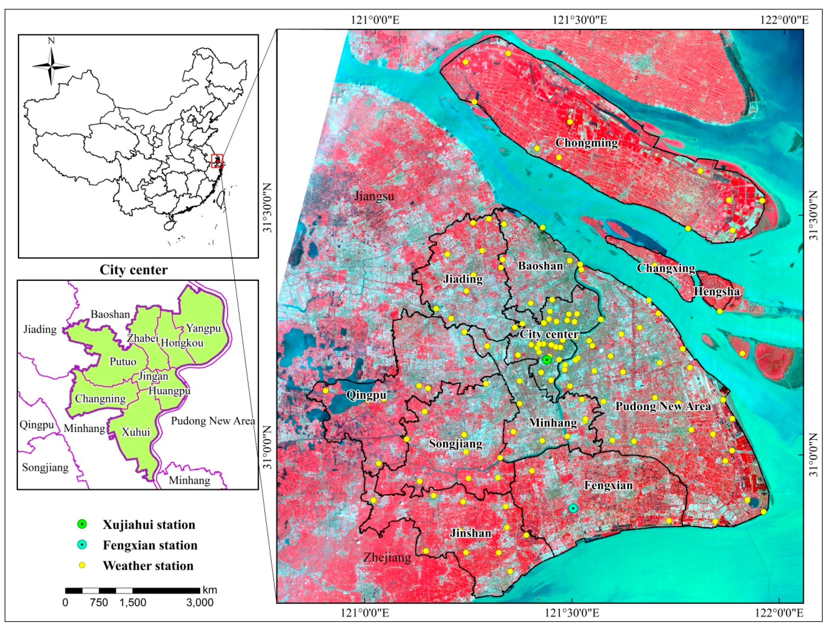
2.1. Study Area and Meteorological Station Data

The study area covers the Shanghai metropolis, which is located between latitudes 30°23′N to 31°27′N, and longitudes 120°52′E and 121°45′E (Figure 1). This area is characterized by a subtropical monsoon climate with a mean annual temperature of 17.2 °C, and monthly maximum and minimum mean temperatures of 30.2 °C in July and 1.9 °C in January, respectively. The mean annual precipitation is 1158.1 mm, with more than 60% of the rainfall occurring from May to September. The average elevation of Shanghai is about 4 m above sea level as it is largely located on a flat alluvial plain with a few remnant hills in the southwestern part of the metropolis.
Shanghai has historically been one of the most important economic centers in China since the early 1900s. This city has experienced a remarkable increase in urban area over the past 50 years with an unprecedented economic development initialized by the strategy of “opening of Pudong new area to the world” in the 1990s. Administratively, the Shanghai metropolis covers a total terrestrial area of 6450 km2. At present, Shanghai consists of 17 districts, namely, Huangpu, Xuhui, Changning, Jing’an, Putuo, Hongkou, Zhabei, Yangpu, Pudong New Area, Minhang, Baoshan, Jiading, Jinshan, Songjiang, Qingpu, Fengxian, and Chongming. According to the Shanghai Statistical Yearbook 2014, the city has a total population of about 24.15 million.
In this study, hourly air temperature during the period 2006–2013 was observed from 131 weather stations including 11 ordinary meteorological stations and a network of 120 automatic weather stations, and the data were obtained from the Meteorological Information Center of Shanghai Meteorological Bureau. These observations were taken in line with World Meteorological Organization (WMO) standards at 1.5 m above the ground. At non-urban stations recommended screen height is between 1.25 and 2 m above ground level. While this is also acceptable for urban sites, it may be better to relax this requirement to allow greater heights [62]. Furthermore, all the stations are located at relatively low elevations (<50 m) and in various environmental conditions. The 11 meteorological stations are the conventional observation stations distributed in 11 different districts, nanmely, Xujiahui, Pudong, Nanhui, Minhang, Baoshan, Jiading, Jinshan, Songjiang, Qingpu, Fengxian, and Chongming. The automatic weather stations have been made available in recent years, installed in accord with the operational standards issued by the China Meteorological Administration (CMA) and WMO. Being relatively distributed across Shanghai, they are designated to observe as many climatic variables as possible, including air temperature, wind, humidity, precipitation and so on. The availability of automatic weather stations has provided more spatial information for Shanghai. Figure 1 also shows the spatial distribution of weather stations in the Shanghai metropolis. Obviously, a large proportion of stations are located in the urban core, providing detailed weather information of inner city areas. However, not all the automatic weather stations were operational during the study period.
Since the temporal resolution of the data provided by weather stations is 1 h (recording at the top of every hour), linear interpolation was applied to obtain in situ air temperature at satellite overpass times (for Aqua, the overpass times are around 01:30 and 13:30 local solar time, whereas for Terra, the overpass times are around 10:30 and 22:30). The air temperature data covering the period 2006–2011 were used for model calibration, and the remaining air temperature observations (2012–2013) were used to validate the results of air temperature estimation.

2.2. MODIS Data and Pre-Processing

MODIS sensors were launched on board the National Aerodynamics and Space Administration (NASA) Earth Observing System (EOS) Terra and Aqua satellites in December 1999 and May 2002, respectively. The Terra overpass time is around 10:30 (local solar time) in its descending mode and 22:30 in its ascending mode. The Aqua overpass time is around 13:30 in its ascending mode and 01:30 in its descending mode.
Five MODIS products (v005) were used in this study: (1) Terra daily LST product (MOD11A1) from 2000 to 2013; (2) Aqua daily LST product (MYD11A1) from 2002 to 2013; (3) Land Cover Type product (MCD12Q1) from 2001 to 2012; and (4) Terra MODIS surface reflectance product (MOD09GA) from 2000 to 2013; (5) The monthly MODIS vegetation index products (MOD13A3). The 2012 land cover information was used for 2013 due to the unavailability of 2013 land cover data. These datasets are freely available from the NASA Reverb website (http://reverb.echo.nasa.gov/reverb). All the MODIS data were preprocessed using the MODIS Reprojection Tool (MRT). The data were first reprojected from the original Sinusoidal to the Universal Transverse Mercator (UTM) coordinate system (Zone 51N) with the WGS-84 datum as reference. In order to match the same spatial resolution with LST data, all the MODIS images were resampled into 1 km using the Nearest Neighbor resampling method. The MODIS land surface reflectance and LST data were then screened for cloud contamination with the state flags in MOD09GA, MOD11A1, and MYD11A1 products, respectively.

2.2.1. MODIS Land Surface Temperatures

Daily LST products (MOD11A1 and MYD11A1) with 1 km spatial resolution were produced with a generalized split window algorithm using the MODIS bands 31 and 32, which corrects for atmospheric effects and surface emissivity [63,64]. The accuracy of daily MODIS LST product was found to fall within 1 K under most clear-sky conditions. The overpass times of Terra occur at the approximate local solar times of 10:30 and 22:30; the overpass times of Aqua occur at the approximate local solar times of 01:30 and 13:30. Thus, within a day, MODIS can provide four LST observations. The four LST observations—Terra Day (TD), Terra Night (TN), Aqua day (AD), and Aqua night (AN)—are all used in this study.
The product are delivered in gridded HDF files for each tile which contain a number of scientific data sets (LST, quality control, view time and angle, emissivity of band 31 and 32, clear-sky coverage) which are array attributes of LST pixel values in each tile. Here, four day and night LST and quality control layers (LST_Day_1km, QC_Day, LST_Night_1km, QC_Night) were extract from the Terra/MOD11A1 and Aqua/MYD11A1 products, respectively. These data are gridded in the sinusoidal projection and have an accurate grid size of 0.926 km. We reprojected the data into UTM zone 51N, WGS84. The data were resampled from 0.926 to 1 km grid size using the nearest neighbor method, and then reformatted from the original HDF-EOS to GeoTIFF using the MODIS Reprojection Tool. After the preprocessing, clipping the processed MODIS LST and quality control datasets based on Shanghai administrative boundary was performed using an interactive data language (IDL) program. Moreover, we applied a conservative quality assurance procedure using the QC SDS to filter out LST pixels which had at least one bit flag attribute of the following: average emissivity error > 0.02 and average LST error > 2 K. In the final step, all the LST values were converted from Kelvin to Celsius temperature according to the following formula:
L S T C = 0.02 L S T K 273.15  
where L S T C is LST in Celsius temperature (°C), L S T K is the LST scientific data set value (K), and 0.02 is a scale factor that converts the scientific data set value to real LST value in Kelvin degrees [65,66].
The number of available LST for the four satellite overpasses during the study period was calculated per month for all the pixels in Shanghai (Figure 2 and Figure 3). The number of the clear days varies across the study area. LST data coverage is best in autumn for both Aqua and Terra at daytime and nighttime overpasses. The amount of available LST data is lowest in summer and winter. Urban areas tend to have more clouds in general due to their surface properties. One reason for this is the deep convection in the urban environments which enhancing the chances of cloud. In addition, anthropogenic emissions provide additional sources of cloud condensation nuclei. The frequent presence of clouds over Shanghai potentially decreases the number of cloud-free LST at the 1 km scale.

2.2.2. MODIS Land-Cover

The MODIS Land cover Type Product (MCD12Q1) provides a yearly 500 m land cover classification map of the globe derived through a supervised decision tree classification that are produced for each calendar year [67,68]. The land cover product incorporates five different land cover classification schemes: (i) The 17-class International Geosphere-Biosphere Programme (IGBP) classification, MODIS LC-1 [69]; (ii) The 14-class University of Maryland classification (UMD) [70]; (iii) A 10-class system used by the MODIS LAI/FPAR algorithm [71]; (iv) An 8-biome classification proposed by Running et al. [72]; and (v) A 12-class plant functional type classification [73]. In this study, the primary land cover scheme defined by IGBP is chosen, which includes 17 classes with 11 natural vegetation (Evergreen Needleleaf forest, Evergreen Broadleaf forest, Deciduous Needleleaf forest, Deciduous Broadleaf forest, Mixed forest, Closed shrublands, Open shrublands, Woody savannas, Savannas, Grasslands, and Permanent wetlands), 3 developed and mosaicked land (Croplands, Urban and built-up, and Cropland/Natural vegetation mosaic), and 3 non-vegetated land classes (Snow and ice, Barren or sparsely vegetated, and Water).
To match the MOD11A1 pixels, the MCD12Q1 pixels at 500-m resolution were aggregated to the MOD11A1 pixel scale at 1-km resolution. In this study, we extracted all water pixels in MCD12Q1 of each year and then aggregated multi-year water pixels into one water mask. The pixels identified as urban and built-up land in the IGBP scheme were designated as urban areas. The corresponding rural areas were defined as all of the pixels that were not classified as the urban and built-up land and water in the original classification.

2.3. Calibration of Air Temperature Estimation Model Based on Terra/Aqua MODIS

Multiple regression analysis using geographical variables such as latitude, longitude and continentality as predictors has been a classical approach to estimate air temperature [56,74]. However, the available historical archives of satellite images such as Terra/Aqua MODIS (covering a period of over 15 years) make it possible to combine the geographical approach with remote sensing data using variables related to air temperature such as LST, NDVI or albedo. Air temperature is determined to a great extent by surface properties that vary in both space and time [75] and, therefore, directly responds to local changes in land surface characteristics [76]. The addition of remote sensing data which inherently include information about land surface characteristics in air temperature modeling allows us to improve our knowledge of the complex spatiotemporal patterns of air temperature, in contrast to models that only include geographical variables or that only perform spatial interpolation. In this study, multiple stepwise regression analysis is used to estimate air temperature in which the independent variables include the geographical variables and the MODIS-derived variables of LST, normalized difference water index (NDWI), enhanced vegetation index (EVI), and solar zenith angle (SZA). All these variables were extracted from MODIS data according to the meteorological stations’ coordinates using the nearest neighbor method. Descriptions of variables used in air temperature estimation are shown in Table 1.

2.3.1. Geographical Variables

The geographical variables are often taken into account for estimating air temperature, such as latitude, longitude, elevation, and distance to coast [77]. Shanghai is mostly flat with an average elevation of 4 m above sea level. Thus, the influence of elevation on air temperature retrieval can be ignored in this study area. In addition, due to the different physical properties between land and water surfaces in terms of their transparency, mass and density, water bodies respond more slowly to warming and cooling events. This induces smaller temperature amplitudes near large water bodies and coastal zones. Thus, the distance from pixel centroids to nearest coast (DTC) was taken into account for air temperature estimation, a value calculated for each pixel using GIS software.
The SZA was used as a proxy for solar energy reaching the ground surface to estimate air temperature [78]. It is related to sun altitude and is thus affected by season and latitude [59,79]. It was extracted from the MOD09GA product at 1 km spatial resolution.

2.3.2. Surface Properties

The NDVI is extensively used to measure vegetation cover and has been applied to estimate near surface air temperature from satellite-derived LST based on the temperature-vegetation index (TVX) method [54,80]. This method is based on the assumption that, strong and negative correlations exist between land surface temperature and vegetation indices. However, NDVI is susceptible to large sources of error and uncertainty under varying atmospheric and canopy background conditions [81]. EVI was then proposed as a modified NDVI with improved sensitivity to high-biomass regions and has improved vegetation monitoring [82]. Thus, EVI is selected in this study as an auxiliary variable for estimating air temperature. EVI was calculated, using the surface reflectance of blue (459–478 nm), red (620–670 nm), and near infrared (841–875 nm) bands of the MOD09GA product.
Normalized difference water index (NDWI) was an index developed to assess the water content of vegetation [83], which strongly influences surface cooling through evapotranspiration. It is a satellite-derived index from the NIR and shortwave infrared (SWIR) channels that reflect changes in both water content (absorption of SWIR radiation) and spongy mesophyll cells (reflectance of NIR radiation) in vegetation canopies. In this study, surface moisture conditions were taken into account for air temperature estimation as also implemented by [45,60]. EVI and NDWI are defined as follows:
EVI = G × ( ρ n i r ρ r e d ) ( ρ nir + ( C 1 × ρ r e d C 2 × ρ b l u e ) ) + L  
NDWI = ρ n i r ρ s w i r ρ n i r + ρ s w i r  
where ρ blue , ρ red , ρ nir   and   ρ swir   are the reflectance bands in MOD09GA: blue band (459–478 nm), red band (620–670 nm), near infrared band (841–875 nm), and short-wave infrared band (1628–1652 nm), respectively. The coefficients adopted in the EVI algorithm are: L = 1, C1 = 6, C2 = 7.5 and G (gain factor) = 2.5 [84].

2.3.3. Model Calibration and Validation

Model design and assessment were based on a statistical approach, relating the LST and auxiliary data with meteorological air temperature (TA) measurements. The models used for air temperature estimation were developed taking into account the above-mentioned factors that affect the LST-TA relationship. Stepwise linear regression has been widely used to estimate air temperature due to its advantage of simplicity and efficiency [14,55,57]. In this study, stepwise linear regression was used to find the optimal model for the estimation of TA at the four overpass times of Terra and Aqua (hereafter, TATD, TAAD, TATN, and TAAN, respectively) based on LST, EVI, NDWI, SZA, and DTC during the period 2006–2013. The LST data used in the models included the daytime and nighttime acquisitions of Terra and Aqua (hereafter, LSTTD, LSTAD, LSTTN, and LSTAN, respectively).
To evaluate the model performance, the coefficient of determination (R2), the root mean square error (RMSE), the mean absolute error (MAE), and the mean bias error (MBE) were calculated for comparison of the measured and estimated results as follows:
R 2 =   ( i = 1 n ( O i O ¯ ) ( E i E ¯ ) i = 1 n ( O i O ¯ ) 2 i = 1 n ( E i E ¯ ) 2 ) 2  
R M S E = i = 1 n ( O i E i ) 2 n  
M A E = i = 1 n | O i E i | n  
M B E = i = 1 n ( O i E i ) n  
where Oi is the observed value of air temperature at the ith meteorological station, Ei is the estimated value, n is the total number of data points used to validate the accuracy, and E ¯   and   O ¯   are the mean values of the estimated and observed TA. MBE and MAE indicate the accuracy and investigate the bias of predictions, whereas RMSE and R2 indicate the level of precision. R2 provides a more common regression coefficient indicating the ability of the model to explain variations in the observed values. MBE indicates overall under- or overestimation. For perfect estimation, the value of MBE would be zero. A positive value of MBE indicates the tendency of the estimation method to underestimate the observed values, whereas a negative MBE indicates a tendency to overestimate the observed values. MAE assesses the size of prediction errors on an individual level, as it does not allow for compensation of positive and negative prediction errors. Similar to MAE, RMSE measures absolute prediction errors, but in a quadratic sense, and is therefore more sensitive to outliers.

2.4. Calculation of CUHI Intensity from MODIS-Estimated Air Temperature in Shanghai

Although previous studies have gradually found that different CUHI indicators are incompatible with each other, CUHI intensity remains the basic indicator that is most widely used to quantify CUHI. It is typically defined as the difference in air temperature between urban and rural areas. A straightforward spatial averaging method was applied here to calculate the CUHI intensity at four different times of the day corresponding to the four different Terra/Aqua overpass times (Terra day ~ 10:30, Aqua day ~ 13:30, Terra night ~ 22:30, and Aqua night ~ 01:30) in Shanghai. The daytime and nighttime CUHI intensities were obtained using the following steps: First, urban and rural pixels during the study period were extracted from MODIS land cover product MCD12Q1. The pixels flagged as urban and built-up type in the IGBP scheme by MCD12Q1 were designated as the urban pixels. Pixels with elevations greater than 100 m were eliminated based on the 30 m SRTM DEM dataset to avoid the influence of the elevation’s cooling effect on the CUHI quantification. The corresponding rural areas were defined as all of the other pixels that were not classified as the urban and built-up or water type in the original classification and have an elevation not greater than 100 m. Secondly, the daily spatial air temperature at the four satellite overpasses were retrieved using the estimation models based on MODIS LST and auxiliary data. The mean air temperature of the rural pixels is used as rural reference temperature. Thirdly, daily daytime and nighttime CUHI intensities under clear-sky conditions at the four satellite overpasses during 2000–2013 were calculated, pixel by pixel, by subtracting the reference rural temperature from the air temperatures of all pixels. Finally, the monthly CUHI climatological map during the period 2000–2013 was obtained by averaging the daily CUHI intensities under clear sky condition. The mean monthly CUHI intensity of all the urban pixels at the four MODIS overpass times during the period 2000–2013 was calculated and used to represent the CUHI intensity of Shanghai.

3. Results

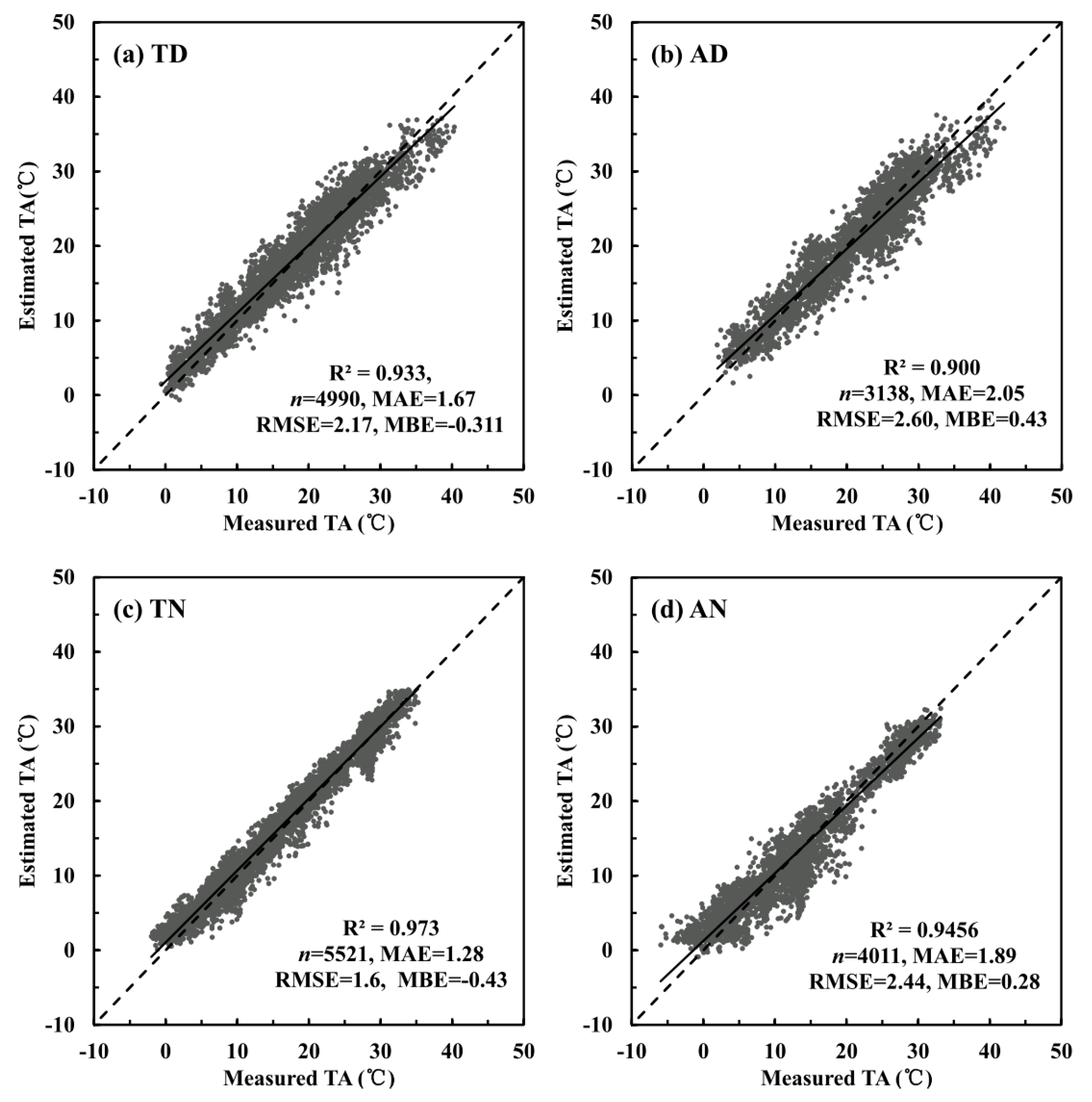
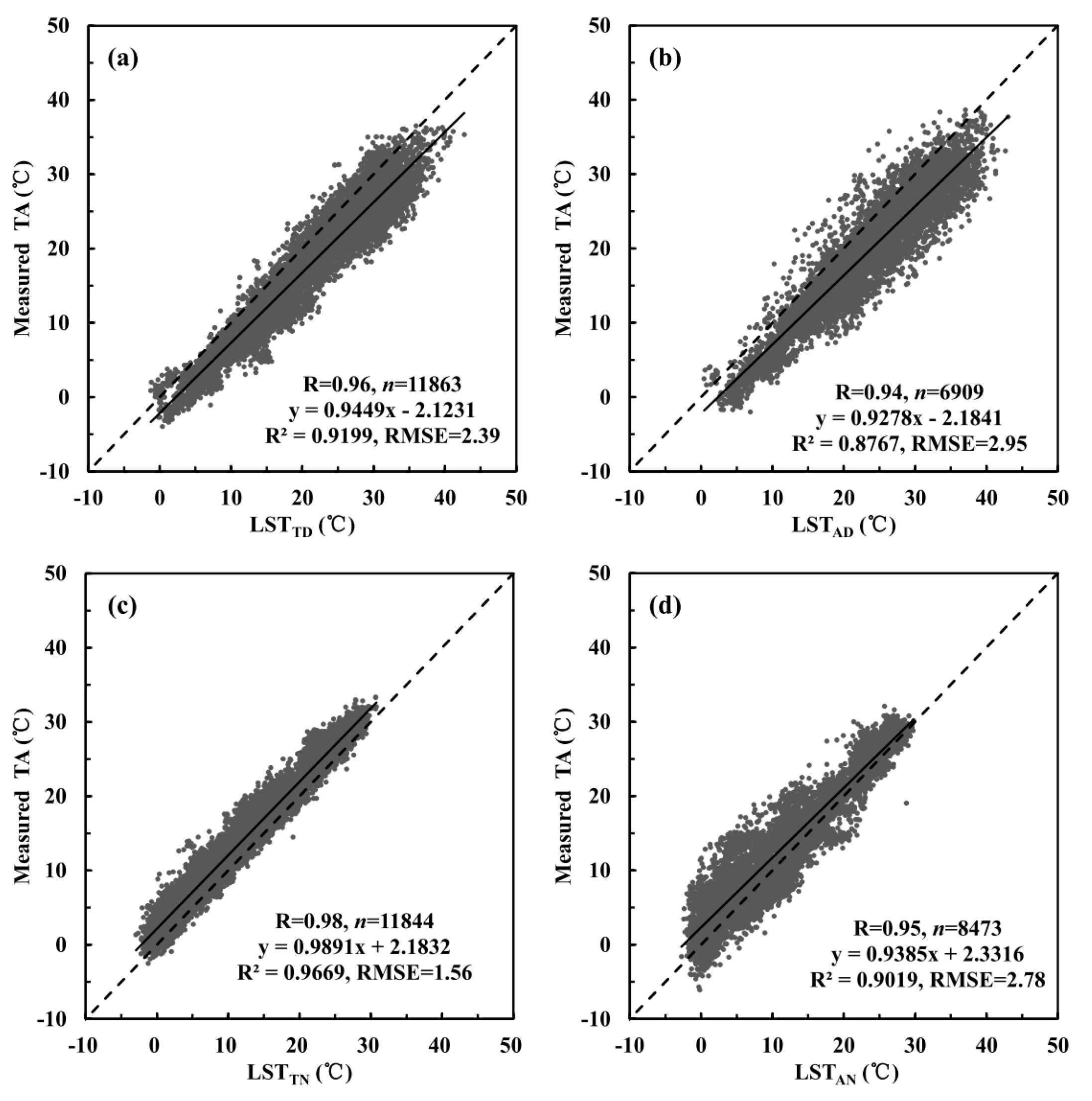
3.1. Calibration and Validation of the Air Temperature Estimation Models Based on Terra/Aqua MODIS

Figure 4 shows the relationships between the observed TA obtained from meteorological stations and the LST derived from both Terra and Aqua satellites. It is obvious that the observed TA and MODIS LST are highly correlated with R greater than 0.9, indicating that LST can provide useful information for estimating TA. Although LST and TA are highly correlated, there are still some variations of TA that cannot be explained by LST without the calibration making use of more predictors. The difference between TA and LST is mainly influenced by the surface energy balance, which is a complex system dependent on factors such as solar radiation, land cover, and soil moisture. Thus, four auxiliary variables including EVI, NDWI, SZA, and DTC were taken into account for calibration of the TA estimation models.
In this study, stepwise linear regression was applied to estimate air temperature. In order to match ground-based TA data with the corresponding satellite data, all the corresponding data values of the independent variables including LST, EVI, NDWI, SZA, and DTC were extracted from images according to meteorological stations’ coordinates. The training dataset during the period 2006–2011 (containing n = 11,863, 11,844, 6909, and 8473 samples with cloud-free pixels, belonging respectively, to daytime and nighttime satellite passes of Terra from 2006 to 2011 and Aqua from 2006 to 2011) was used for model calibration. The remaining dataset during the period 2012–2013 (containing n = 4990, 3138, 5521, and 4011 samples with cloud-free pixels, belonging respectively, to daytime and nighttime satellite passes of Terra and Aqua from 2012 to 2013) was used for model validation. According to the calibration dataset, the statistical equations for air temperature at the four overpass times were constructed by stepwise linear regression using SPSS, and all equations were statistically significant at the 99% confidence level (Table 2).
Figure 5 shows the scatter plots between the measured TA from meteorological stations and estimated TA from the stepwise linear regression model based on validation dataset. It is obvious that most of the points were distributed around the line 1:1. This indicates a good agreement between the estimated and measured TA. The MAE values of TATD, TAAD, TATN, and TAAN estimation models are all lower than 2 °C, and the MBE values are −0.31, 0.43, −0.43, and 0.28 °C for TATD, TAAD, TATN, and TAAD estimation models, respectively. Moreover, the R2 values are all greater than 0.90. The RMSE values are 2.17, 2.60, 1.61, and 2.44 °C for TATD, TAAD, TATN, and TAAD estimation models, respectively. It is evident that TA estimated from satellite measurements is more accurate at nighttime, when differential surface heating is absent and the correlation between surface temperature and air temperature is stronger [14,52,57,58].
The analysis of UHI intensity in the canopy layer requires the computation of air temperatures in the urban and reference rural area. Using slightly more precise regression models, air temperatures at the four different overpass times were computed using the corresponding algorithms in Table 2 for each daytime and nighttime scene during the period 2000–2013. The monthly CUHI climatology maps over Shanghai were produced based on daily CUHI calculated from Terra/Aqua MODIS-estimated TA during the period 2000–2013. The 1 km resolution of the Terra/Aqua MODIS-derived CUHI climatology maps ensures an adequate spatial coverage of Shanghai, providing data even where corresponding ground-based measurements were not available.

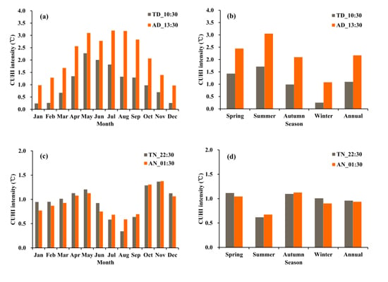
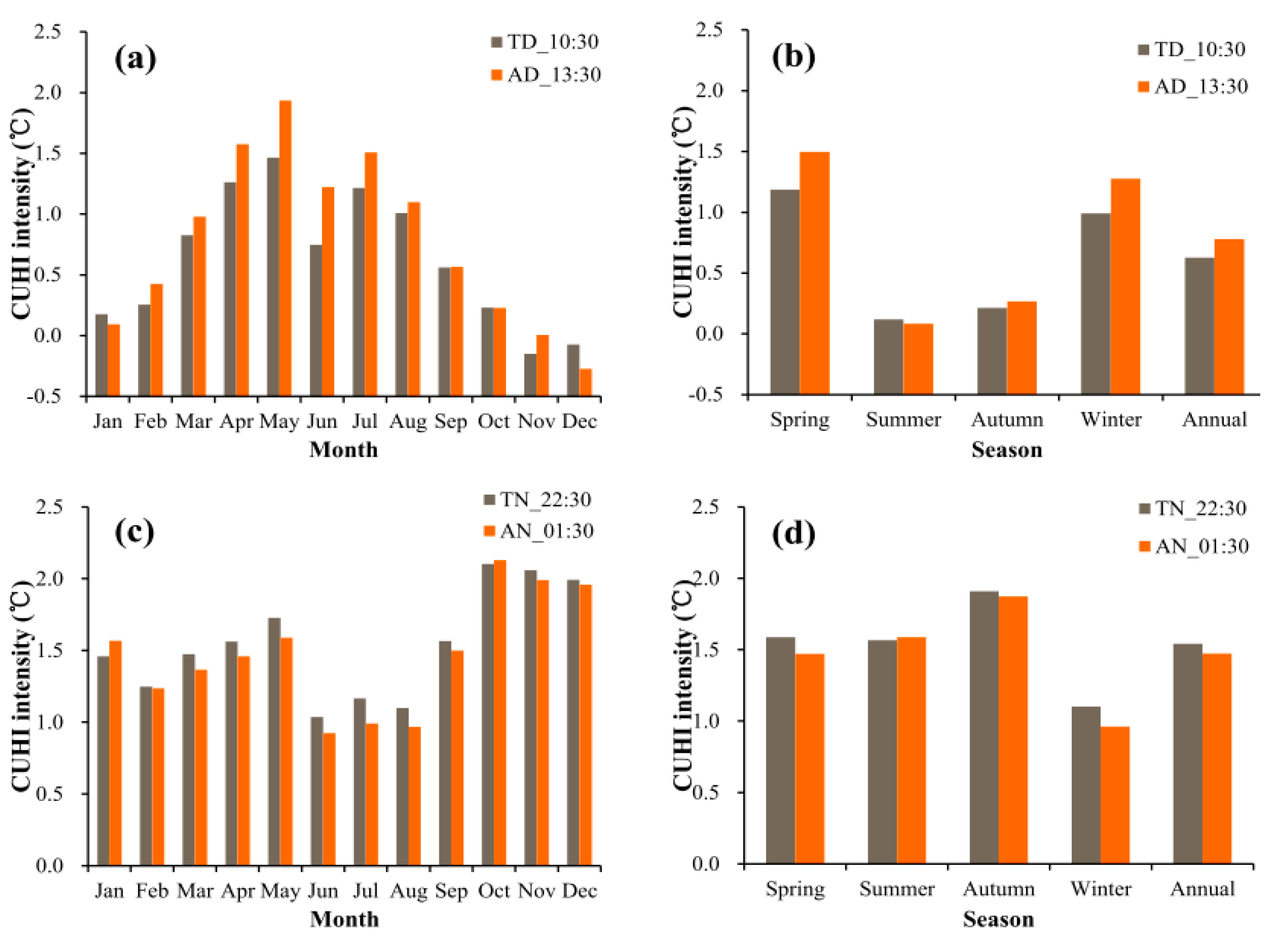
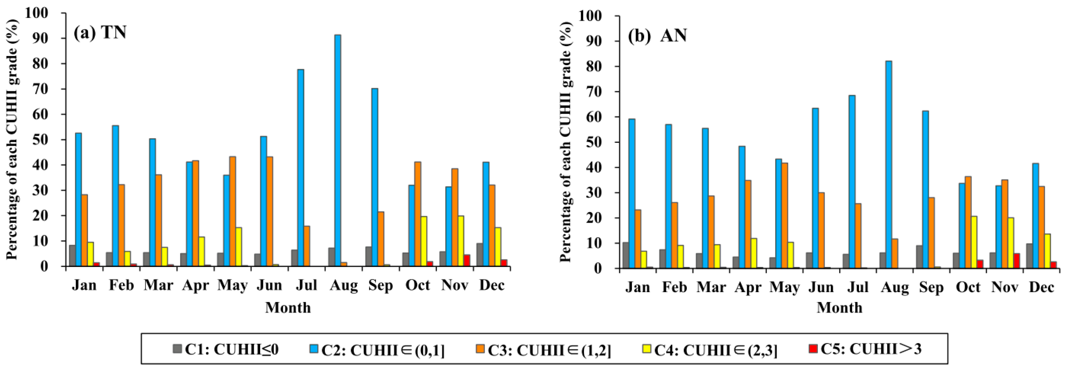
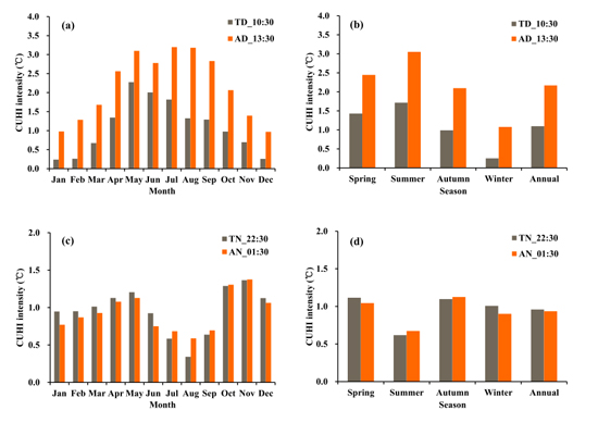
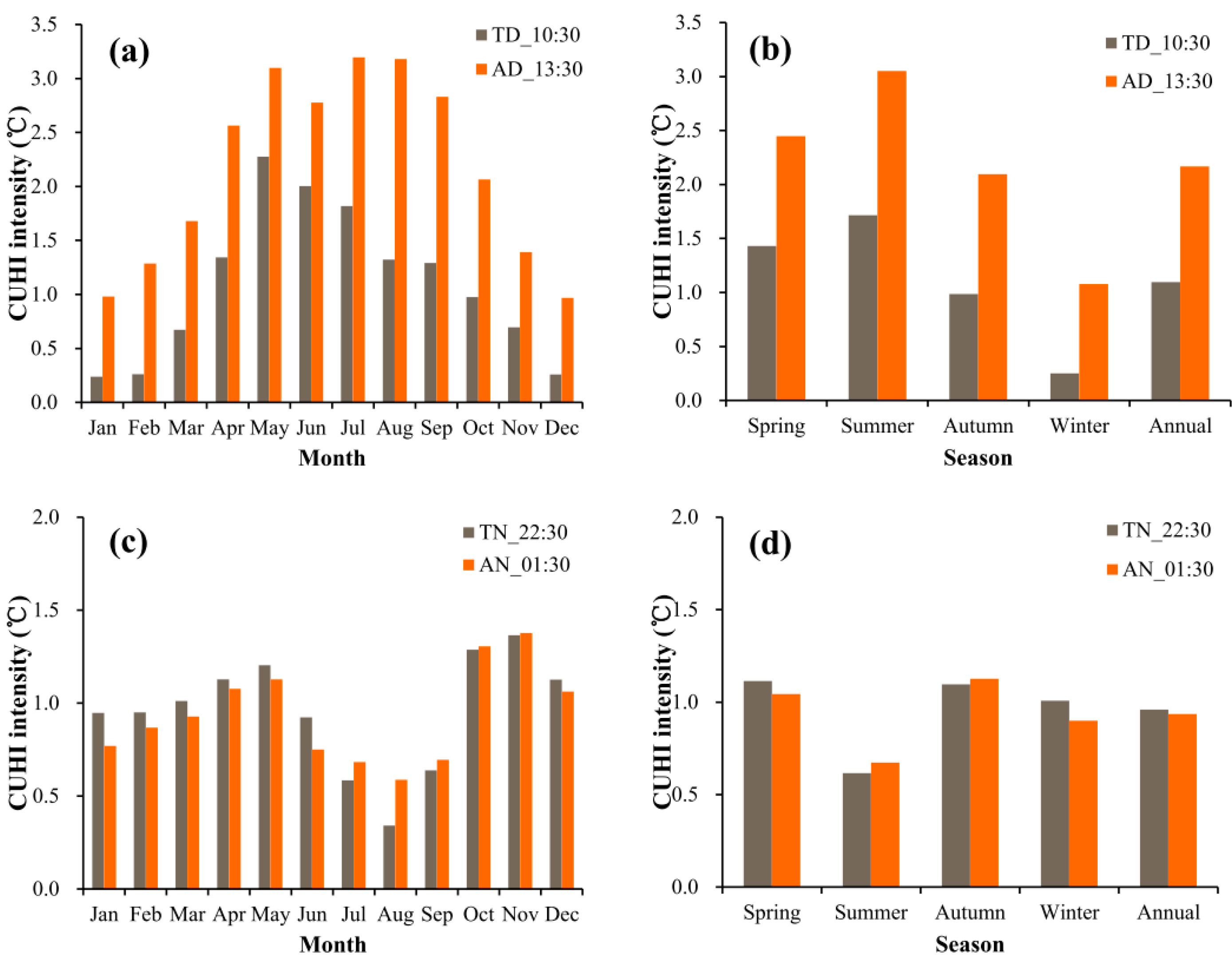
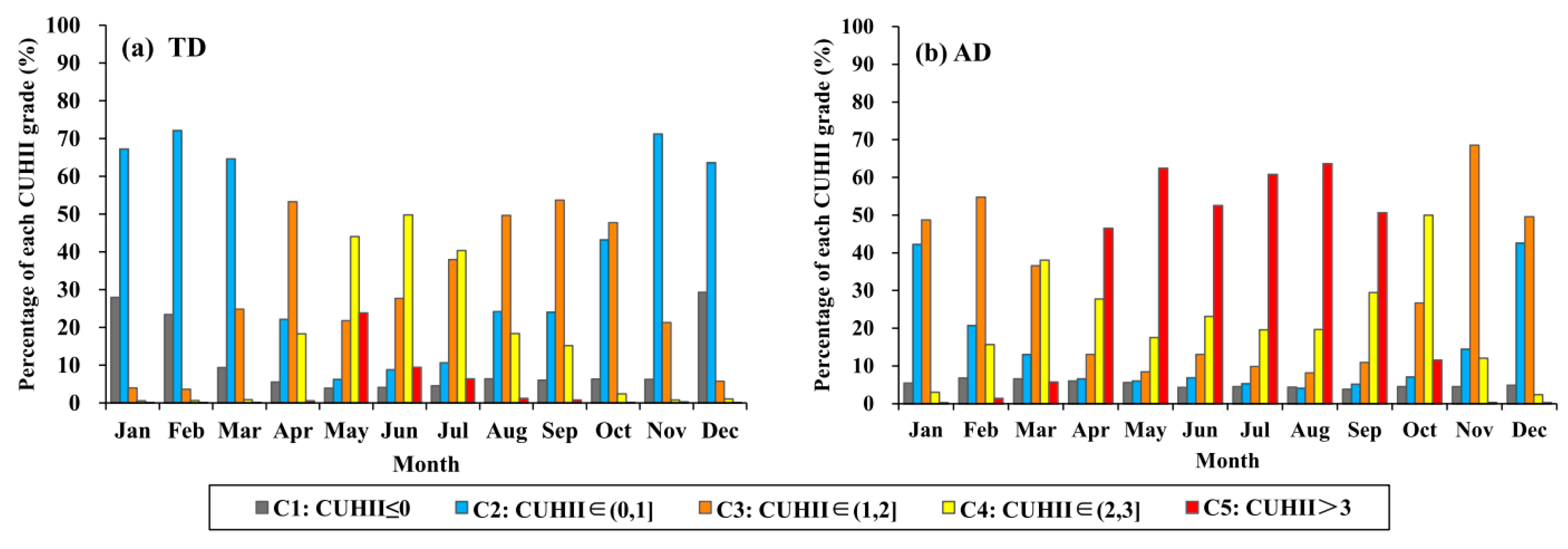
3.2. Temporal Variation of CUHI Intensity Based on Air Temperature Estimated from Terra/Aqua MODIS

3.2.1. Daytime CUHI Climatology

Figure 6a,b shows the monthly and seasonal mean daytime CUHI intensity detected at the Terra and Aqua overpass times during the period 2000–2013. The monthly CUHI intensity is a spatial average value for the urban areas in Shanghai. As shown in Figure 6b, the annual mean daytime CUHI intensity for the Terra overpass time from 2000 to 2013 is 1.1 °C, with a CUHI intensity maximum in summer (1.7 °C). It is obvious that the daytime CUHI intensity is stronger in spring and summer than in autumn and winter. The monthly mean CUHI intensity varied from 0.2 (January) to 2.3 °C (May). The slightly higher CUHI intensity was found from May to July, with values ranging from 1.8 to 2.3 °C. The highest CUHI intensity occurred in May, with a monthly mean of 2.3 °C.
Figure 6b shows the annual mean daytime CUHI intensity (2.2 °C) for the Aqua overpass time from 2002 to 2013 is slightly higher than that for the Terra overpass time. The maximum seasonal CUHI intensity from Aqua is recorded in summer (3.1 °C), which is 1.4 °C higher than that from the Terra overpass. The daytime CUHI intensity for the Aqua overpass time shows similar seasonal and monthly variations with that for Terra, with stronger daytime CUHI intensities in spring and summer than in autumn and winter. These seasonal variations in CUHI intensity have also been observed in studies by Deng et al. [39] and Zhang et al. [42]. The monthly mean CUHI intensity for the Aqua daytime overpass varied from 1.0 (December) to 3.2 °C (July). Stronger daytime CUHI intensity appeared from May to September, with values ranging from 2.8 to 3.2 °C. The highest CUHI intensity occurred in the summer month of July, with a monthly average of 3.2 °C. This seasonal variation of daytime CUHI intensity is attributable mainly to higher levels of solar energy absorbed by building materials during the day in summer. Conversely, the urban–rural contrast is generally weaker during winter because solar energy absorption is lower and hence there is less energy to be reradiated, despite higher levels of anthropogenic space heating.
There are four explanations for the seasonal variability in daytime CUHI in Shanghai. Firstly, the seasonal variability in daytime CUHI might be due to the variation in the amount of solar radiation received during different seasons, which leads to differentials in landscape thermal inertias by day couple with the anthropogenic heat. Secondly, the surface heat release efficiency is reduced because of reflection and absorption by the urban canopy. Thirdly, there is less energy loss due to latent heat evaporation from impervious urban surfaces, in contrast to the cropland and forest with higher soil moisture in the rural areas. Fourthly, due to relatively higher moisture in rural areas (covered by a lot of paddy rice fields) that restrict the rise in air temperature, the cooling effect was strongest in the rural area in the summer daytime. Finally, with a humid climate in Shanghai, the strongest daytime CUHI was found in summer due to lower convention efficiency in the wet climate where high temperature effects are already compounded by high air humidity [85].
Figure 7a,b shows the monthly and seasonal mean daytime CUHI intensity defined as the air temperature difference between Xujiahui and Fengxian meteorological stations at the corresponding Terra and Aqua overpass time. Comparison with Figure 6a,b shows that the pattern of the satellite-based CUHI is similar to the ones based on the urban and rural weather stations, though slightly higher throughout the year. This is due to the fact that CUHI measured by meteorological stations is calculated from all weather conditions, and the CUHI derived from the satellite is calculated under clear-sky conditions. The results indicate that the daytime CUHI measured by MODIS data at the Terra and Aqua overpasses are valid for revealing seasonal variations.

3.2.2. Nighttime CUHI Climatology

Figure 6c,d shows the monthly and seasonal mean nighttime CUHI intensity detected at the Terra and Aqua overpass during the study period 2000–2013. The 14-year average of nighttime CUHI intensity for the Terra overpass in Shanghai is 1.0 °C, with a minimum CUHI intensity of 0.6 °C in summer. The seasonal mean nighttime CUHI intensity in spring has almost the same value as that in autumn, about 1.1 °C. In addition, nighttime CUHI intensity shows different trends from the daytime CUHI intensity, with the weakest CUHI in summer over the Shanghai metropolitan area. The monthly mean CUHI intensity for the Terra nighttime overpass varied from 0.3 °C (August) to 1.4 °C (November). The slightly higher CUHI intensity was found in the winter months of October and November with values of 1.3 to 1.4 °C, respectively.
Figure 6c,d shows the annual mean nighttime CUHI intensity (1.0 °C) for the Aqua overpass from 2002 to 2013 is almost the same as that for the Terra overpass. The seasonal maximum CUHI intensity appeared in autumn (1.1 °C), which is similar to that for the Terra overpass. The nighttime CUHI intensity for Aqua shows similar seasonal and monthly variations to Terra as shown in Figure 6c,d. The monthly mean CUHI intensity for the Aqua overpass varied from 0.6 °C (August) to 1.4 °C (November). A more intensive CUHI occurred in the winter months of October and November with monthly means of 1.3 to 1.4 °C, respectively.
The seasonal variation of nighttime CUHI is mainly attributable to differences in weather conditions. In Shanghai, wind speed and cloudiness are lowest in autumn, a time in which CUHI intensity is strongest. Additionally, as the highest wind speeds and amount of cloudiness are recorded in summer, the air is convectively unstable, which enhances the mixing of urban and rural air masses that produce the weakest CUHI intensity recorded in summer. Previous studies have indicated that the frequent rainfall events and the unstable lower atmosphere characteristic of monsoon nights might be responsible for the smallest CUHI recorded in summer [86]. In recent years, the Shanghai metropolis has been frequently enveloped by heavy haze especially during winter and spring [87]. The biogeochemical effect of urban aerosol or haze pollution is also a contributing factor to nighttime CUHI [88].
To confirm the accuracy of nighttime CUHI measured by satellite-estimated air temperatures, the ground-based monthly and seasonal mean nighttime CUHI intensities were calculated from the Xujiahui and Fengxian meteorological stations at the corresponding Terra and Aqua overpass times (Figure 7c,d). Comparison with Figure 6c,d shows that the seasonal patterns of satellite-derived CUHI are similar to ground-based CUHI observations at nighttime, though slightly lower throughout the year. This is equally because CUHI measured by meteorological stations are based on point measurements or discrete values, whereas satellite-derived CUHI intensities are based on spatially-averaged or continuous values. At nighttime, the cooling rate in urban areas with green vegetation is almost the same as that in rural areas. As a result, a spatially-averaged CUHI based on MODIS-estimated air temperature is slightly lower than that from ground meteorological stations. These results also indicate that nighttime CUHI intensities measured by MODIS data at the Terra and Aqua overpasses are valid for revealing seasonal variations.

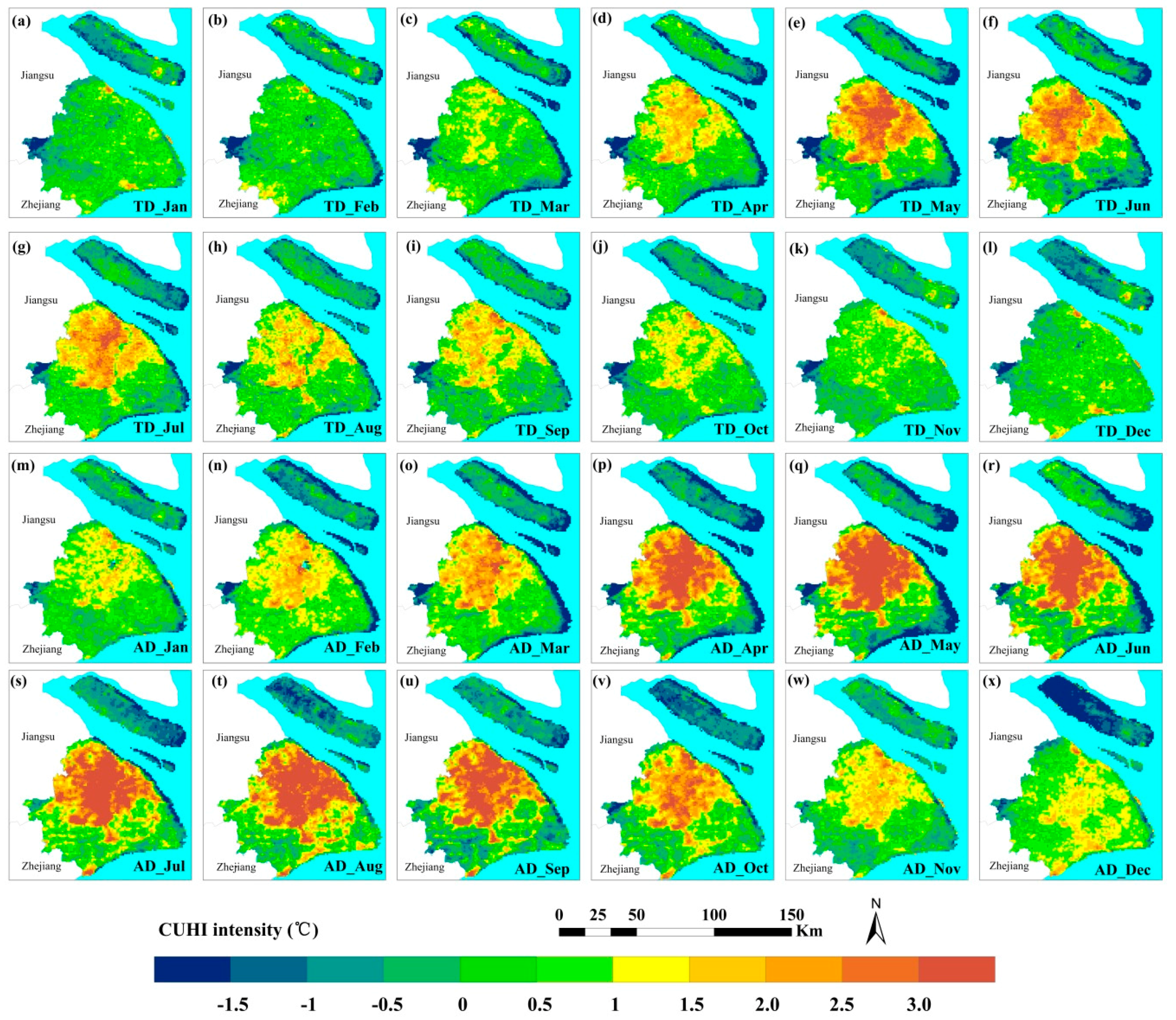
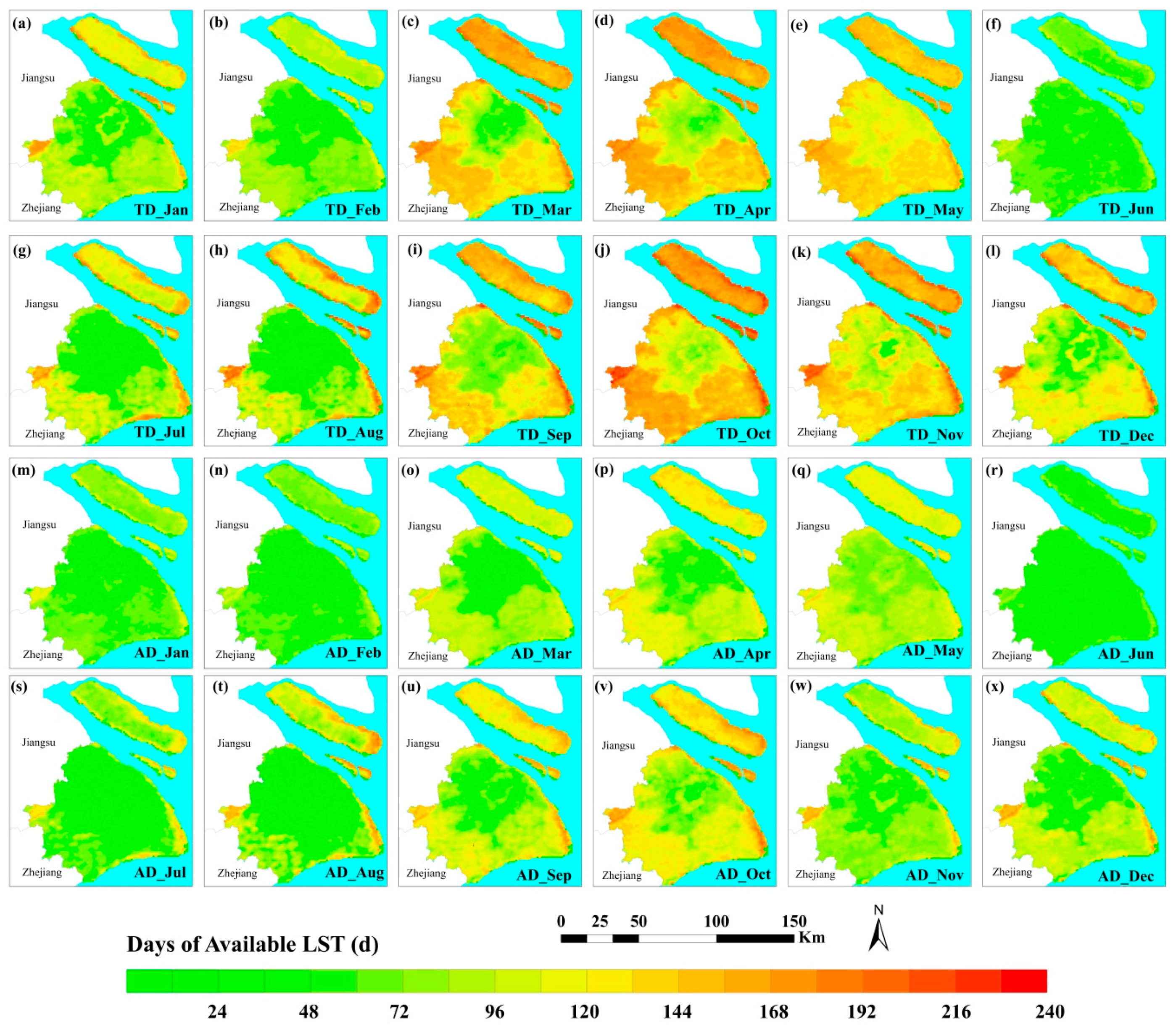
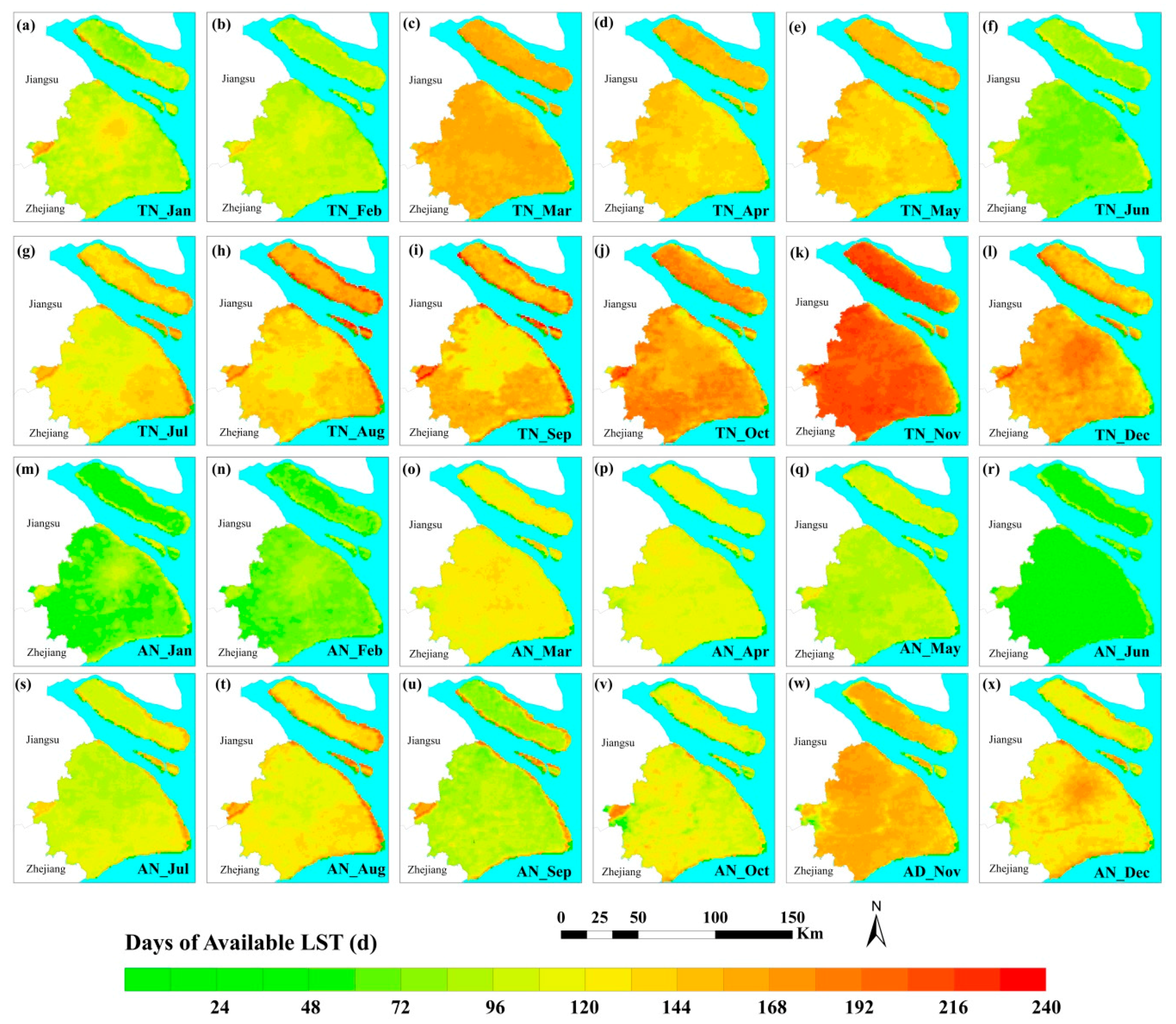
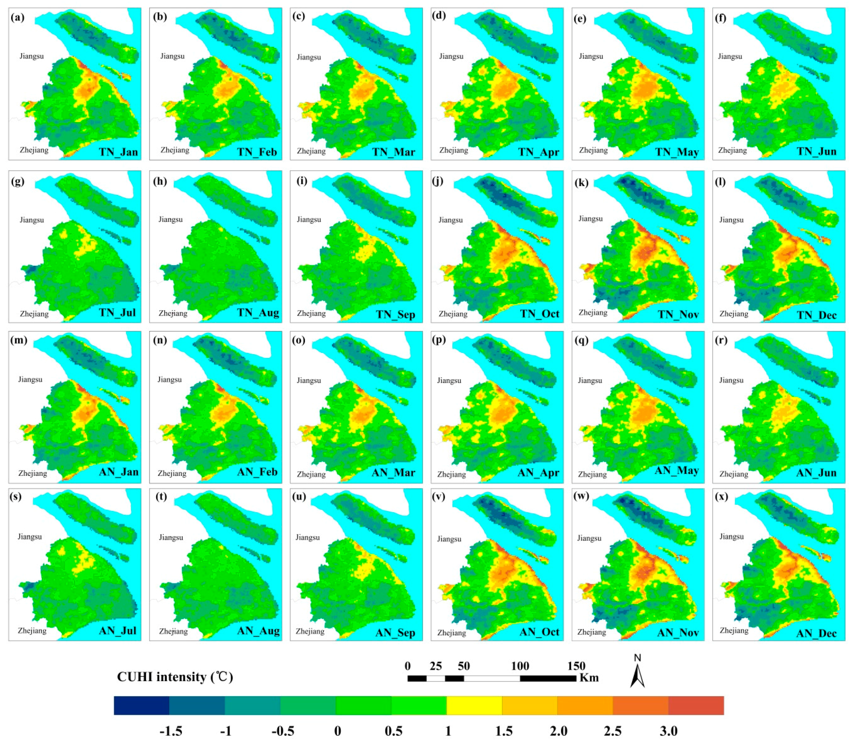
3.3. Spatial Variation of CUHI Intensity Based on Air Temperature Estimated from Terra/Aqua MODIS

Figure 8 show the spatial distribution of monthly mean CUHI intensity averaged from 2000 to 2013 at two daytime overpasses of MODIS (Terra MODIS and Aqua MODIS). To better describe the spatial variability in CUHI intensity obtained from time-series MODIS data over several years, the CUHI intensity was divided into five levels as follows using a threshold value. Three bins were defined by increments of 1 °C between 0 and 3 °C and another two bins with values that were less than 0 °C and higher than 3 °C. According to Figure 8, the area percentage of each CUHI intensity level is calculated for each month at the daytime overpasses of Terra/Aqua as shown in Figure 9.
Figure 8a–l shows the spatial distribution of monthly mean daytime CUHI intensity over Shanghai for Terra daytime overpass during the period 2000–2013. As shown, both the intensity and extent of CUHI varied remarkably depending on the different seasons and accompanying land cover types. The higher CUHI intensity was mainly located in the central urban area and major towns in late spring and summer. In addition, CUHI in the northeastern part of Shanghai, where Baoshan Iron and Steel Corporation is located, shows a higher intensity compared to other areas throughout the year. As shown in Figure 8a–l and Figure 9a, in the spring month of March, the CUHI intensity is relatively weak in most parts of the urban area, and stronger CUHI intensities greater than 2 °C account for 1.1%, which appeared in northeastern Shanghai. Daytime CUHI starts increasing in intensity and spatial extent in late spring and summer, with area percentages of CUHI intensities greater than 2 °C of 67.9%, 59.2%, and 46.8% for May, June and July, respectively. High CUHI intensities (>2 °C) are mainly located at middle sections of the Huangpu River, areas which are economically developed and densely populated. Other parts of this river, along relatively less developed and sparsely populated areas, also exhibit low CUHI intensities due to the significantly smaller air temperature values of water bodies as compared to urban impervious surfaces. In autumn, daytime CUHI intensity experiences a considerable decrease as the area percent of CUHI intensity above 2 °C declined to 16.0%, 2.6%, and 1.1% in September, October, and November, respectively. At this time, a larger portion of the urban area is characterized by weak CUHI intensities. Winter had the lowest seasonal mean CUHI intensity, with most parts in the central urban being less than 1 °C. Only about 1% of the urban area had CUHI intensities greater than 2 °C which can mostly be seen in the Baoshan Iron and Steel Corporation in the northeast, and the Spark Development Zone of Fengxian District in southern Shanghai.
Figure 8m–x shows the spatial distribution of monthly mean daytime CUHI intensity for the Aqua daytime overpass during the period 2002–2013. For the Aqua daytime overpass, the CUHI intensity shows similar seasonal spatial patterns to that of the Terra daytime overpass. However, the Aqua daytime CUHI is larger than the Terra-daytime CUHI in terms of maximum intensity and spatial extent due to differential heating between satellite overpasses. As indicated in Figure 8m–x and Figure 9b, the relatively stronger CUHI intensities (>3 °C) are observed in May, June, July, and August, with monthly area percentages of 62.4%, 52.5%, 60.8%, and 63.7%, respectively. A well defined island shape is clearly evident from May to September, confirming that, urban heating is not an occasional but consistent phenomenon over Shanghai. Higher CUHI intensities often occur in the following areas: (1) the central urban area and the urban fringes along the outer ring road which includes Wusongkou Industrial Park, Huajing Town, Hongqiao Town and Caohejing Town; (2) the major satellite towns with intensive industrial parks or economic development zones in the suburban districts of Pudong, Baoshan, Jiading, Songjiang, and Minghang; and (3) national, district, or township level development zones such as Zhangjiang High-Tech Park, Jinqiao Export Processing Zone (EPZ), and Waigaoqiao Freee Trade Zone (FTZ) in Pudong new area, Minghang Economic and Technical Development Zone (ETDZ), Songjiang EPZ, Jiading Automobile Industrial Zone, and Baoshan Development Zone. Some small spots with low CUHI intensities are detected in the central urban area, which may partly be attributed to the well-preserved Jiangwan wetland, Gongqin forest park, Shanghai plant garden, Xijiao park and emerging patches of green spaces. The area percentage of strong CUHI gradually decreases during the autumn and winter seasons. In the winter months of December and January, the CUHI intensity is weaker, with 2.7% and 3.3% of the urban area being more than 2 °C. The weak CUHI makes up over 90% of urban pixels.
Figure 10a–l shows the spatial distribution of monthly mean nighttime CUHI intensity for the Terra overpass during the period 2000–2013. According to Figure 10, the area percentage of each CUHI intensity level is calculated for each month at the nighttime overpasses of Terra/Aqua as shown in Figure 11. Compared with daytime CUHI intensity, nighttime CUHI is smaller in magnitude and spatial extent. The higher CUHI intensities often appear in the seven districts of the central urban area: Yangpu, Jingan, Hongkou, Xuhui, Huangpu, Changing, and Putuo. In addition, nighttime CUHI intensity shows a different seasonal trend, with the lowest CUHI intensity in summer and highest in autumn. As illustrated in Figure 10a–l and Figure 11a, during spring, a low CUHI intensity (<1 °C) accounts for 55.7%, 46.2%, and 41.2% in March, April, and May, respectively. A higher CUHI intensity (>2 °C) accounts for 8.1%, 12%, and 15.5% in March, April and May, respectively. During summer nights, the CUHI intensity shows its minimum value, with more than 70% of the urban area being below 1 °C. In the autumn months of October and November, the CUHI intensity becomes stronger and the area percentage of CUHI intensity greater than 2 °C increase to 21.6% and 24.4%. In winter nights, the CUHI intensity is slightly weaker than that in autumn.
Figure 10m–x shows the spatial distribution of monthly nighttime mean CUHI intensity at the Aqua overpass during the period 2002–2013. The spatial pattern of Aqua nighttime CUHI intensity is similar to that of Terra, with relatively higher CUHI intensities occurring in northern Shanghai and in the old central urban area including the seven districts. The nighttime CUHI intensity difference between the Aqua and Terra overpass time is insignificant. It shows quite similar seasonal trends to the Terra overpass time, with the lowest CUHI intensity in summer and highest in autumn. As given in Figure 10m–x and Figure 11b, in spring, weak CUHI intensity (<1 °C) accounts for 61.4%, 52.9% and 47.5% in March, April and May, respectively. Stronger CUHI intensity (>2 °C) on the other hand accounts for 9.9%, 12.2% and 10.7% in March, April and May, respectively. At summer nights, CUHI intensity is weakest, with more than 70% of the urban area below 1 °C. In the autumn of October and November, CUHI intensity becomes stronger, with the area percentage of CUHI intensity greater than 2 °C increasing to 23.9% and 26% for the respective months. At winter nights, CUHI intensity is slightly weaker than that in autumn.

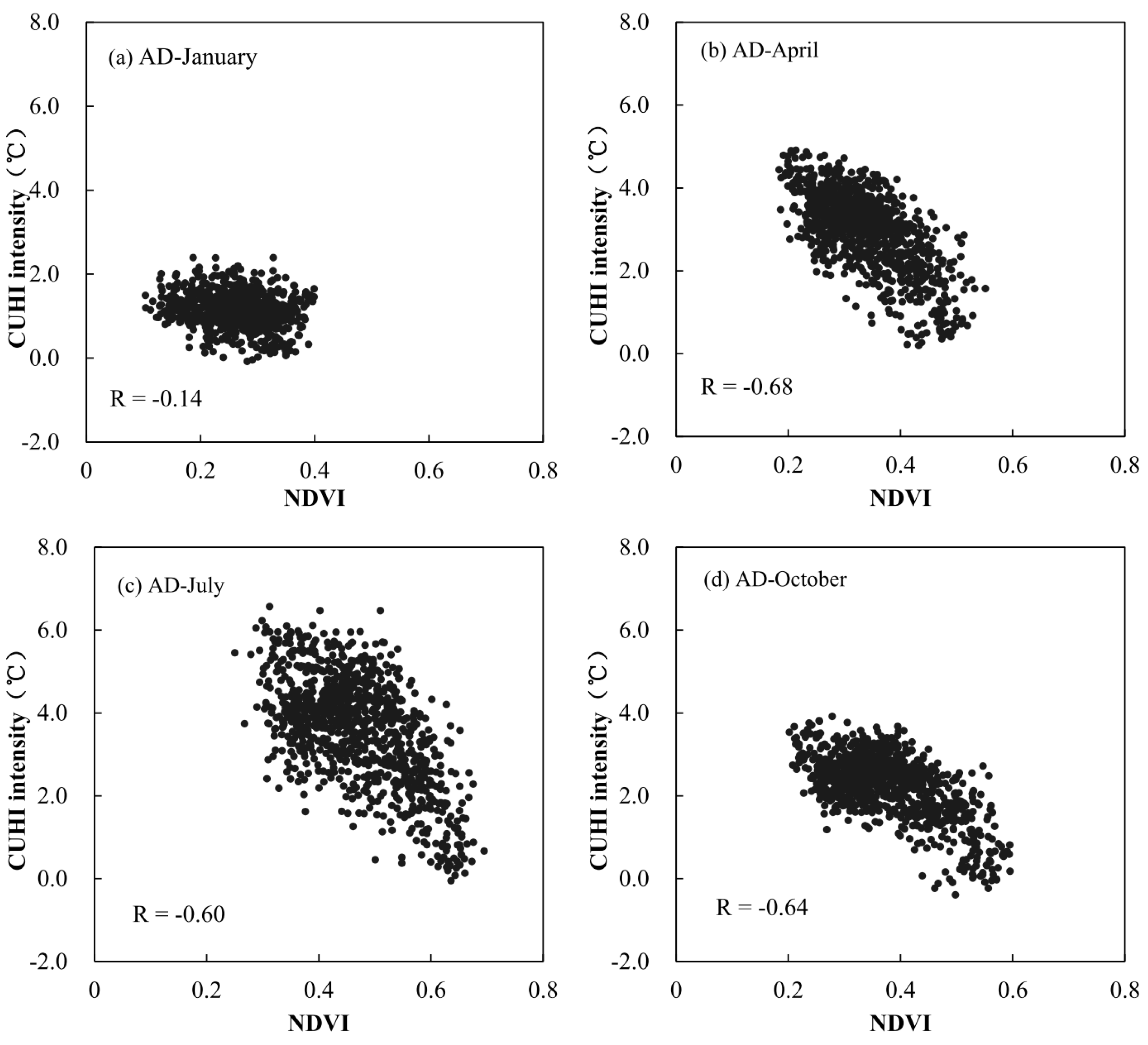
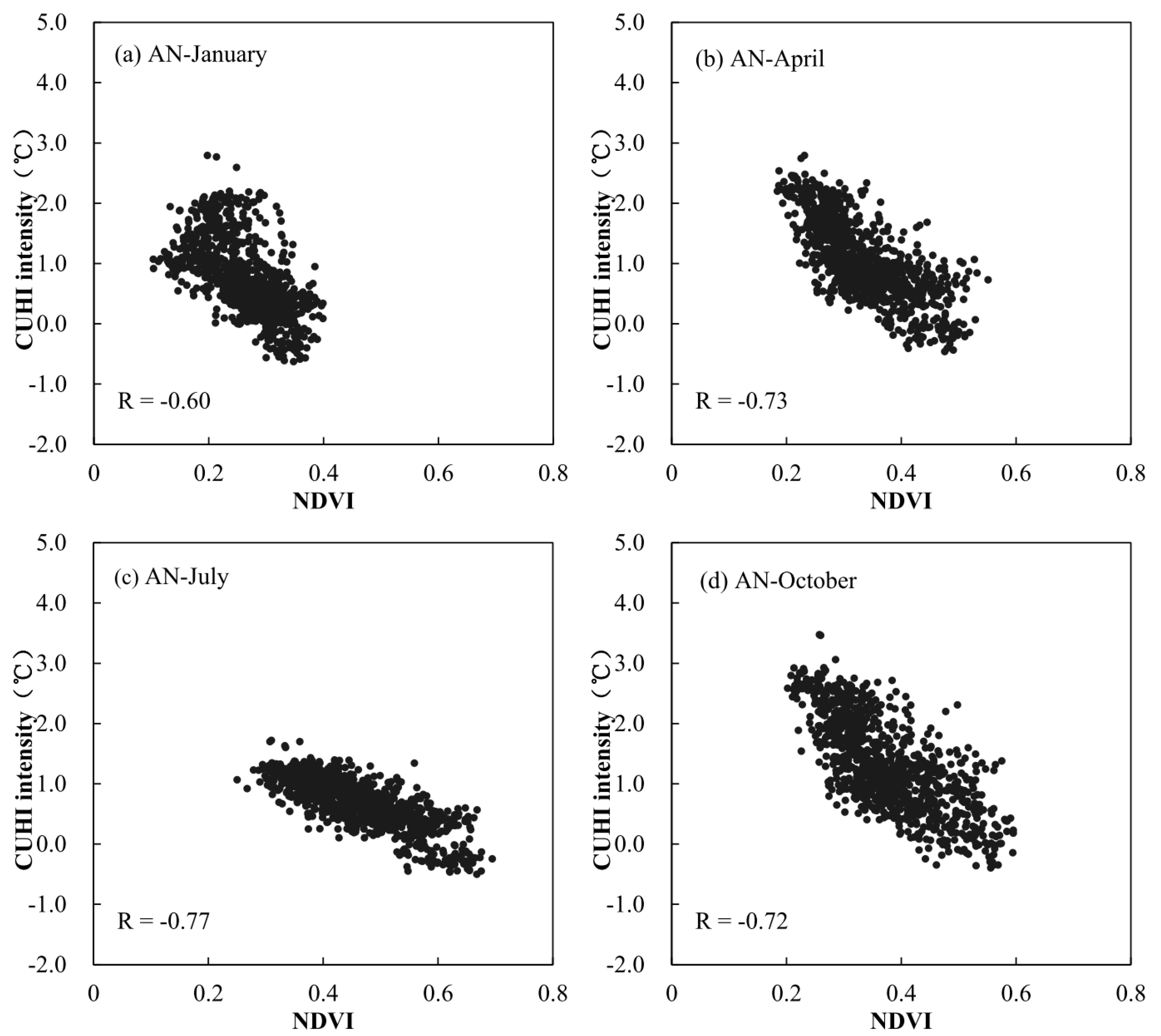
3.4. The Relationship between CUHI Intensity and NDVI

Previous studies have shown that green vegetation can mitigate the urban heat island effect, as vegetation albedo is higher than that of some urban materials such as asphalt surfaces. Moreover, plants use a proportion of the absorbed energy for their life processes, and they tend to cool the surface and the air in their proximity by producing shade and releasing water vapor [89]. In the following, the relationship between CUHI intensity and NDVI is investigated. NDVI is widely used as a proxy for monitoring vegetation health and abundance and it is a significant indicator of the urban climate [90], together with other indices such as those of vegetation fraction [91] and impervious surfaces [47].
The monthly mean CUHI intensity of January, April, July and October representing the four seasons (winter, spring, summer, and autumn, respectively) during the period 2000–2013 were selected to compare with the corresponding monthly mean NDVI (Figure 12 and Figure 13). The scatterplot of daytime CUHI intensity vs. NDVI is shown in Figure 12 and nighttime CUHI intensity vs. NDVI in Figure 13. For each plot, the comparison has been performed with pixels within a square plot of 35 × 35 km in the central urban area (centers at People’s Square). As Figure 12 and Figure 13 indicated, the relationship between CUHI intensity and NDVI varied depending on different seasons for both daytime and nighttime. The daytime figures have similar linear patterns with those of nighttime in the spring, summer and autumn seasons. In the winter month of January, a strong correlation is found between CUHI intensity and NDVI at nighttime, while a weaker correlation between CUHI intensity and NDVI is observed at daytime. An irregular and highly compacted pattern with low NDVI values is shown in the scatterplot for the winter month (January) at daytime. As shown in Figure 12 and Figure 13, pixels with lower CUHI intensity have generally higher NDVI values, and the strong negative correlation between CUHI intensity and NDVI is confirmed in the city center. The highest correlation is found for April at daytime and for July at nighttime, while the correlation decreases in January. Our results were consistent with the trend found in previous study investigating the relationships between LST and NDVI [47,92]. These results suggest that green vegetation can mitigate UHI effects during summer and early autumn. The relatively higher revisit cycle of MODIS allows us to take advantage of the four daily overpasses of Aqua and Terra satellites to study the relationship between the daytime and nighttime CUHI and surface properties.

4. Discussion

As is widely known, Terra/Aqua MODIS offers a great opportunity for environmental monitoring at finer temporal scales. These data have already been tested in urban heat island investigations [21,50]. However, specific applications of these data in mapping CUHI climatology over Shanghai are yet to be undertaken. In this study, we have combined MODIS data with weather station data to estimate spatially continuous air temperature, and a 14-year (2000–2013) data set of daytime and nighttime CUHI climatology in Shanghai is produced in order to evaluate CUHI seasonal variability and spatial distribution.
In our study, we used the spatially continuous air temperature estimated from MODIS LST to produce the CUHI climatology maps, which improved the spatial coverage compared to traditional measurements from meteorological stations and provided the detailed CUHI spatial extent for urban planning and management. Most previous studies in Shanghai barely describe the fine-resolution structure of the CUHI in urban areas due to insufficient spatial density and coverage of weather stations [38,39,40,41,42,61]. In addition, CUHI intensity often varies depending on the choice of urban and rural stations. Some previous studies have used administrative boundaries to classify urban and rural stations without consideration of land surface properties. The environment of meteorological stations are constantly changing and some rural stations as defined in previous studies can no longer be regarded as rural at present due to the rapid urban sprawl in the Shanghai metropolitan area, which may give rise to underestimates of the UHI effect [93].
The CUHI climatological analysis indicates that the daytime CUHI is stronger in the spring and summer than in autumn and winter. This is supported by the research by Zhang et al. [42], who found out that CUHI is higher in summer and spring and weaker in winter and autumn at 14:00, which is quantified by the accumulated intensities based on 11 meteorological stations. Similarly, Deng et al. [39] studied the characteristics of CUHI based on half-hour air temperatures recorded at automatic weather stations in Shanghai, and found out that daytime CUHI intensity is higher in spring and early summer and lowest in autumn. Some previous studies focused on the spatial patterns of SUHI and the relationship between SUHI and surface biophysical parameters in Shanghai [22,25]. Compared with the corresponding CUHI climatological map in July (Figure 8g), the spatial pattern was consistent with the findings in [22], which evaluated daytime SUHI in Shanghai based on a July 2004 Landsat image. UHI is more pronounced in urban residential areas during summer. This is due to more extreme thermal conditions brought by the combined temperature increase characteristic of the summer season and anthropogenic greenhouse gas emissions from factories, automobiles and refrigeration. However, SUHIs usually exhibit stronger and larger spatial variability than CUHI during daytime. In addition, some spatial difference exists due to the different spatial resolutions between MODIS and TM.
The temporal variations of the Shanghai CUHI effect in urban and suburban areas during the period 1978–2007 was investigated by [41] and their results showed CUHI to be strongest in autumn and weakest in summer. These results are different from our findings, as we observed that daytime CUHI is strongest in summer and weakest in winter, while nighttime CUHI is weakest in summer and strongest in autumn and spring. In our study, the seasonal patterns of daytime and nighttime CUHI intensities are quantified based on instantaneous air temperature at different times of the day corresponding to the four Terra/Aqua overpass times, whereas previous studies quantified CUHI intensity using daily mean air temperatures or monthly mean air temperatures. Thus, different CUHI indicators (e.g., daily maximum, minimum, and daily mean air temperature) result in different results in the same study area. We therefore recommend further investigations that would employ several CUHI indicators in parallel, to clarify the range of possible values of CUHI.
Some limitations in our study should also be mentioned. Firstly, this study focuses on the four different times of day corresponding to the satellite Aqua/Terra overpasses. A time series of satellite images combined with air temperature measurements at more synoptic hours would be helpful to unravel the relationship between LSTs and air temperature, the different indicators for the diurnal cycle and across seasons and under different weather conditions. Secondly, we need to stress that our method provides an estimate of the intensity of clear-sky CUHI but not of the likelihood of its occurrence. The clear-sky CUHI climatology estimated differs to some extent, from the real CUHI climatology that is impacted by the actual weather conditions (e.g., for Shanghai in summer, the daytime CUHI may be weaker in reality). For instance, clouds weaken the air temperature difference between urban and rural surfaces. In addition, CUHI intensity is weaker in precipitation days due to the smaller amplitude of the heating/cooling rate and the difference in heating/cooling between urban and rural areas [86]. Therefore, clouds and precipitation may have complicated the relationship between the estimated and real CUHI. Moreover, we were not able to confirm the data quality of the LST data because we had no access to the raw data that were acquired during the satellite flights. However, we did not encounter obvious flaws in the processed LST values. Finally, it is important to note that our climatological analysis of CUHI in Shanghai is only based on 14 years of satellite data. This is due to the limited historical data archive of MODIS which only commenced operations in the year 2000. However, results obtained in this study could be comparable to those of a corresponding interval in a 30-year climate data set. Methods employed in the current study can also be applied in CUHI climatological analysis of other cities in the world.

5. Conclusions

In this study, a long-term (2000–2013) monitoring of seasonal CUHI from MODIS data is analyzed for Shanghai in eastern China. Although most previous studies on CUHI used ground-based data from weather stations, some of those data are not accurate for detail assessment of air temperature in cities. Besides, it is practically difficult to monitor the spatial variation of CUHI with conventional ground-based (weather stations) methods. Satellite remote sensing has the capability to provide a continuous spatial coverage of the area under investigation and was thus used in this study as it offers an efficient and speedy approach for monitoring the spatiotemporal variation in CUHI over a long period of time.
In this work, satellite-derived climatology maps of CUHI intensity over Shanghai were produced using MODIS-estimated air temperature data. Stepwise regression modeling was applied to estimate daytime and nighttime air temperatures based on time series of Terra/Aqua-MODIS LST and other auxiliary variables including enhanced vegetation index (EVI), solar zenith angle (SZA), distance to coast (DTC) and normalized difference water index (NDWI). The comparison between MODIS-derived and ground measured air temperature suggests an accuracy of 1.6–2.6 °C RMSE for the four different times of day. The results show that the daytime CUHI is strongest in summer and weakest in winter, in contrast to nighttime CUHI, which is weakest in summer and strongest in autumn. The multi-annual mean daytime CUHI intensities are 1.1 and 2.17 °C for Terra and Aqua overpasses, respectively, and the seasonal mean CUHI intensities are 1.4 and 2.5 °C for spring, 1.7 and 3.1 °C for summer, 1.0 and 2.1 °C for autumn, and 0.3 and 1.1 °C for winter, respectively, at the Terra and Aqua overpasses. The multi-annual mean nighttime CUHI intensities are 0.96 and 0.94 °C for Terra and Aqua overpasses, respectively, and the seasonal mean CUHI intensities are 1.11 and 1.04 °C for spring, 0.62 and 0.67 °C for summer, 1.1 and 1.13 °C for autumn, and 1.1 and 0.9 °C for winter, respectively, at the Terra and Aqua overpasses. It can be observed from our results that the amount of green vegetation may contribute to this heat variability, as pointed out by the remarkably high negative correlation between CUHI intensity and NDVI, proving that green areas could influence the CUHI phenomenon even in summer. This study has shown the utility of MODIS in producing CHUI climatology maps for a long time, providing CUHI intensity and spatial extent that are suitable for UHI study on a large-scale for heat hazard assessment.

Acknowledgments

This study was supported by the Agricultural Project for Scientific and Technological Research (APSTR) of Shanghai, China (Grant No. 2011-2-11), and the National Key Research and Development Plan of China (Grant No. 2016FYD0300601). We are grateful to the NASA Land Processes Distributed Active Archive Center (LPDAAC) for making the MODIS data available. In addition, we would like to express our sincere thanks to the anonymous reviewers for their constructive comments.

Author Contributions

Jingfeng Huang conceived the original idea of the study, and designed, organized and supervised the entire investigation; Weijiao Huang collected, processed and analyzed the data, and wrote the article; Jun Li provided meteorological observation data and also assisted in data analysis and preparation of the article; Qiaoying Guo and Xinxing Li assisted in data collection, processing and analysis; and Lamin R. Mansaray provided relevant advice and edited the article.

Conflicts of Interest

The authors declare no conflict of interest.

References

  1. United Nations. World Urbanization Prospects: The 2014 Revision; Department of Economic and Social Affairs, Population Division: New York, NY, USA, 2015; p. 1. [Google Scholar]
  2. Chudnovsky, A.; Ben-Dor, E.; Saaroni, H. Diurnal thermal behavior of selected urban objects using remote sensing measurements. Energy Build. 2004, 36, 1063–1074. [Google Scholar] [CrossRef]
  3. Wang, K.; Wang, J.; Wang, P.; Sparrow, M.; Yang, J.; Chen, H. Influences of urbanization on surface characteristics as derived from the Moderate-Resolution Imaging Spectroradiometer: A case study for the Beijing metropolitan area. J. Geophys. Res. Atmos. 2007, 112, D22S–D26S. [Google Scholar] [CrossRef]
  4. Kolokotroni, M.; Ren, X.; Davies, M.; Mavrogianni, A. London’s urban heat island: Impact on current and future energy consumption in office buildings. Energy Build. 2012, 47, 302–311. [Google Scholar] [CrossRef]
  5. Santamouris, M.; Cartalis, C.; Synnefa, A.; Kolokotsa, D. On the impact of urban heat island and global warming on the power demand and electricity consumption of buildings—A review. Energy Build. 2015, 98, 119–124. [Google Scholar] [CrossRef]
  6. Stathopoulou, E.; Mihalakakou, G.; Santamouris, M.; Bagiorgas, H.S. On the impact of temperature on tropospheric ozone concentration levels in urban environments. J. Earth Syst. Sci. 2008, 117, 227–236. [Google Scholar] [CrossRef]
  7. Sakka, A.; Santamouris, M.; Livada, I.; Nicol, F.; Wilson, M. On the thermal performance of low income housing during heat waves. Energy Build. 2012, 49, 69–77. [Google Scholar] [CrossRef]
  8. Van Hove, L.; Jacobs, C.; Heusinkveld, B.G.; Elbers, J.A.; Van Driel, B.L.; Holtslag, A. Temporal and spatial variability of urban heat island and thermal comfort within the Rotterdam agglomeration. Build. Environ. 2015, 83, 91–103. [Google Scholar] [CrossRef]
  9. Pantavou, K.; Theoharatos, G.; Mavrakis, A.; Santamouris, M. Evaluating thermal comfort conditions and health responses during an extremely hot summer in Athens. Build. Environ. 2011, 46, 339–344. [Google Scholar] [CrossRef]
  10. Voogt, J.A.; Oke, T.R. Thermal remote sensing of urban climates. Remote Sens. Environ. 2003, 86, 370–384. [Google Scholar] [CrossRef]
  11. Yang, X.; Hou, Y.; Chen, B. Observed surface warming induced by urbanization in east China. J. Geophys. Res. Atmos. 2011, 116, 1–12. [Google Scholar] [CrossRef]
  12. Santamouris, M. Heat island research in Europe: The state of the art. Adv. Build. Energ. Res. 2007, 1, 123–150. [Google Scholar] [CrossRef]
  13. Chen, Y.; Sun, H.; Li, J. Estimating daily maximum air temperature with MODIS data and a daytime temperature variation model in Beijing urban area. Remote Sens. Lett. 2016, 7, 865–874. [Google Scholar] [CrossRef]
  14. Pichierri, M.; Bonafoni, S.; Biondi, R. Satellite air temperature estimation for monitoring the canopy layer heat island of Milan. Remote Sens. Environ. 2012, 127, 130–138. [Google Scholar] [CrossRef]
  15. Streutker, D.R. A remote sensing study of the urban heat island of Houston, Texas. Int. J. Remote Sens. 2002, 23, 2595–2608. [Google Scholar] [CrossRef]
  16. Nichol, J. Remote sensing of urban heat islands by day and night. Photogramm. Eng. Remote Sens. 2005, 71, 613–621. [Google Scholar] [CrossRef]
  17. Weng, Q. Thermal infrared remote sensing for urban climate and environmental studies: Methods, applications, and trends. ISPRS J. Photogramm. 2009, 64, 335–344. [Google Scholar] [CrossRef]
  18. Ma, Y.; Kuang, Y.; Huang, N. Coupling urbanization analyses for studying urban thermal environment and its interplay with biophysical parameters based on TM/ETM+ imagery. Int. J. Appl. Earth Obs. 2010, 12, 110–118. [Google Scholar] [CrossRef]
  19. Shen, H.; Huang, L.; Zhang, L.; Wu, P.; Zeng, C. Long-term and fine-scale satellite monitoring of the urban heat island effect by the fusion of multi-temporal and multi-sensor remote sensed data: A 26-year case study of the city of Wuhan in China. Remote Sens. Environ. 2016, 172, 109–125. [Google Scholar] [CrossRef]
  20. Wang, J.; Huang, B.; Fu, D.; Atkinson, P.M.; Zhang, X. Response of urban heat island to future urban expansion over the Beijing-Tianjin-Hebei metropolitan area. Appl. Geogr. 2016, 70, 26–36. [Google Scholar] [CrossRef]
  21. Clinton, N.; Gong, P. MODIS detected surface urban heat islands and sinks: Global locations and controls. Remote Sens. Environ. 2013, 134, 294–304. [Google Scholar] [CrossRef]
  22. Li, J.; Wang, X.; Wang, X.; Ma, W.; Zhang, H. Remote sensing evaluation of urban heat island and its spatial pattern of the Shanghai metropolitan area, China. Ecol. Complex. 2009, 6, 413–420. [Google Scholar] [CrossRef]
  23. Li, Y.; Zhang, H.; Kainz, W. Monitoring patterns of urban heat islands of the fast-growing Shanghai metropolis, China: Using time-series of Landsat TM/ETM+ data. Int. J. Appl. Earth Obs. 2012, 19, 127–138. [Google Scholar] [CrossRef]
  24. Chen, L.; Jiang, R.; Xiang, W. Surface Heat Island in Shanghai and its Relationship with Urban Development from 1989 to 2013. Adv. Meteorol. 2016, 2016, 1–15. [Google Scholar] [CrossRef]
  25. Li, J.X.; Song, C.H.; Cao, L.; Zhu, F.G.; Meng, X.L.; Wu, J.G. Impacts of landscape structure on surface urban heat islands: A case study of Shanghai, China. Remote Sens. Environ. 2011, 115, 3249–3263. [Google Scholar] [CrossRef]
  26. Zhang, H.; Qi, Z.; Ye, X.; Cai, Y.; Ma, W.; Chen, M. Analysis of land use/land cover change, population shift, and their effects on spatiotemporal patterns of urban heat islands in metropolitan Shanghai, China. Appl. Geogr. 2013, 44, 121–133. [Google Scholar] [CrossRef]
  27. Tran, H.; Uchihama, D.; Ochi, S.; Yasuoka, Y. Assessment with satellite data of the urban heat island effects in Asian mega cities. Int. J. Appl. Earth Obs. 2006, 8, 34–48. [Google Scholar] [CrossRef]
  28. Kataoka, K.; Matsumoto, F.; Ichinose, T.; Taniguchi, M. Urban warming trends in several large Asian cities over the last 100 years. Sci. Total Environ. 2009, 407, 3112–3119. [Google Scholar] [CrossRef] [PubMed]
  29. Gaffin, S.R.; Rosenzweig, C.; Khanbilvardi, R.; Parshall, L.; Mahani, S.; Glickman, H.; Goldberg, R.; Blake, R.; Slosberg, R.B.; Hillel, D. Variations in New York city’s urban heat island strength over time and space. Theor. Appl. Climatol. 2008, 94, 1–11. [Google Scholar] [CrossRef]
  30. Kim, Y.H.; Baik, J.J. Spatial and temporal structure of the urban heat island in Seoul. J. Appl. Meteorol. 2005, 44, 591–605. [Google Scholar] [CrossRef]
  31. Siu, L.W.; Hart, M.A. Quantifying urban heat island intensity in Hong Kong SAR, China. Environ. Monit. Assess. 2013, 185, 4383–4398. [Google Scholar] [CrossRef] [PubMed]
  32. Chow, W.T.L.; Roth, M. Temporal dynamics of the urban heat island of Singapore. Int. J. Climatol. 2006, 26, 2243–2260. [Google Scholar] [CrossRef]
  33. Zhang, J.; Meng, Q.; Li, X.; Yang, L. Urban heat island variations in Beijing region in multi spatial and temporal scales. Sci. Geogr. Sin. 2011, 31, 1349–1354. [Google Scholar]
  34. Yang, P.; Ren, G.; Liu, W. Spatial and temporal characteristics of Beijing urban heat island intensity. J. Appl. Meteorol. Clim. 2013, 52, 1803–1816. [Google Scholar] [CrossRef]
  35. Fortuniak, K.; Kłysik, K.; Wibig, J. Urban–rural contrasts of meteorological parameters in Łódź. Theor. Appl. Climatol. 2006, 84, 91–101. [Google Scholar] [CrossRef]
  36. Papanastasiou, D.K.; Kittas, C. Maximum urban heat island intensity in a medium-sized coastal Mediterranean city. Theor. Appl. Climatol. 2012, 107, 407–416. [Google Scholar] [CrossRef]
  37. Montavez, J.P.; Rodriguez, A.; Jimenez, J.I. A study of the Urban Heat Island of Granada. Int. J. Climatol. 2000, 20, 899–911. [Google Scholar] [CrossRef]
  38. Zhou, S.Z.; Zhang, C. On the Shanghai urban heat island effect. Acta Geogr. Sin. 1982, 37, 372–381. [Google Scholar]
  39. Deng, L.; Shu, J.; Li, C. Character analysis of Shanghai urban heat island. J. Trop. Meteorol. 2001, 3, 9–11. [Google Scholar]
  40. Zhao, S.; Da, L.; Tang, Z.; Fang, H.; Song, K.; Fang, J. Ecological consequences of rapid urban expansion: Shanghai, China. Front. Ecol. Environ. 2006, 4, 341–346. [Google Scholar] [CrossRef]
  41. Zhang, K.; Wang, R.; Shen, C.; Da, L. Temporal and spatial characteristics of the urban heat island during rapid urbanization in Shanghai, China. Environ. Monit. Assess. 2010, 169, 101–112. [Google Scholar] [CrossRef] [PubMed]
  42. Zhang, Y.; Bao, W.J.; Yu, Q.; Ma, W.C. Study on seasonal variations of the urban heat island and its interannual changes in a typical Chinese megacity. Chin. J. Geophys. 2012, 55, 1121–1128. [Google Scholar]
  43. Benali, A.; Carvalho, A.C.; Nunes, J.P.; Carvalhais, N.; Santos, A. Estimating air surface temperature in Portugal using MODIS LST data. Remote Sens. Environ. 2012, 124, 108–121. [Google Scholar] [CrossRef]
  44. Hu, L.; Brunsell, N.A. A new perspective to assess the urban heat island through remotely sensed atmospheric profiles. Remote Sens. Environ. 2015, 158, 393–406. [Google Scholar] [CrossRef]
  45. Ho, H.C.; Knudby, A.; Sirovyak, P.; Xu, Y.; Hodul, M.; Henderson, S.B. Mapping maximum urban air temperature on hot summer days. Remote Sens. Environ. 2014, 154, 38–45. [Google Scholar] [CrossRef]
  46. Oke, T.R.; Maxwell, G.B. Urban heat island dynamics in Montreal and Vancouver. Atmos. Environ. 1975, 9, 191–200. [Google Scholar] [CrossRef]
  47. Yuan, F.; Bauer, M.E. Comparison of impervious surface area and normalized difference vegetation index as indicators of surface urban heat island effects in Landsat imagery. Remote Sens. Environ. 2007, 106, 375–386. [Google Scholar] [CrossRef]
  48. Deng, C.; Wu, C. Examining the impacts of urban biophysical compositions on surface urban heat island: A spectral unmixing and thermal mixing approach. Remote Sens. Environ. 2013, 131, 262–274. [Google Scholar] [CrossRef]
  49. Lazzarini, M.; Marpu, P.R.; Ghedira, H. Temperature-land cover interactions: The inversion of urban heat island phenomenon in desert city areas. Remote Sens. Environ. 2013, 130, 136–152. [Google Scholar] [CrossRef]
  50. Haashemi, S.; Weng, Q.; Darvishi, A.; Alavipanah, S. Seasonal variations of the surface urban heat island in a Semi-Arid city. Remote Sens. 2016, 8, 352. [Google Scholar] [CrossRef]
  51. Xu, Y.; Qin, Z.; Shen, Y. Study on the estimation of near-surface air temperature from MODIS data by statistical methods. Int. J. Remote Sens. 2012, 33, 7629–7643. [Google Scholar] [CrossRef]
  52. Zhu, W.; Lű, A.; Jia, S. Estimation of daily maximum and minimum air temperature using MODIS land surface temperature products. Remote Sens. Environ. 2013, 130, 62–73. [Google Scholar] [CrossRef]
  53. Sun, H.; Chen, Y.; Gong, A.; Zhao, X.; Zhan, W.; Wang, M. Estimating mean air temperature using MODIS day and night land surface temperatures. Theor. Appl. Climatol. 2014, 118, 81–92. [Google Scholar] [CrossRef]
  54. Stisen, S.; Sandholt, I.; Norgaard, A.; Fensholt, R.; Eklundh, L. Estimation of diurnal air temperature using MSG SEVIRI data in West Africa. Remote Sens. Environ. 2007, 110, 262–274. [Google Scholar] [CrossRef]
  55. Janatian, N.; Sadeghi, M.; Sanaeinejad, S.H.; Bakhshian, E.; Farid, A.; Hasheminia, S.M.; Ghazanfari, S. A statistical framework for estimating air temperature using MODIS land surface temperature data. Int. J. Climatol. 2016. [Google Scholar] [CrossRef]
  56. Zhang, H.; Zhang, F.; Ye, M.; Che, T.; Zhang, G. Estimating daily air temperatures over the Tibetan Plateau by dynamically integrating MODIS LST data. J. Geophys. Res. Atmos. 2016, 121, 11425–11441. [Google Scholar] [CrossRef]
  57. Lin, X.; Zhang, W.; Huang, Y.; Sun, W.; Han, P.; Yu, L.; Sun, F. Empirical estimation of Near-Surface air temperature in china from MODIS LST data by considering physiographic features. Remote Sens. 2016, 8, 629. [Google Scholar] [CrossRef]
  58. Huang, R.; Zhang, C.; Huang, J.; Zhu, D.; Wang, L.; Liu, J. Mapping of daily mean air temperature in agricultural regions using daytime and nighttime land surface temperatures derived from TERRA and AQUA MODIS data. Remote Sens. 2015, 7, 8728–8756. [Google Scholar] [CrossRef]
  59. Vancutsem, C.; Ceccato, P.; Dinku, T.; Connor, S.J. Evaluation of MODIS land surface temperature data to estimate air temperature in different ecosystems over Africa. Remote Sens. Environ. 2010, 114, 449–465. [Google Scholar] [CrossRef]
  60. Kim, D.; Han, K. Remotely sensed retrieval of midday air temperature considering atmospheric and surface moisture conditions. Int. J. Remote Sens. 2013, 34, 247–263. [Google Scholar] [CrossRef]
  61. Tan, J.; Zheng, Y.; Tang, X.; Guo, C.; Li, L.; Song, G.; Zhen, X.; Yuan, D.; Kalkstein, A.J.; Li, F.; et al. The urban heat island and its impact on heat waves and human health in Shanghai. Int. J. Biometeorol. 2010, 54, 75–84. [Google Scholar] [CrossRef] [PubMed]
  62. Jarraud, M. Guide to Meteorological Instruments and Methods of Observation (WMO-No. 8); World Meteorological Organisation: Geneva, Switzerland, 2008. [Google Scholar]
  63. Wan, Z.M. New refinements and validation of the MODIS Land-Surface Temperature/Emissivity products. Remote Sens. Environ. 2008, 112, 59–74. [Google Scholar] [CrossRef]
  64. Wan, Z.M.; Dozier, J. A generalized split-window algorithm for retrieving land-surface temperature from space. IEEE Trans. Geosci. Remote Sens. 1996, 34, 892–905. [Google Scholar]
  65. Wan, Z.M. MODIS Land Surface Temperature Products Users’ Guide. Available online: https://icess.eri.ucsb.edu/modis/LstUsrGuide/usrguide.html (accessed on 17 April 2017).
  66. Noi, P.T.; Degener, J.; Kappas, M. Comparison of multiple linear regression, cubist regression, and random forest algorithms to estimate daily air surface temperature from dynamic combinations of MODIS LST data. Remote Sens. 2017, 9, 398. [Google Scholar] [CrossRef]
  67. Friedl, M.A.; McIver, D.K.; Hodges, J.C.F.; Zhang, X.Y.; Muchoney, D.; Strahler, A.H.; Woodcock, C.E.; Gopal, S.; Schneider, A.; Cooper, A.; et al. Global land cover mapping from MODIS: Algorithms and early results. Remote Sens. Environ. 2002, 83, 287–302. [Google Scholar] [CrossRef]
  68. Friedl, M.A.; Sulla-Menashe, D.; Tan, B.; Schneider, A.; Ramankutty, N.; Sibley, A.H.X. MODIS Collection 5 global land cover: Algorithm refinements and characterization of new datasets. Remote Sens. Environ. 2010, 114, 168–182. [Google Scholar] [CrossRef]
  69. Loveland, T.R.; Belward, A.S. The IGBP-DIS global 1 km land cover data set, DISCover: First results. Int. J. Remote Sens. 1997, 18, 3289–3295. [Google Scholar] [CrossRef]
  70. Hansen, M.C.; Defries, R.S.; Townshend, J.; Sohlberg, R. Global land cover classification at 1km spatial resolution using a classification tree approach. Int. J. Remote Sens. 2000, 21, 1331–1364. [Google Scholar] [CrossRef]
  71. Lotsch, A.; Tian, Y.; Friedl, M.A.; Myneni, R.B. Land cover mapping in support of LAI and FPAR retrievals from EOS-MODIS and MISR: Classification methods and sensitivities to errors. Int. J. Remote Sens. 2003, 24, 1997–2016. [Google Scholar] [CrossRef]
  72. Running, S.W.; Loveland, T.R.; Pierce, L.L.; Nemani, R.; Hunt, E.R. A remote-sensing based vegetation classification logic for global land-cover analysis. Remote Sens. Environ. 1995, 51, 39–48. [Google Scholar] [CrossRef]
  73. Bonan, G.B.; Levis, S.; Kergoat, L.; Oleson, K.W. Landscapes as patches of plant functional types: An integrating concept for climate and ecosystem models. Glob. Biogeochem. Cycles 2002, 16. [Google Scholar] [CrossRef]
  74. Ninyerola, M.; Pons, X.; Roure, J.M. A methodological approach of climatological modelling of air temperature and precipitation through GIS techniques. Int. J. Climatol. 2000, 20, 1823–1841. [Google Scholar] [CrossRef]
  75. Oke, T.R. Boundary Layer Climates, 2nd ed.; Methuen: London, UK, 1987; p. 435. [Google Scholar]
  76. Arribas, A.; Gallardo, C.; Gaertner, M.; Castro, M. Sensitivity of the Iberian Peninsula climate to a land degradation. Clim. Dyn. 2003, 20, 477–489. [Google Scholar]
  77. Jarvis, A.; Reuter, H.I.; Nelson, A.; Guevara, E. Hole-Filled Seamless SRTM Data V4. International Centre for Tropical Agriculture V4 (CIAT). International Centre for Tropical Agriculture (CIAT). Available online: http://srtm.csi.cgiar.org (accessed on 1 January 2014).
  78. Cresswell, M.P.; Morse, A.P.; Thomson, M.C.; Connor, S.J. Estimating surface air temperatures, from Meteosat land surface temperatures, using an empirical solar zenith angle model. Int. J. Remote Sens. 1999, 20, 1125–1132. [Google Scholar] [CrossRef]
  79. Yan, H.; Zhang, J.; Hou, Y.; He, Y. Estimation of air temperature from MODIS data in east China. Int. J. Remote Sens. 2009, 30, 6261–6275. [Google Scholar] [CrossRef]
  80. Nieto, H.; Sandholt, I.; Aguado, I.; Chuvieco, E.; Stisen, S. Air temperature estimation with MSG-SEVIRI data: Calibration and validation of the TVX algorithm for the Iberian Peninsula. Remote Sens. Environ. 2011, 115, 107–116. [Google Scholar] [CrossRef]
  81. Liu, H.Q.; Huete, A. A feedback based modification of the NDVI to minimize canopy background and atmospheric noise. IEEE Trans. Geosci. Remote Sens. 1995, 33, 457–465. [Google Scholar]
  82. Matsushita, B.; Yang, W.; Chen, J.; Onda, Y.; Qiu, G. Sensitivity of the Enhanced Vegetation Index (EVI) and Normalized Difference Vegetation Index (NDVI) to topographic effects: A case study in high-density cypress forest. Sensors 2007, 7, 2636–2651. [Google Scholar] [CrossRef]
  83. Gao, B. NDWI-A normalized difference water index for remote sensing of vegetation liquid water from space. Remote Sens. Environ. 1996, 58, 257–266. [Google Scholar] [CrossRef]
  84. Huete, A.; Didan, K.; Miura, T.; Rodriguez, E.P.; Gao, X.; Ferreira, L.G. Overview of the radiometric and biophysical performance of the MODIS vegetation indices. Remote Sens. Environ. 2002, 83, 195–213. [Google Scholar] [CrossRef]
  85. Zhao, L.; Lee, X.; Smith, R.B.; Oleson, K. Strong contributions of local background climate to urban heat islands. Nature 2014, 511, 216–219. [Google Scholar] [CrossRef] [PubMed]
  86. Lee, S.; Baik, J. Statistical and dynamical characteristics of the urban heat island intensity in Seoul. Theor. Appl. Climatol. 2010, 100, 227–237. [Google Scholar] [CrossRef]
  87. Wang, J.; Hu, Z.; Chen, Y.; Chen, Z.; Xu, S. Contamination characteristics and possible sources of PM10 and PM2.5 in different functional areas of Shanghai, China. Atmos. Environ. 2013, 68, 221–229. [Google Scholar] [CrossRef]
  88. Cao, C.; Xuhui, L.; Liu, S.; Natalie, S.; Xiao, W. Urban heat islands in China enhanced by haze pollution. Nat. Commun. 2016. [Google Scholar] [CrossRef] [PubMed]
  89. Perini, K.; Magliocco, A. Effects of vegetation, urban density, building height, and atmospheric conditions on local temperatures and thermal comfort. Urban For. Urban Green. 2014, 13, 495–506. [Google Scholar] [CrossRef]
  90. Gallo, K.P.; Owen, T.W. Satellite-based adjustments for the urban heat island temperature bias. J. Appl. Meteorol. 1999, 38, 806–813. [Google Scholar] [CrossRef]
  91. Weng, Q.; Lu, D.; Schubring, J. Estimation of land surface temperature–vegetation abundance relationship for urban heat island studies. Remote Sens. Environ. 2004, 89, 467–483. [Google Scholar] [CrossRef]
  92. Chen, X.; Zhao, H.; Li, P.; Yin, Z. Remote sensing image-based analysis of the relationship between urban heat island and land use/cover changes. Remote Sens. Environ. 2006, 104, 133–146. [Google Scholar] [CrossRef]
  93. Bao, W.; Ma, W.; Xing, C.; Yu, Q.; Zhang, Y. A comparison study of research methods for urban heat island of megacity: With special regards on Shanghai. J. Fudan Univ. Nat. Sci. 2010, 5, 634–641. [Google Scholar]
Figure 1. Location of study area and distribution of weather stations.
Remotesensing 09 00641 g001
Figure 2. The amount of available daytime LST per month for MODIS Terra 2000–2013 and Aqua 2002–2013, respectively: (al) each month at the Terra daytime (TD) overpass; and (mx) each month at the Aqua daytime (AD) overpass.
Remotesensing 09 00641 g002
Figure 3. The amount of available nighttime LST per month for MODIS Terra 2000–2013 and Aqua 2002–2013, respectively: (al) each month at the Terra nighttime (TN) overpass; and (mx) each month at the Aqua nighttime (AN) overpass.
Remotesensing 09 00641 g003
Figure 4. Scatter plots of measured air temperature (TA) form meteorological stations versus daytime and nighttime MODIS LSTs derived from both Terra and Aqua satellites at the four overpass times (2006–2011): (a) Terra daytime (LSTTD); (b) Aqua daytime (LSTAD); (c) Terra nighttime (LSTTN); and (d) Aqua nighttime (LSTAN).
Remotesensing 09 00641 g004
Figure 5. Scatter plots of measured TA from meteorological stations versus satellite-estimated TA based on stepwise linear regression at the four MODIS overpass times during 2012–2013: (a) Terra daytime (TD); (b) Aqua daytime (AD); (c) Terra nighttime (TN); and (d) Aqua nighttime (AN).
Remotesensing 09 00641 g005
Figure 6. Multi-annual monthly and seasonal mean daytime and nighttime CUHI intensity calculated from satellite-estimated air temperature at the four Terra/Aqua-MODIS overpasses in Shanghai during the period 2000–2013 for Terra and 2002–2013 for Aqua. (a) monthly mean daytime CUHI intensity; (b) seasonal mean daytime CUHI intensity; (c) monthly mean nighttime CUHI intensity; and (d) seasonal mean nighttime CUHI intensity.
Remotesensing 09 00641 g006
Figure 7. Multi-annual monthly and seasonal mean daytime and nighttime CUHI intensity calculated form meteorological stations at the four Terra/Aqua-MODIS overpasses during the period 2000–2013 for Terra and 2002–2013 for Aqua in Shanghai. CUHI intensity is defined as the air temperature difference between Xujiahui and Fengxian meteorological stations. (a) monthly mean daytime CUHI intensity; (b) seasonal mean daytime CUHI intensity; (c) monthly mean nighttime CUHI intensity; and (d) seasonal mean nighttime CUHI intensity.
Remotesensing 09 00641 g007
Figure 8. Climatological maps of monthly mean daytime CUHI intensity calculated form satellite-estimated air temperature. (al) each month at the Terra daytime overpass (TD ~ 10:30) during the period 2000–2013; and (mx) each month at Aqua daytime overpass (AD ~ 13:30) during the period 2002–2013 over Shanghai.
Remotesensing 09 00641 g008
Figure 9. The area percentage of each CUHI intensity grade derived from daytime CUHI Climatological maps for each month at the: (a) Terra daytime overpass (TD); and (b) Aqua daytime overpass (AD).
Remotesensing 09 00641 g009
Figure 10. Climatological maps of monthly mean nighttime CUHI intensity calculated form satellite-estimated air temperature. (al) each month at the Terra nighttime overpass (TN ~ 22:30) during the period 2000–2013; and (mx) each month at Aqua nighttime overpass (AN ~ 01:30) during the period 2002–2013 over Shanghai.
Remotesensing 09 00641 g010
Figure 11. The area percentage of each CUHI intensity grade derived from nighttime CUHI Climatological maps for each month at the: (a) Terra nighttime overpass (TN); and (b) Aqua nighttime overpass (AN).
Remotesensing 09 00641 g011
Figure 12. Scatter plots of daytime-CUHI intensity vs. NDVI for four representative months during the period 2002–2013 at Aqua daytime overpass. (a) January; (b) April; (c) July; and (d) October.
Remotesensing 09 00641 g012
Figure 13. Scatter plots of nighttime-CUHI intensity vs. NDVI for four representative months during the period 2002–2013 at Aqua nighttime overpass. (a) January; (b) April; (c) July; and (d) October.
Remotesensing 09 00641 g013
Table 1. Descriptions of variables used in air temperature estimation.
TermsDescriptionsSourceSpatial ResolutionTemporal Resolution
LSTTDDaytime LST derived from Terra MODIS (~10:30)MOD11A11000 m1 day
LSTADDaytime LST derived from Aqua MODIS (~13:30)MYD11A11000 m1 day
LSTTNNighttime LST derived from Terra MODIS (~22:30)MOD11A11000 m1 day
LSTANNighttime LST derived from Aqua MODIS (~01:30)MYD11A11000 m1 day
EVIEnhanced vegetation indexMOD09GA500 m1 day
SZASolar zenith angleMOD09GA500 m1 day
NDWINormalized difference water indexMOD09GA500 m1 day
DTCDistance to nearest coast 1000 m
TATDDaytime air temperature estimated using LSTTD and auxiliary data1000 m1 day
TAADDaytime air temperature estimated using LSTAD and auxiliary data1000 m1 day
TATNNighttime air temperature estimated using LSTTN and auxiliary data1000 m1 day
TAANNighttime air temperature estimated using LSTAN and auxiliary data1000 m1 day
Table 2. Coefficients of the stepwise linear regression models for estimating air temperatures based on training dataset at the four overpass times. A value present indicates that the variable is significant with p < 0.01, and a dash indicates that the independent variable is not significant for that temperature variable at the aforesaid confidence level.
Dependent VariableCoefficients of Stepwise Linear Regression Model
LSTEVINDWISZADTCConstantR2RMSEn
TATD1.0103.4378.487−8.0441.1130.942.1211,863
TAAD0.980−3.65011.890−6.3860.0080.9370.892.776909
TATN0.9693.375−0.4840.432−0.0141.6870.971.5211,844
TAAN0.8881.2064.041−0.016−0.0570.902.738473

