1. Introduction
The images from sensors installed on orbital platforms have become important sources of spatial data. In this context, the images of the PRISM (Panchromatic Remote-sensing Instrument for Stereo Mapping) sensor, onboard the Japanese ALOS (Advanced Land Observing Satellite) satellite, have the function of contributing to mapping, earth observation coverage, disaster monitoring and surveying natural resources [
1]. An important feature of this sensor is that it was composed of three pushbroom cameras (backward, nadir and forward) that were designed to generate stereoscopic models.
An important requirement for extracting geo-spatial information from ALOS images is the knowledge of a set of parameters to connect the image space with an object space. Using a rigorous model, a set of parameters is composed of the exterior orientation parameters (EOP) and the interior orientation parameters (IOP). The EOP can be directly estimated by on-board GNSS receivers, star trackers and gyros. In contrast, the IOP are estimated from laboratory calibration processes before a satellite is launched.
However, after the launch and while the satellite is orbiting earth, there is a great possibility of changes in the values of the IOP. According to [
2,
3], three problems can contribute to changes in the original IOP values: accelerations; drastic environmental changes imposed during the launch of the satellite; and the thermal influence of the sun when the satellite is in orbit. Consequently, on-orbit geometric calibration has become an important procedure for extracting reliable geoinformation from orbital images. Examples of the on-orbit geometric calibration of the PRISM sensor can be seen in [
4,
5,
6,
7].
Another issue in the use of rigorous models is the platform model, which is responsible for modelling the changes in EOP during the generation of two-dimensional images. Over the years, several studies have proposed different platform models associated with the principle of collinearity [
8,
9,
10]. Based on the platform model using second order polynomials, Michalis [
11] associated the linear terms to the satellite velocity components and quadratic terms to the acceleration components. The platform model developed was called the UCL (University College of London) Kepler model, in which the accelerations are estimated from the two-body problem. An example of the UCL Kepler model used in the orientation of PRISM images with the subsequent generation of a Digital Surface Model (DSM) can be seen in [
12].
In this paper, we present a study that was conducted to perform the orientation of a PRISM ALOS image triplet, considering the IOP estimation and using the collinearity model combined with the UCL platform model. Additionally, a methodology for the use of coordinates referenced to a Terrestrial Reference System (TRS) was developed, since the UCL Kepler platform model was developed to use coordinates referenced to the Geocentric Celestial Reference System (GCRS). The technique proposed in this work uses a different group of IOP and a different platform model from those used in [
4,
5,
6,
7]. The use of the UCL Kepler model, instead of models that use polynomials in the platform model, aims to reduce the number of unknowns and enables the use of position and velocity data extracted from the positioning sensors. In addition, in this article, significance and correlation tests between the IOPs were performed, and an IOP usability test was performed with a bundle adjustment with other neighbouring triplet. It should be noted that even though this satellite is out of operation, the acquired images remain in an archive for continued use. In addition, the methodologies investigated in this article can be applied to many other linear array pushbroom sensors with similar characteristics.
The following seven sections contain information about the space reference systems of the images used; a brief description about the PRISM sensor; the mathematical modelling used for the estimation of the IOP; the used platform model; and the test field and experiments. Finally, in the last two sections, the results obtained from the performed experiments are shown and discussed.
2. Image Space Reference Systems
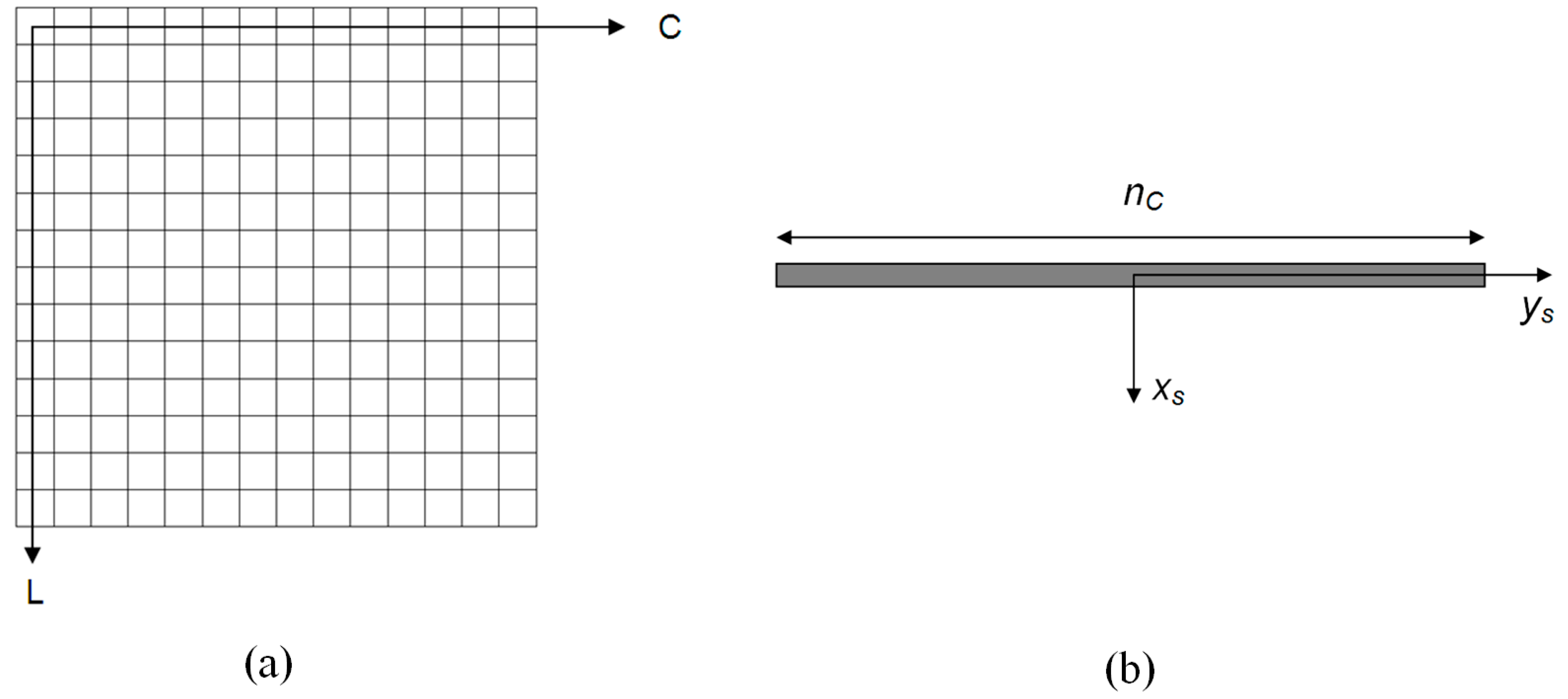
The first reference system related to images is the Image Reference System (IRS). This system is associated with the two-dimensional array of image pixels in a column (
C) and line (
L) coordinate system. The system’s origin is at the centre of the top left image pixel, as shown in
Figure 1a. Another system related to the linear array CCD chip is the Scanline Reference System (SRS), which is a two-dimensional system of coordinates. The origin of the system is located at the geometric centre of the linear array CCD chip. The
xs axis is parallel to the
L axis and is closest to the flight direction. The
ys axis is perpendicular to the
xs axis, as shown in
Figure 1b.
The mathematical transformation between IRS coordinates and SRS coordinates is presented in Equations (1) and (2).
where
PS is the pixel size of the CCD chip in mm and
nC is the number of columns of the image.
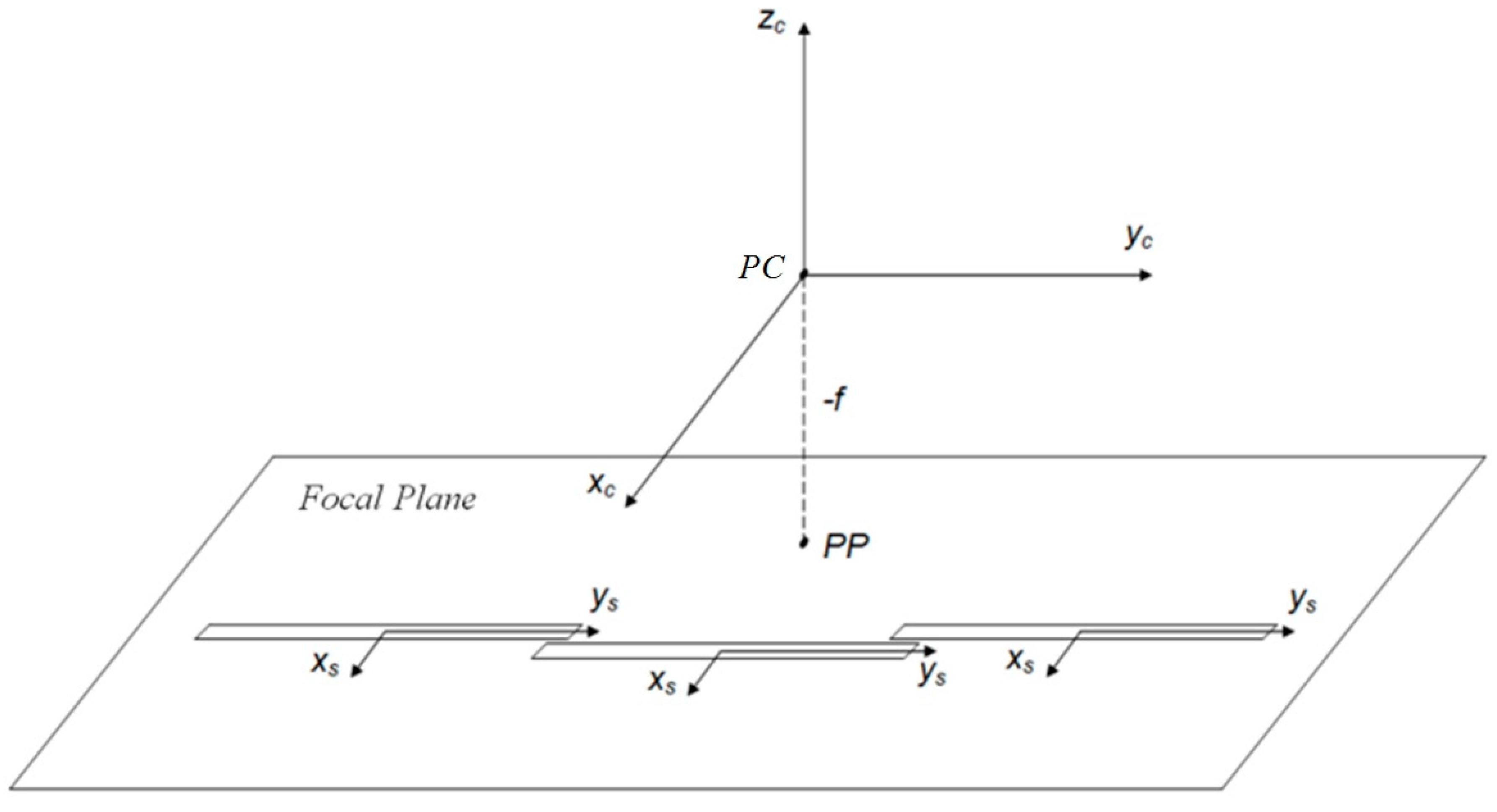
The Camera Reference System (CRS) is a three-dimensional system. Its origin is at the perspective centre (PC) of each camera lens. The
xc and
yc axes are parallel to the
xs and
ys axes. The
zc axis points upward and completes a right-hand coordinate system [
11]. The projection of the PC in the focal plane defines the principal point (PP), and the focal length
f is the distance between the PC and PP. An illustration of the CRS and SRS in a focal plane with three CCD chips is shown in
Figure 2.
The transformation between SRS coordinates and CRS coordinates is presented in Equation (3).
where
dx and
dy are translations from the centre of a CCD chip to the PP in the focal plane.
3. PRISM Sensor
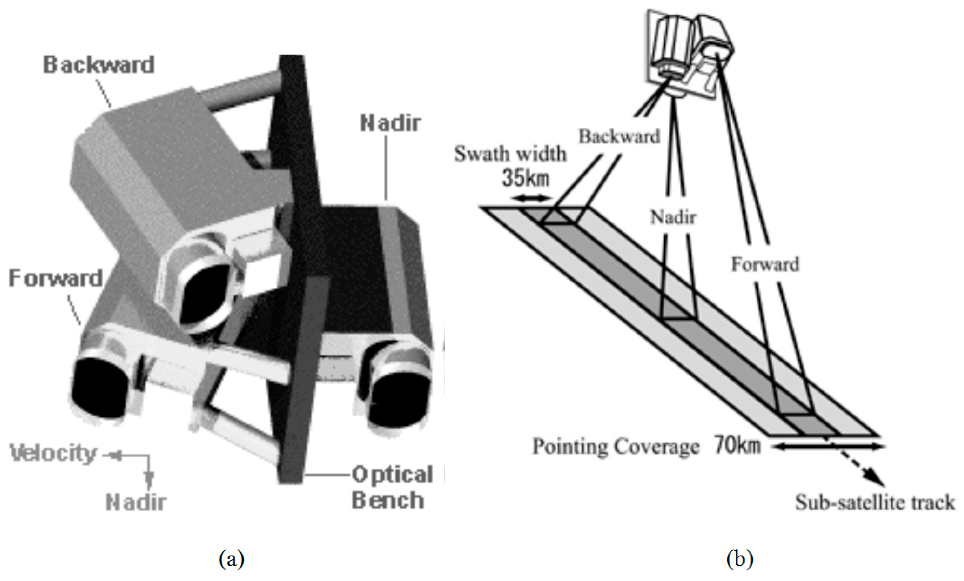
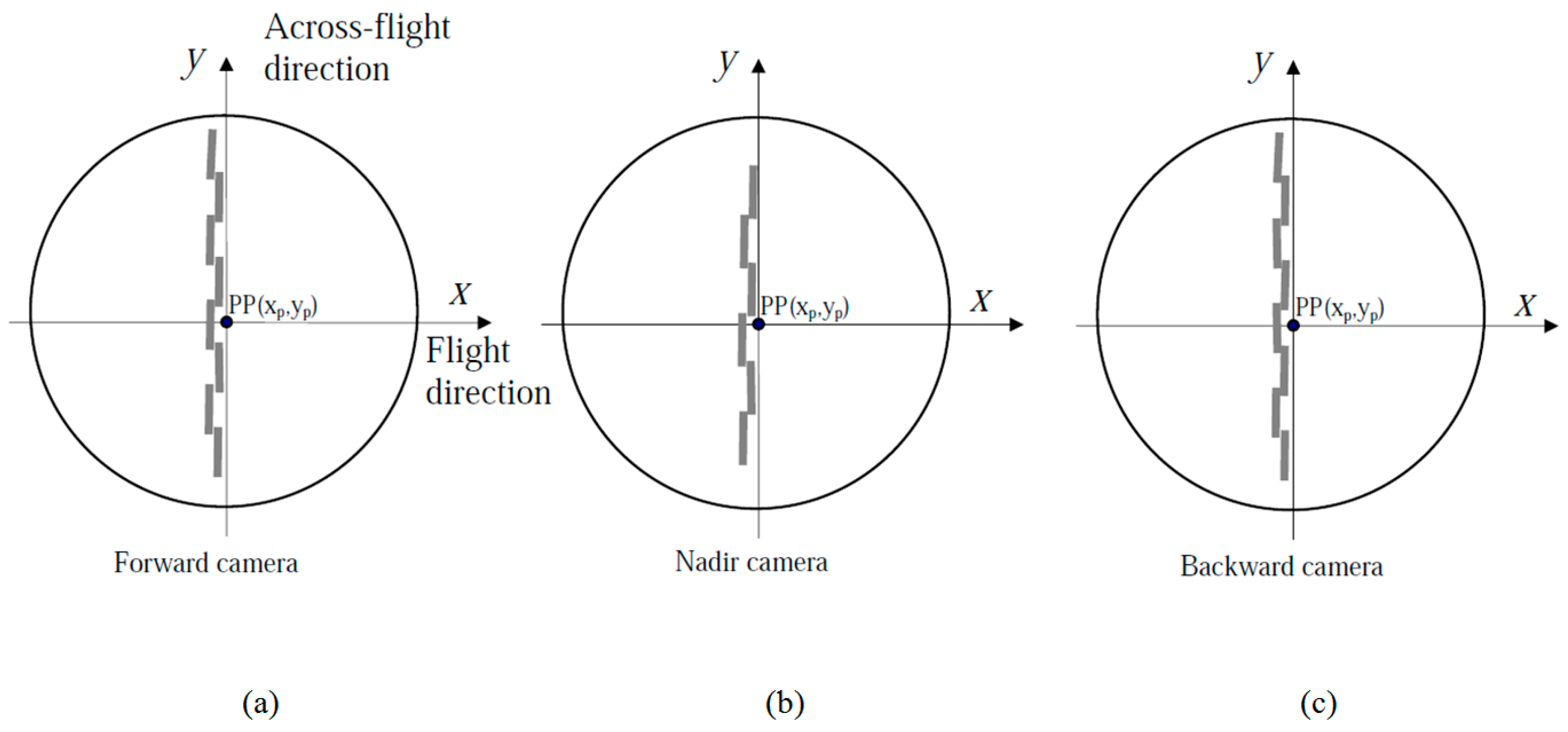
The PRISM sensor provides images with a ground sample distance (GSD) of 2.5 m, and a radiometric depth of 8 bits in a spectral range from 0.52 to 0.77 μm. The sensor is composed of three independent cameras in the forward, nadir and backward along-track directions, as shown in
Figure 3a. The simultaneous imaging by the three cameras is called the triplet mode and covers a range of 35 × 35 km on the ground, as shown in
Figure 3b. The forward and backward viewings were oriented to ±23.8 degrees with respect to nadir viewing to obtain a base/height ratio equal to one [
1].
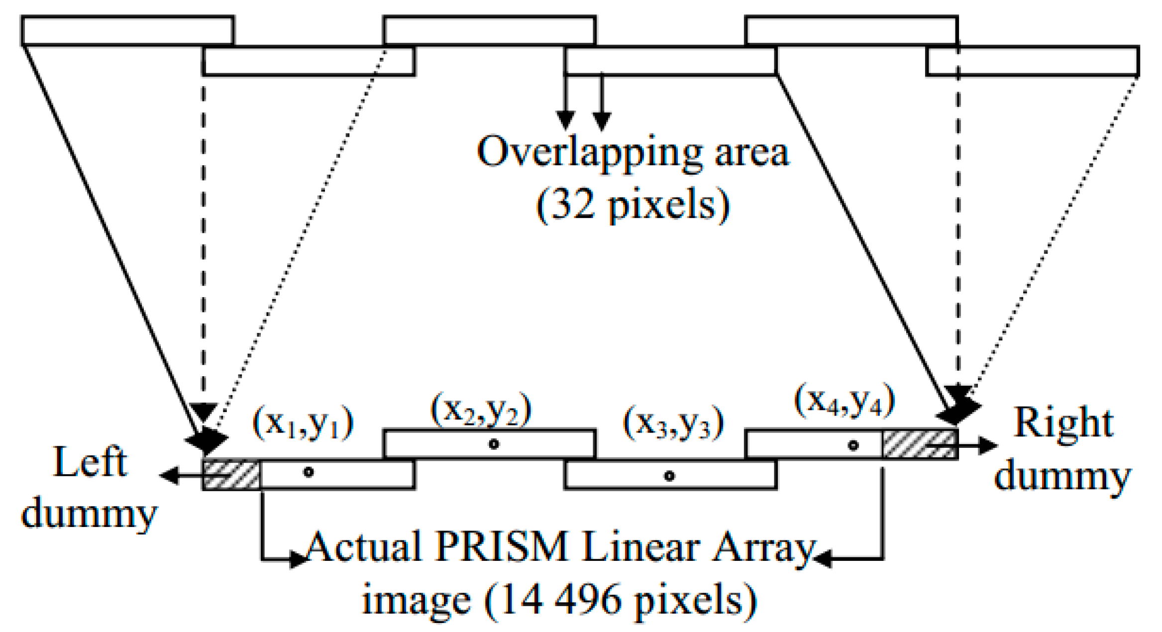
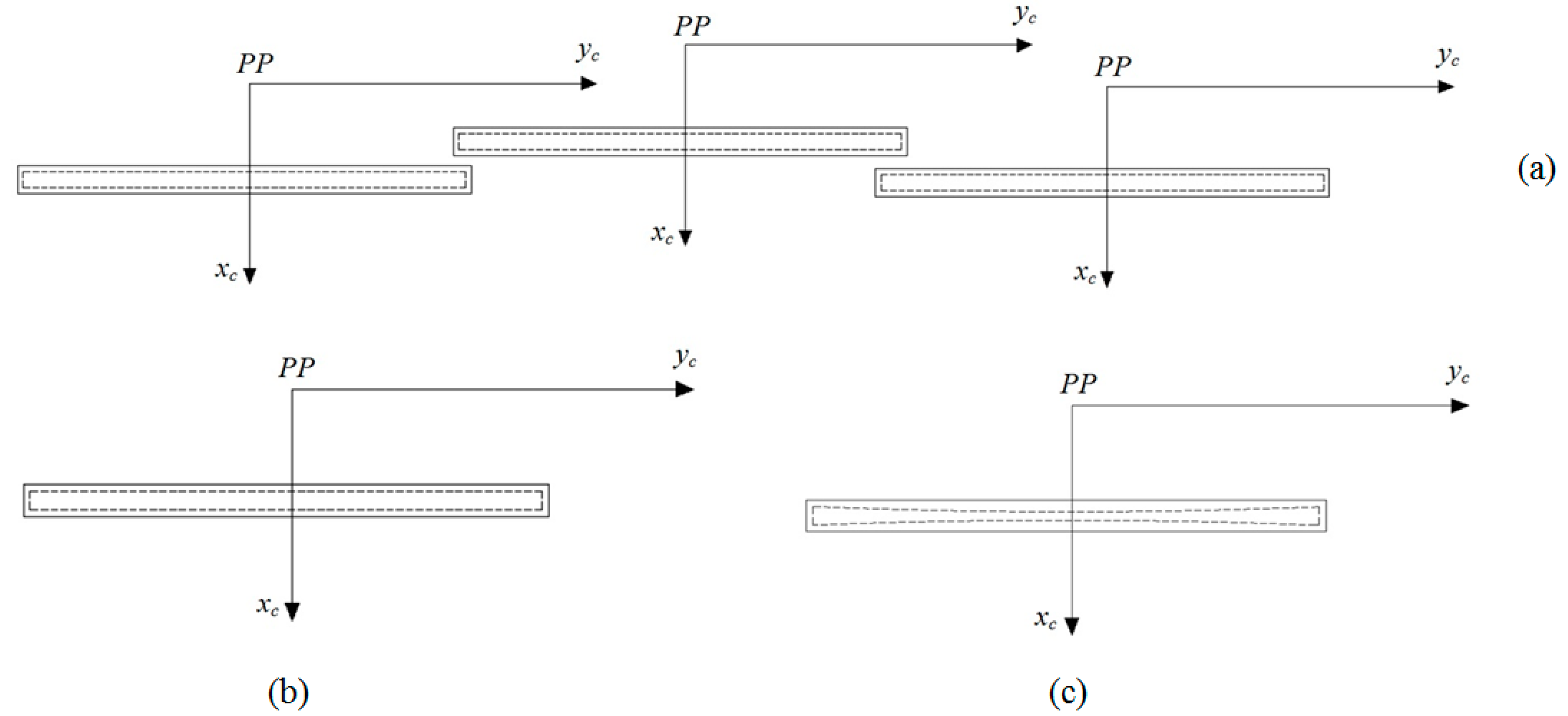
In the focal plane of the backward and forward cameras, eight CCD chips, each with 4928 columns, were placed. In the focal plane of the nadir camera, six CCD chips, each with 4992 columns, were placed. The CCD chips overlap by 32 columns. In
Figure 4, the arrangement of the CCD chips in the focal planes of the forward, nadir and backward cameras are presented.
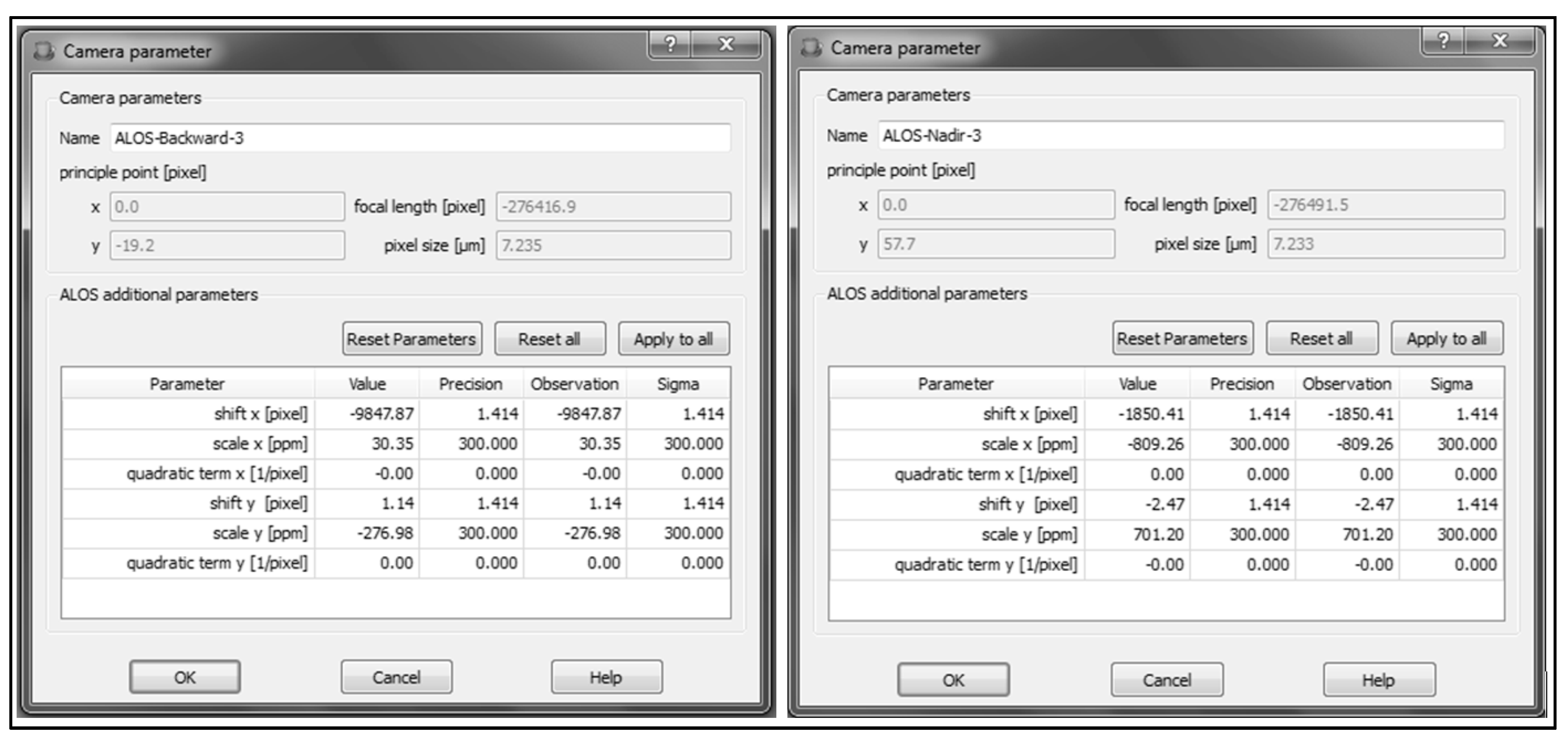
For the arrangement of the final image distributed to users, with 14,496 columns and 16,000 lines, a set of four CCD chips was selected. Further pixels were not used at the left and right sides. In
Figure 5, an example of the nadir image is shown. An on-orbit geometric calibration, performed by JAXA in June 2007, computed the following parameters: translation values of each CCD chip centre with respect to PP, the focal lengths, the sizes of pixels in the CCD chips, and the PP coordinates
x0 and
y0. These parameters were provided to some researchers, as can be seen in [
6,
7]. This dataset is currently embedded in BARISTA software, developed by project 2.1 of the Cooperative Research Centre for Spatial Information [
7]. The calibrated values of the focal lengths of the backward, nadir and forward cameras are shown in
Table 1.
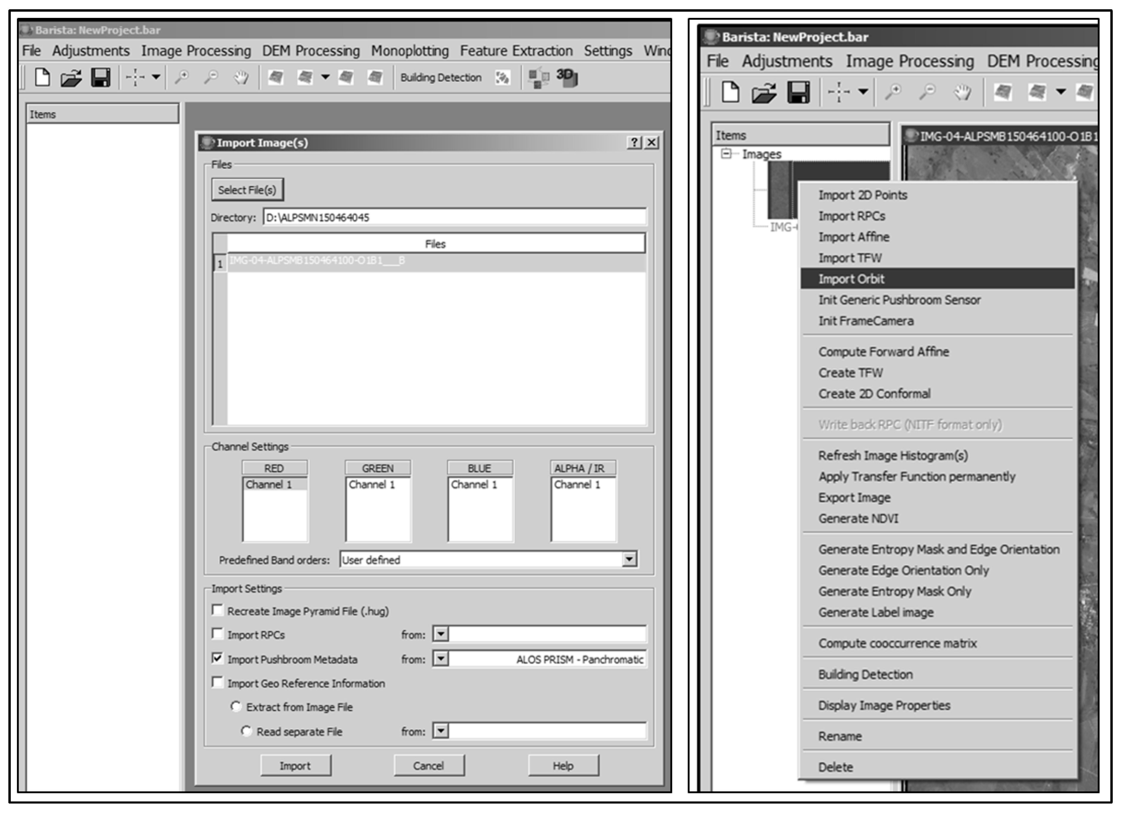
An example of the input step of the PRISM sub-image files and extraction of the mentioned data set are shown in
Figure 6 and
Figure 7, respectively.
ALOS PRISM images are made available to users at four different processing levels. The processing levels and characteristics of each level are shown in
Table 2 [
1]. For the application of rigorous models, processing levels 1A or 1B1 must be used.
4. Mathematical Modelling
The accuracy of orientation using the rigorous model is directly related to the accuracy of the interior orientation. The IOP can be estimated by calibration in the laboratory before the satellite launches. However, the physical conditions in this case are not the same as those found when the satellites are in orbit. According to [
2], during the launch of a satellite, the environmental conditions change rapidly and drastically, causing changes to the internal sensor geometry. According to the authors, the environmental conditions after orbit stabilization are also harsh, and may cause internal geometry changes; however, this is not as crucial as the changes that occur during launch. According to [
3], the large acceleration during a launch may change the exact position of the CCD-lines in the camera and the relation between the CCD-lines. Consequently, at least their geometric linearity must be verified after launch. In addition, according to the same author, the systematic lens distortion can be calibrated before launch but may be influenced by the launch. Furthermore, the thermal influence of the sun can cause changes in the internal sensor geometry. Consequently, to exploit the full geometric potential of a sensor, the IOP should be re-estimated after a satellite launches, preferably periodically. For the PRISM ALOS cameras, JAXA conducted a re-estimation of the parameters multiple times after launch, such as the June 2007 calibration mentioned above.
Considering the IOP of an orbital CCD linear array sensor in addition to the focal length (
f) and sizes of the pixels in the CCD chip (
PS), Poli [
13] proposed two parameter sets. The first set of parameters is the IOP related to the optical system. These parameters are the PP coordinates
x0 and
y0, the change in the focal length Δ
f, the coefficients
K1 and
K2 of the symmetric radial lens distortion, and the scale variations
sx and
sy in the
xs and
ys directions, respectively. The scale variation effect is only considered in the
ys direction when the CCD array is equal to a linear array. Examples of the effects of IOP related to the optical system are shown in
Figure 8.
The correctives terms
dxf and
dyf for the effects of change in the focal length in the
xs and
ys directions and symmetric radial distortion terms
dxr and
dyr are given by:
with:
The correction to the scale variation in the
ys direction is:
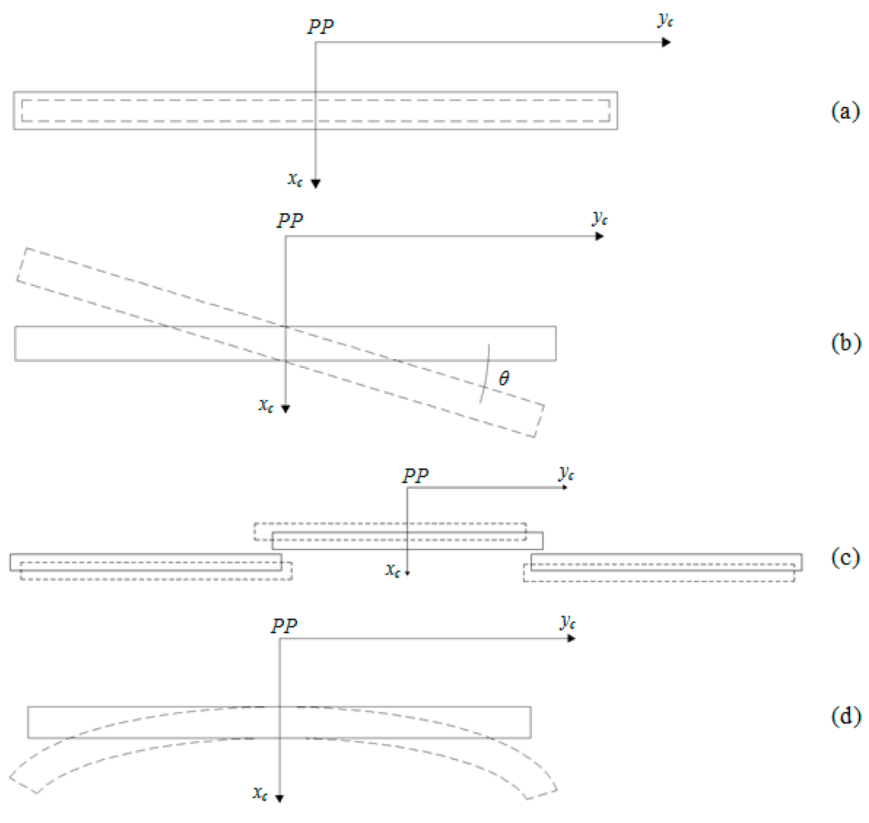
The second set of IOP is related to the CCD chip. These parameters are the change of pixel dimensions in the
xs and
ys directions,
dpx and
dpy; the two-dimensional shift
a0 and
b0; the rotation θ of the CCD chip in the focal plane with respect to its nominal position; and the central angle of the effect of a line bending in the focal plane, considering that the straight CCD line is deformed into an arc. As in the case of the scale variation effect, for a linear array sensor, the parameter
dpx can be disregarded. As seen in [
6], the CCD chip displacements
dx and
dy, with respect to the PP, can also be considered IOP related to the CCD chip. Examples of effects of the IOP related to the CCD chips are shown in
Figure 9.
The two-dimensional shift parameters
a0,
b0 are added to the
dx and
dy quantities.
The effect of the change of pixel dimension in the
ys direction (
dpy), CCD chip rotation in the
xs and
ys directions (
dxθ,
dyθ) and line bending in the
xs (
dxδ) direction are given by:
where
In this research, all of the mentioned IOP were initially considered, except the
dpy parameter, because its effect is similar to the effect caused by the scale variation in the
ys direction (
Figure 8 and
Figure 9). The
sy parameters were considered different for each CCD chip to get closer to the physical reality and avoid strong correlations with the change in the focal length, unlike that considered in [
6]. The central angle δ of the bending effect was also considered unique for each CCD chip.
Since the corrective terms
dyθ and
dys of rotation and scale variation in the
ys direction are functions of their own coordinate
ys, they were grouped into a single correction term (
a1 and
b1):
where
The term of rotations in the
xs direction was considered:
The IOP
dx,
dy,
x0 and
y0 were fixed with their nominal values since the residual errors are absorbed by the parameters
a0 and
b0. The nominal values of the focal lengths used in BARISTA software were also fixed since their uncertainties were estimated from the Δ
f parameters. The IOP
a0,
b0 and
a1,
b1 were estimated using weighted constrains with a standard error of 1.5 pixels and 300 ppm, respectively, and the latter was as adopted in BARISTA software [
7]. To define the reference system and avoid singularities, as adopted in [
7], for each of the three PRISM cameras, one CCD was selected as the master chip. In this research, the second CCD chip was considered the master CCD chip. As a result, the parameters
a0,
b0 and
a1,
b1 for this CCD chip were fixed, and its systematic errors were absorbed by the EOP. The mathematical transformation of SRS coordinates to CRS coordinates, considering the set of IOP, is given by the following equations:
The collinearity equations with the IOP are:
with:
where
X,
Y,
Z and
XS (
t),
YS (
t),
ZS (
t) are, respectively, the object space coordinates of a point and the PC sensor at an instant
t; and
r11 (
t), ...,
r33 (
t) are the elements of the rotation matrix
R (
t), which is responsible for aligning the CRS with the TRS at a given instant
t. Since the satellite attitude data were not available for the images used in this research, the rigorous model considered in this study was a Position-Rotation type, as described in [
14]. Thus, the rotation matrix
R (
t) was defined as a function of the nonphysical attitude angles
ω,
φ, and
κ, which vary in time:
After considering all of the mentioned IOP, significance and correlation analyses were performed between the parameters to find an optimal group of IOPs that could be used. The IOP significance test was based on a comparison of the estimated parameter value with its standard deviation, obtained from the variance-covariance matrix. When the IOP value was lower than the value of its standard deviation, it was considered non-significant and, consequently, was without importance in the final mathematical model. This test was performed iteratively, analysing one IOP at a time. The correlation analysis between IOP aimed to identify dependencies and the loss of physical meaning in the value of the parameter. In this research, the correlation was considered strong when the value of the correlation coefficient was higher than 0.75 or 75%.
5. Platform Model
Based on the second-order polynomial platform model, Michalis [
11] indicated that the first-order coefficient represents the velocity of the satellite on the reference axis and, similarly, the second-order coefficient represents the acceleration on the same axis. This platform model is called the UCL (University College of London) Kepler model. The components of the acceleration are calculated from the components of the position, using the mathematical formulation of the two-body problem [
15]. The components of the sensor PC position on the satellite are calculated using the theory of Uniformly Accelerated Motion, as shown in Equations (28)–(30).
where
X0,
Y0,
Z0 and
ux,
uy,
uz are, respectively, the position and velocity components of the sensor PC at the time at which the first line of the image was obtained;
t is the acquisition time of an image line; and
GM is the standard gravitational parameter.
The rotation angles of the sensor may be considered constant during the image acquisition time [
16] or can be propagated by polynomials [
8,
9,
10,
12], depending on the satellite’s motion characteristics. In this research, the rotation angles
ω and
φ were considered invariant since the image acquisition occurred in approximately 6 s and the attitude control of the ALOS has sufficient accuracy [
17]. However, the
κ angle was considered variable, being modelled by a second-order polynomial, as shown in Equations (31)–(33). This is due to the yaw angle steering operation, which is intended to continuously modify and correct the satellite yaw attitude according to the orbit latitude argument to compensate for the effects of the Earth’s rotation on the sensor image data [
17] (crab movement).
where
ω0,
φ0, and
κ0 are the orientation angles in the first line of each image; and
d1,
d2 are the polynomial coefficients of
κ0 variation.
An important issue in the use of this platform model is that the coordinates in the object space of control, or check points, must be referenced to the GCRS due to the mathematical formulation of the two-body problem in the calculation of acceleration. Normally, the coordinates of the points collected in the object space are referred to a TRS. To avoid the transformation of coordinates from TRS to GCRS, the platform model composed of Equations (28)–(30) was adapted. In this transformation, the movements of precession and nutation, and polar motion must be taken into consideration in addition to the Earth’s rotation [
15].
However, according to [
18], in a short period of orbit propagation, the effects of precession and nutation and polar motion can be disregarded. Once the PRISM images with 16,000 lines are formed in approximately 6 s, only the influence of the Earth’s rotational movement was added to the equations of the two-body problem. Thus, the UCL platform model adapted for the use of coordinates referenced to a TRS is defined as follows:
with:
where
ωt is the magnitude of the Earth’s rotational angular velocity.
The advantage of using the UCL Kepler model instead of models that use polynomials is the reduction in the number of EOP unknowns in each image triplet. For the ALOS satellite, the components of position and velocity from GPS
XGPS,
YGPS,
ZGPS,
uxGPS,
uyGPS, and
uzGPS are available in the .SUP files, ancillary 8, with a sampling interval of 60 s for the day on which the image was obtained [
1]. The data are provided by the GPS receiver that is on board the satellite. To estimate the state vectors referring to the instant of acquisition of the first lines of each image, a spline interpolation was used. In this process, the minimum accuracy of the spline interpolation, omitting a central point and using 34 surrounding points, was 6 mm for positions and 7 µm/s for velocities. These interpolation results are in agreement with those obtained by [
19,
20], who used the Hermite interpolator. However, the components of the position and velocity from GPS have uncertainties
XT,
YT,
ZT,
uxT,
uyT, and
uzT when accurate orbit determination is not applied by JAXA. Thus, the components
X0,
Y0,
Z0,
ux,
uy and
uz were obtained by:
The values of XGPS, YGPS, ZGPS, uxGPS, uyGPS, and uzGPS are fixed in the estimation process by least squares adjustment. To avoid strong correlations with the parameters related to the systematic changes of CCD chips positions in the focal planes, the parameters XT, YT, ZT, uxT, uyT, and uzT received weighted constraints in the least squares adjustment. As mentioned above, the satellite attitude data were not available for the images used in this research. Therefore, the EOP ω0, φ0, κ0, d1 and d2 did not receive weighted constraints. To identify the strong dependencies between EOP and IOP and avoid inaccurate results or the loss of the physical meaning of parameters, correlation analyses were performed using values obtained from the covariance matrix. Similarly, the correlation was considered strong when the value of the correlation coefficient was higher than 0.75 or 75%.
Since the state vectors are referenced to ITRF97, the value of ωt was 7,292,115 × 10−11 rad/s. The value of the GM used was the one indicated in the SUP file, which was 3.986004415000000 × 10¹⁴ m3 s−2.
6. Test Field and Experiments
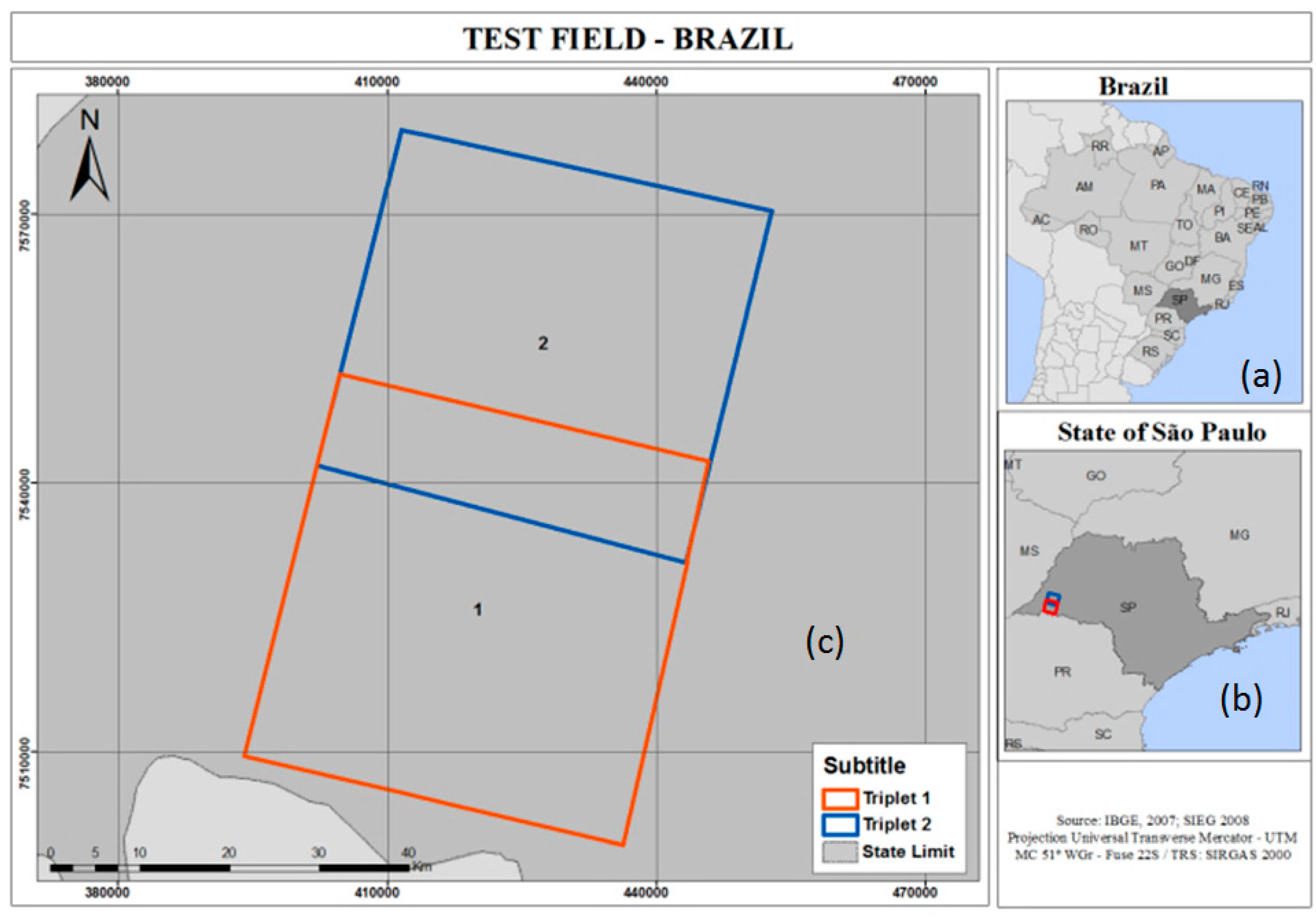
In this research, were used two neighbouring PRISM triplets, at processing level 1B1, obtained on the same path, both in 20 November 2008. The test field covered by the images included the city of Presidente Prudente and adjacent regions in the state of São Paulo, Brazil.
Figure 10a shows the location and the areas covered by the triplets used in this study, which were called triplets n.1 and n.2. In
Figure 10b,c, the location of triplets within the state of São Paulo and the location of the state of São Paulo in Brazil are shown, respectively.
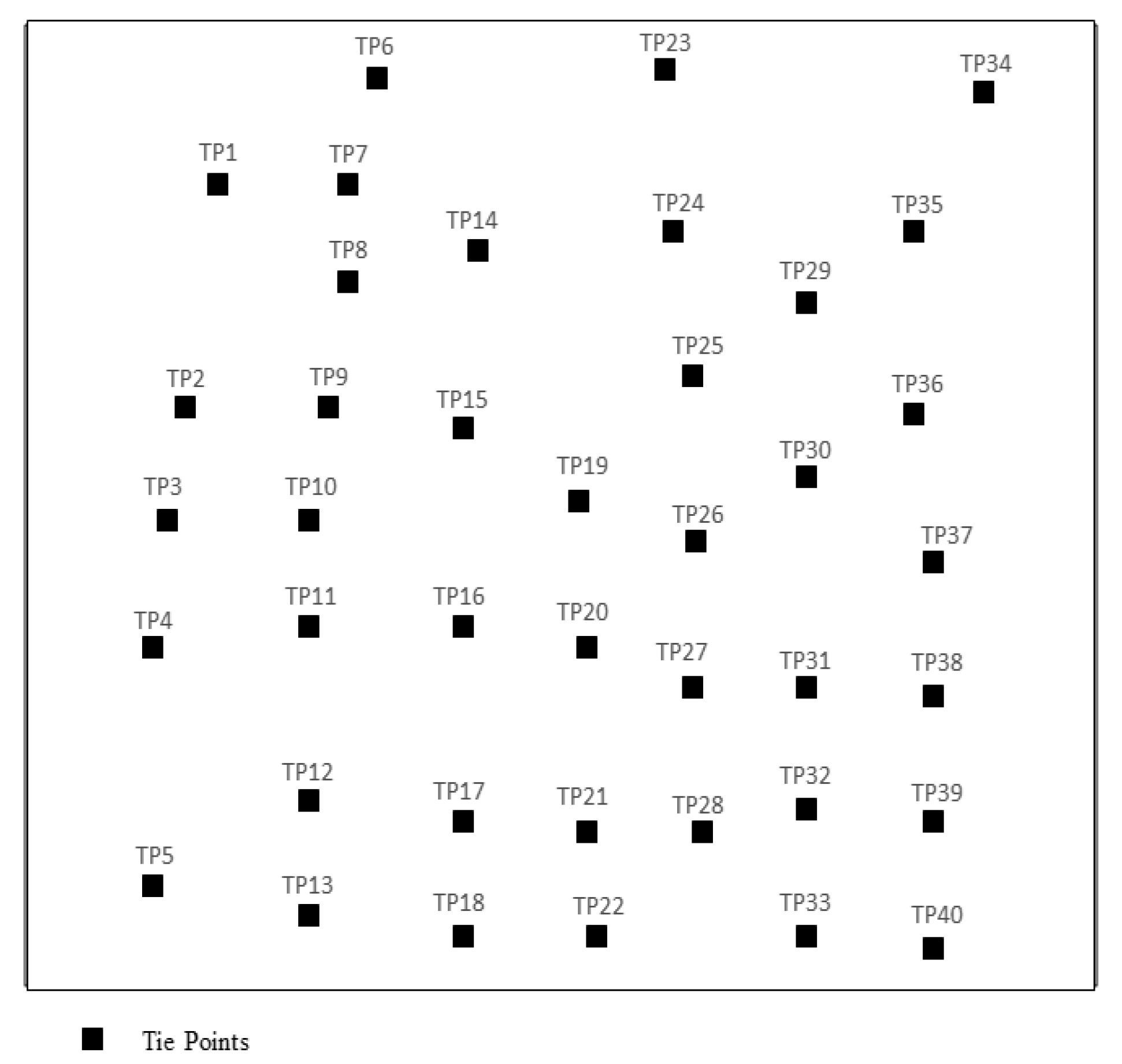
In each triplet, forty tie points were collected and distributed homogeneously. An example is shown in
Figure 11, with the distribution of these points in triplet n.1. All points were manually collected in the three images of each triplet; i.e., all points have three image measurements.
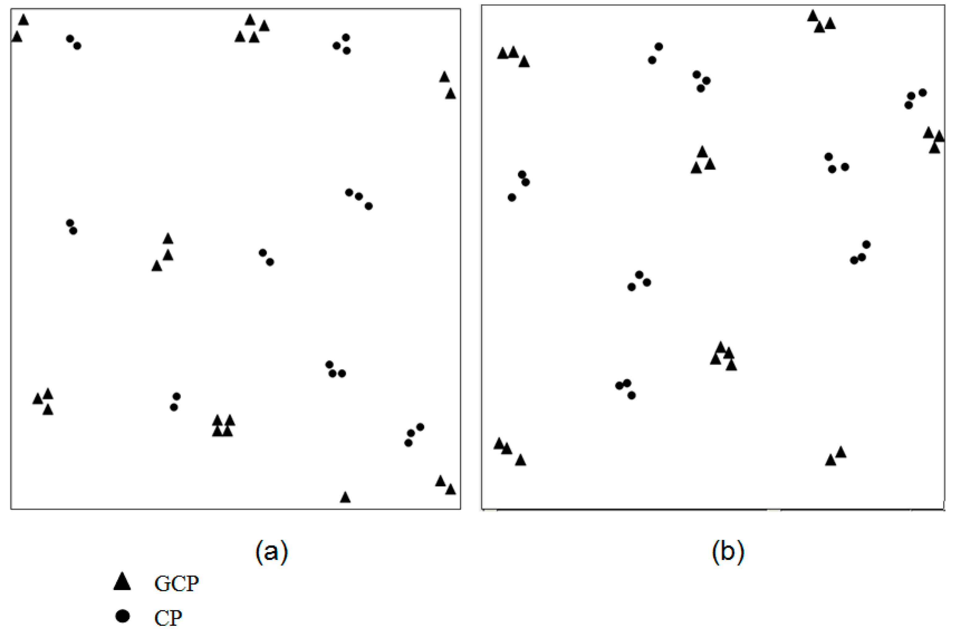
The coordinates of the ground control and check points were extracted from orthophotos with 1 m GSD and from Digital Terrain Models (DTM) with 5 m GSD generated from aerial images. The positional accuracy of the orthophotos and the altimetric information extracted from the DTM are, respectively, compatible with the 1:2000 and 1:5000 scales, and class A of the Brazilian Planimetric Cartographic Accuracy Standard. This means that 90% of the points present errors less than 1 m and 2.5 m. In the area covered by triplet n.1, 22 ground control points and 20 check points were collected. In the area covered by triplet n.2, 21 ground control points and 24 check points were collected. In
Figure 12a,b, the distributions of the control and check points in the area covered by triplets n.1 and n.2 are shown, respectively.
In
Table 3, the numbers of ground control points and check points on each CCD chip for the three cameras of triplets n.1 and n.2. are shown.
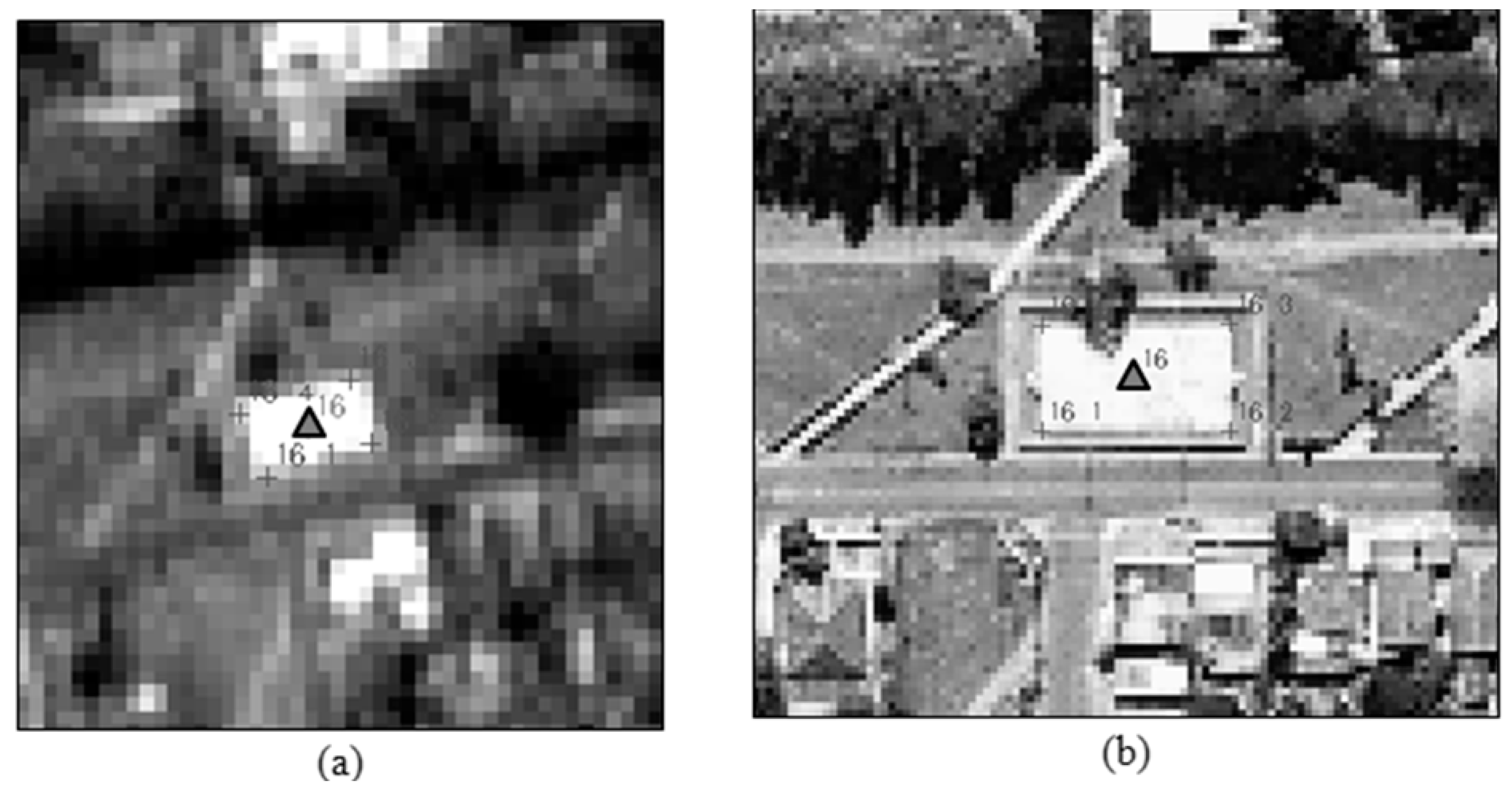
To facilitate the measurement of ground control and check points on the images and orthophotos, the determination of centroids of geometric entities was utilized, as presented in [
21]. The geometric entities used were buildings, soccer fields, courts, or anthropic structures of other types. As an example, in
Figure 13a, the coordinates of point 16 in the space image, that is, in the PRISM images, were obtained from the coordinates of points 16_1, 16_2, 16_3 and 16_4. In
Figure 13b, point 16 obtained in the object space, that is, in the orthophotos, in the same way is shown. After estimating the planimetric coordinates of the centroids points, the altimetric coordinates were extracted from the DTM of the region.
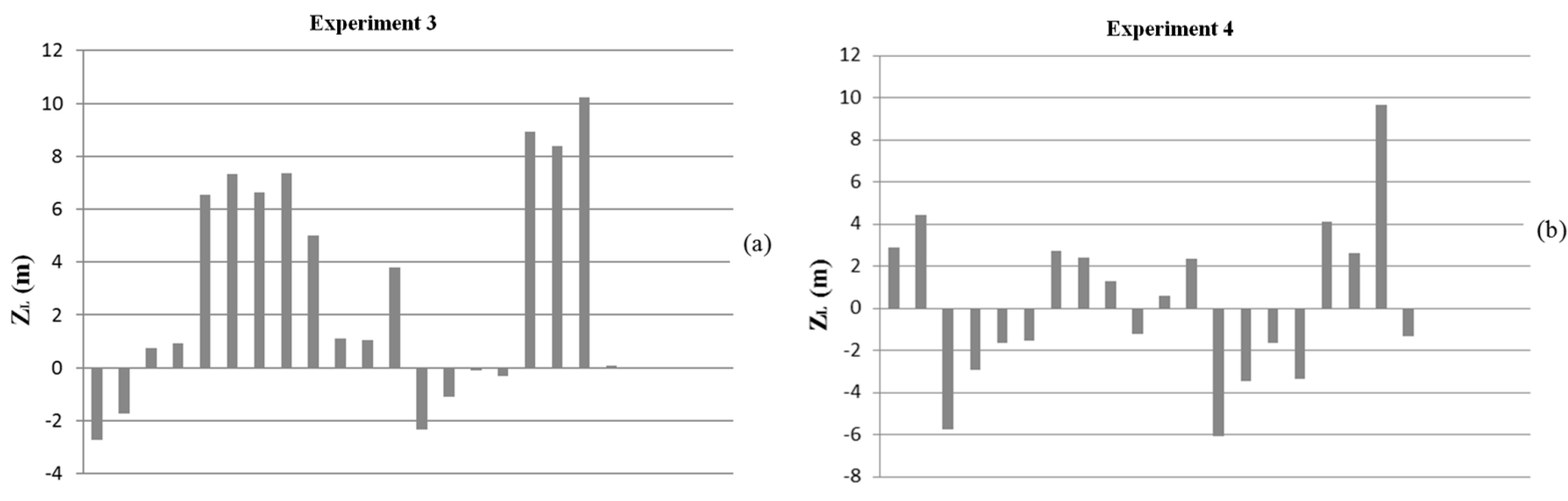
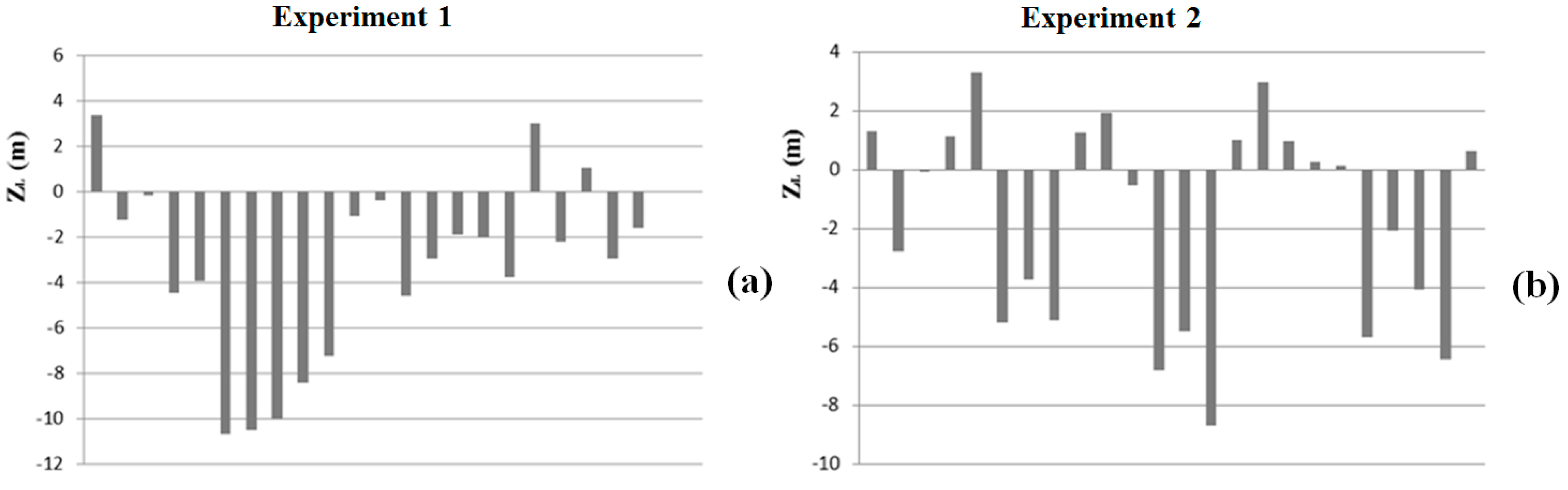
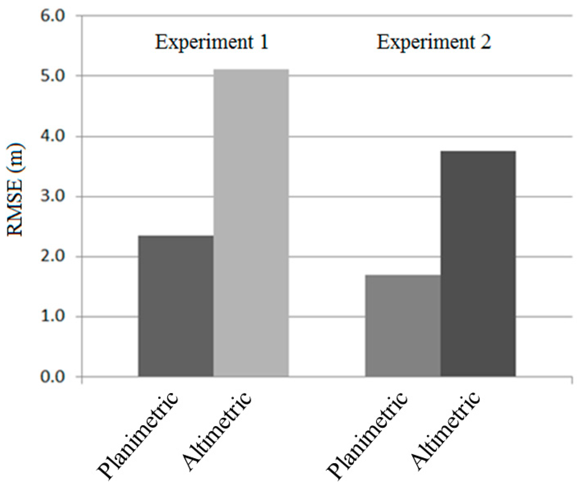
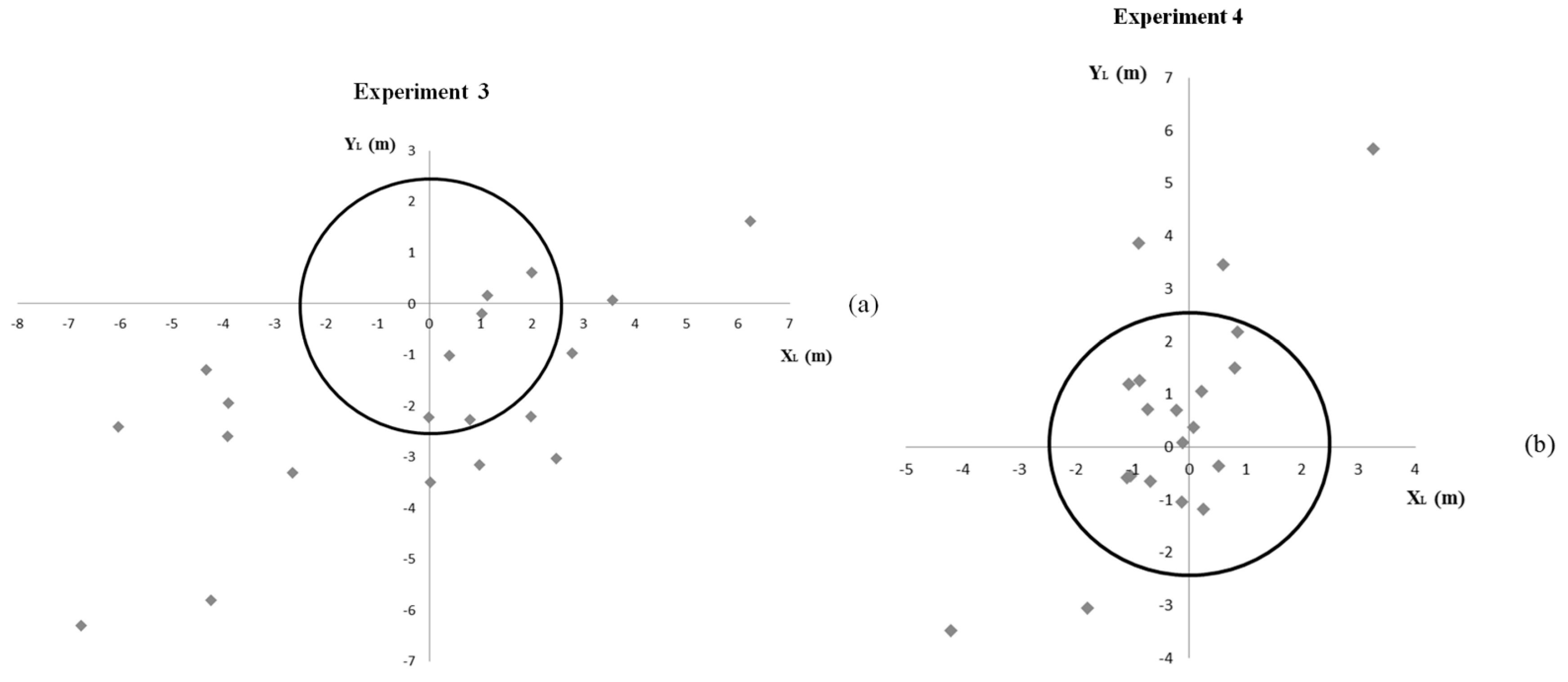
In this research, four experiments were carried out using triplets n.1 and n.2. In experiments 1 and 2, the bundle adjustment trials of triplet n.1 with and without the estimation of IOP were performed. To analyse the quality of the obtained IOP from experiment 2, in experiment 4 they were used to perform the bundle adjustment of triplet n.2. In experiment 3, the bundle adjustment of triplet n.2 was performed without the use of the IOP estimated in experiment 2. The results obtained from experiments 3 and 4 are compared and discussed in the next section. In
Table 4, the configuration of each experiment is shown.
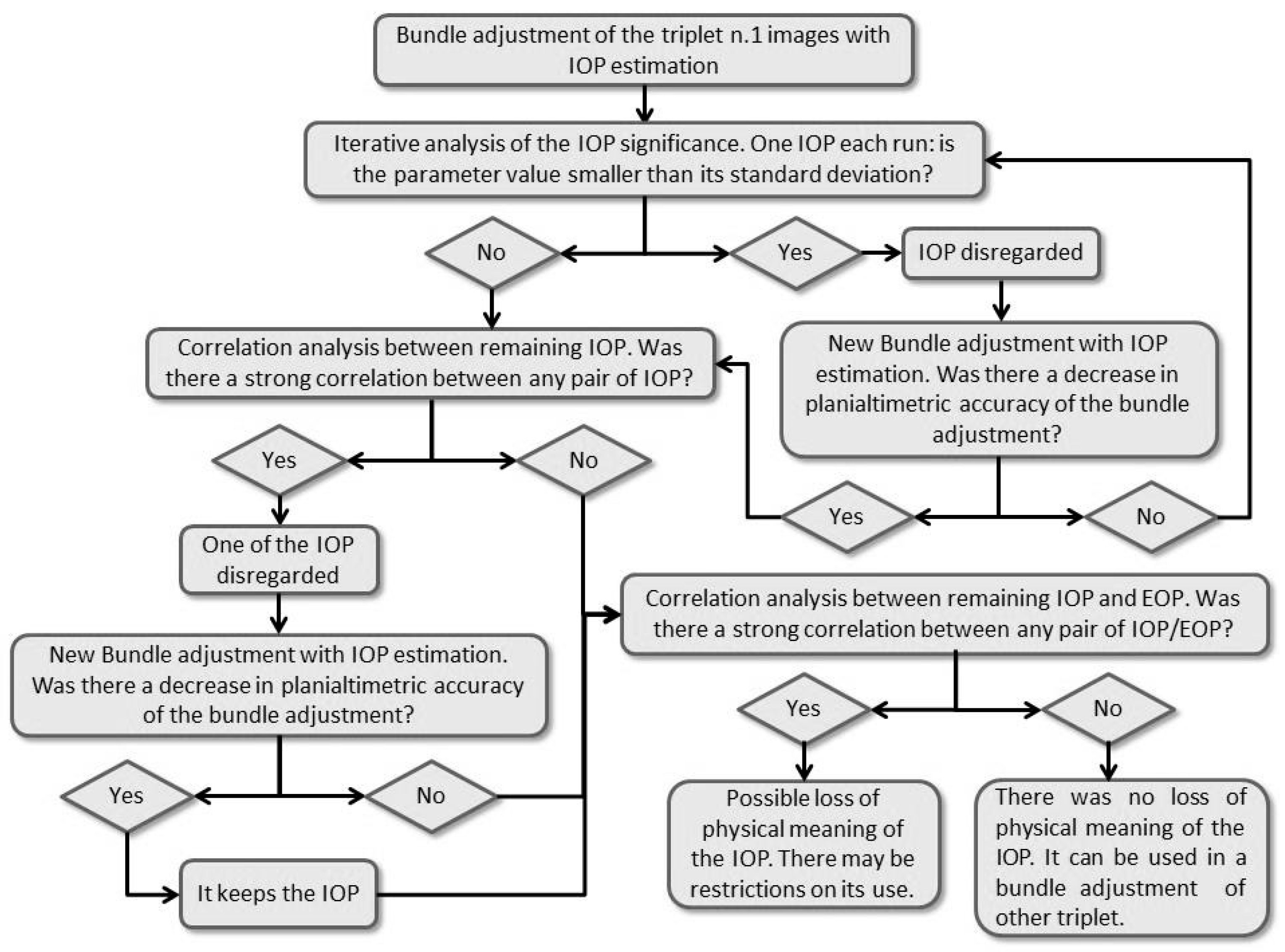
In experiment 2, in addition to the IOP correlation analysis, the correlations between IOP and EOP were estimated. The procedures for the analyses were previously mentioned in
Section 4 and
Section 5. To better demonstrate the steps of the proposed methodology in experiment 2, a workflow is shown in
Figure 14.
8. Discussion
In light of the results obtained in the experiments, a synthesis can be given. Regarding the accuracy, in the bundle adjustment with IOP estimation, improvements were observed in comparison to the bundle adjustment without IOP estimation, mainly in the altimetric component. While the resulting planimetric accuracy improved by 0.65 m, the altimetric accuracy improved by 1.36 m. However, it is important to highlight that the measurements in the image space of the control and check points used in the bundle adjustment were refined by using the centroids methodology, presenting a quality better than 1 pixel. It is also worth mentioning that the magnitudes of the planimetric accuracies found in this research are close to those found in [
6,
7], which used different platform models and different IOP sets from those used here. In contrast, the magnitudes of the altimetric RMSE values found in this research were larger, that is, less accurate than those found in the cited studies.
Two questions that were not addressed in the works carried out by [
6,
7] are the analysis of significance of IOP and the correlation between them. This is done with the objective of analysing the importance of the parameter, with a possible loss of physical meaning and a possible simplification of the functional mathematical model. In the significance analysis, it was observed that the effects of the symmetrical radial distortions of the lens systems, of the rotations of the CCD chips in the focal plane and of the scale variation in the
ys direction were not significant. Consequently, these parameters could be ignored. For the effect of bending of the CCD chip, the parameter was only significant in chip 2 of the nadir camera. The effect of systematic change in focal length was significant in all cameras. The parameters related to systematic changes CCD chip positions in the focal planes did not present a homogeneous behaviour. After analysing the correlation between the significant IOP, it was verified that only the IOP
δ_
chip2 could be ignored without a significant change in planialtimetric and altimetric accuracies.
An issue that was not analysed in [
6,
7] was the application of the IOP estimated with one triplet in the bundle adjustment of a different triplet. After the correlation analyses between the IOP and EOP, strong correlations were detected between the IOP
a0_chip1 and
a0_chip4 of the backward camera and the EOP
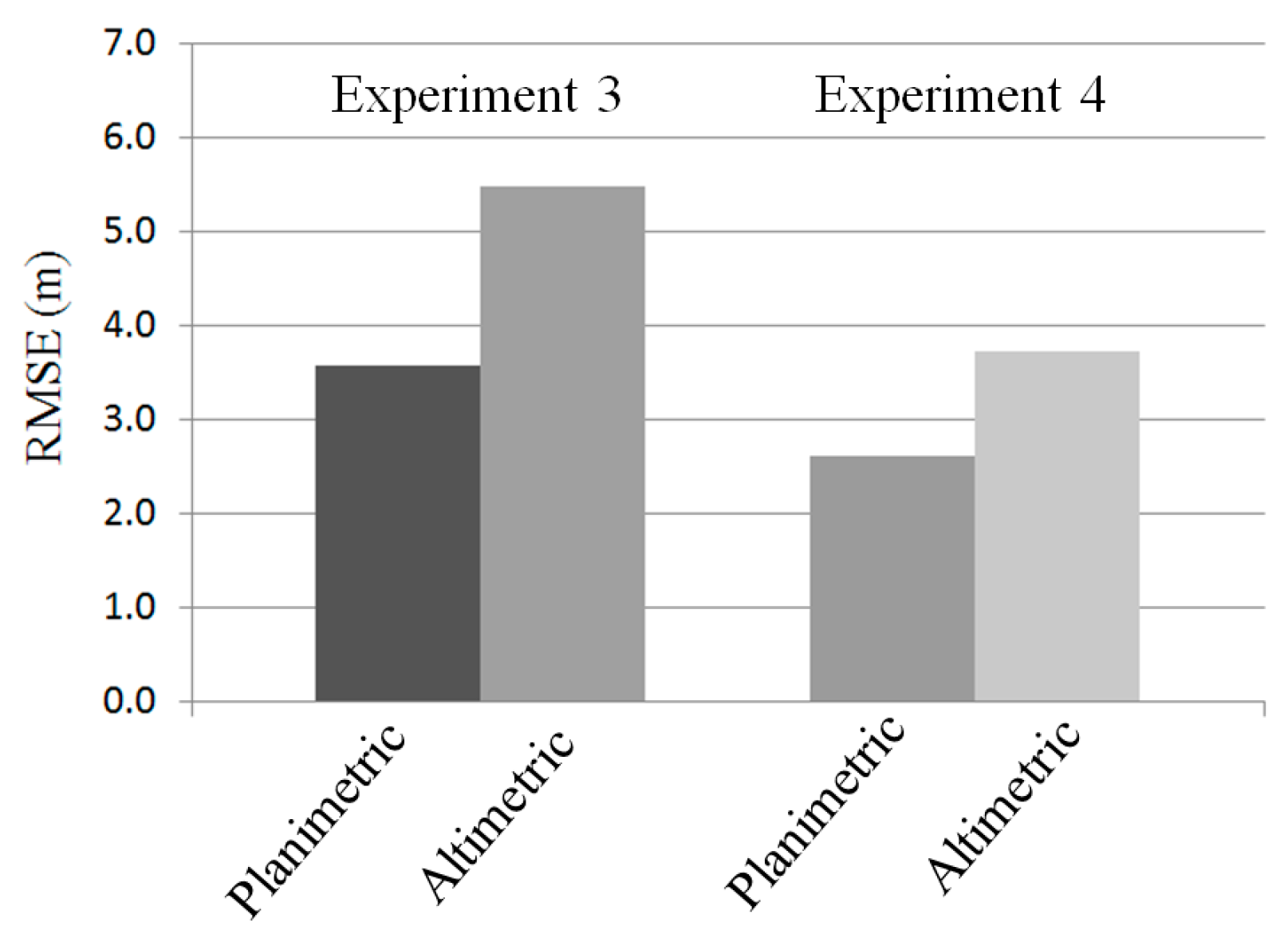
κ0, indicating a possible loss of physical significance of the IOP. Even so, when IOP were applied to the bundle adjustment of triplet n.2, there were planimetric and altimetric improvements compared to bundle adjustment without the use of IOP.
It should be noted that even though this satellite is out of operation, the images obtained by it remain in archives and are still being used in several applications. In addition, the methodologies investigated in this article can be applied to other linear array pushbroom sensors with similar characteristics. As an example, we can cite the images obtained by the ZY-3 Chinese satellite.
9. Conclusions and Recommendations
This study investigated the importance of estimating IOP to compute 3D coordinates by photogrammetric intersection with bundle adjustment using a PRISM image triplet. Additionally, the study proposed some improvements in the platform model developed by Michalis [
9] to use coordinates referenced to the TRS ITRF97. The bundle adjustment with IOP estimation improved the quality of 3D photogrammetric intersection. Considering the RMSE of the 3D discrepancies in check points, the planimetric and altimetric accuracies increased 0.65 and 1.36 m, respectively. After the bundle adjustment with IOP estimation, a trend in the southern area of the experimental set was observed. However, the sample of discrepancies in Y component was considered normal by the Shapiro-Wilk test considering the expected planimetric accuracy of one GSD.
Ground control points’ and check points’ coordinates were obtained from the determination of centroids points of geometric entities, such as buildings, soccer fields and courts. This procedure provides an improvement in the precision of measurements of points, both in the image space and the object space. This can be confirmed since, in all experiments, more than 97% of the residual values of the observations after bundle adjustment were lower than 1 pixel.
In the bundle adjustment with IOP estimation, only part of the IOP related to systematic changes in CCD chip positions in the focal planes and the IOP related to changes in focal lengths was considered significant. The effects of the rotation and bending of CCD chips, the symmetric radial distortion of the lens and the scale variation in the ys direction could be discarded without affecting the accuracy results.
The practical analysis of the usability of the estimated IOP from an independent triplet to be used in other applications was performed. The IOP estimated from triplet n.1 were applied to the bundle adjustment of triplet n.2. Despite the strong correlations between the IOP a0_chip1 and a0_chip4, and the EOP κ0 in the backward camera, the result of using these IOP was satisfactory. The improvements in the planimetric and altimetric accuracies were 0.40 m and 1.75 m, respectively.
For future studies to be developed, it is recommended to verify the estimation of the IOP of the PRISM sensor by using the polynomial model presented in [
7] in conjunction with the adapted UCL platform model; to estimate the IOP of other sensors using the methodology used in this study; and to analyse the use of collinearity and coplanarity rigorous model with ground control points and straight lines.


