Article

The 2013 FLEX—US Airborne Campaign at the Parker Tract Loblolly Pine Plantation in North Carolina, USA

1
Biospheric Sciences Laboratory, NASA/GSFC, Greenbelt, MD 20771, USA
2
IBG-2: Plant Sciences, Institute of Bio- and Geoscience, Forschungszentrum Jülich, 52428 Jülich, Germany
3
Science Systems & Applications Inc., Lanham, MD 20706, USA
4
Joint Center for Earth Systems Technology, UMBC, Baltimore, MD 21250, USA
5
Department Forestry & Environmental Resources, North Carolina State University, Raleigh, NC 27695, USA
6
Image Processing Laboratory (IPL), Parc Cientific, Universitat Valencia, 46010 Valencia, Spain
7
Remote Sensing Laboratories, University of Zurich, 8057 Zurich, Switzerland
8
Helmholtz Centre Potsdam, German Research Center for Geosciences (GFZ), 14473 Potsdam, Germany
9
Department of Environmental Sciences, University of Milano-Bicocca, 20126 Milano, Italy
10
Global Science & Technology, Inc., Greenbelt, MD 20770, USA
11
Universities Space Research Associates, Columbia, MD 21046, USA
12
Earth Observations, ESTEC, 2201 AZ Noordwijk, The Netherlands
13
Earth Observations, ESA-ESRIN, 00044 Frascati, Italy
*
Author to whom correspondence should be addressed.
Current Adress: Global Wheat Program, International Maize & Wheat Improvement Center (CIMMYT), 06600 México, D.F., Mexico.
Retired.
Remote Sens. 2017, 9(6), 612; https://doi.org/10.3390/rs9060612
Submission received: 4 May 2017 / Revised: 9 June 2017 / Accepted: 11 June 2017 / Published: 16 June 2017

Abstract

:
The first European Space Agency (ESA) and NASA collaboration in an airborne campaign to support ESA’s FLuorescence EXplorer (FLEX) mission was conducted in North Carolina, USA during September–October 2013 (FLEX-US 2013) at the Parker Tract Loblolly Pine (LP) Plantation (Plymouth, NC, USA). This campaign combined two unique airborne instrument packages to obtain simultaneous observations of solar-induced fluorescence (SIF), LiDAR-based canopy structural information, visible through shortwave infrared (VSWIR) reflectance spectra, and surface temperature, to advance vegetation studies of carbon cycle dynamics and ecosystem health. We obtained statistically significant results for fluorescence, canopy temperature, and tower fluxes from data collected at four times of day over two consecutive autumn days across an age class chronosequence. Both the red fluorescence (F685) and far-red fluorescence (F740) radiances had highest values at mid-day, but their fluorescence yields exhibited different diurnal responses across LP age classes. The diurnal trends for F685 varied with forest canopy temperature difference (canopy minus air), having a stronger daily amplitude change for young vs. old canopies. The Photochemical Reflectance Index (PRI) was positively correlated with this temperature variable over the diurnal cycle. Tower measurements from mature loblolly stand showed the red/far-red fluorescence ratio was linearly related to canopy light use efficiency (LUE) over the diurnal cycle, but performed even better for the combined morning/afternoon (without midday) observations. This study demonstrates the importance of diurnal observations for interpretation of fluorescence dynamics, the need for red fluorescence to understand canopy physiological processes, and the benefits of combining fluorescence, reflectance, and structure information to clarify canopy function versus structure characteristics for a coniferous forest.

Graphical Abstract

1. Introduction

In late 2015, the European Space Agency (ESA) selected the FLuorescence EXplorer (FLEX) as the Earth Explorer 8 mission for launch in 2022 [1,2]. FLEX will be the first satellite mission to be specifically designed to retrieve chlorophyll fluorescence across the full fluorescence emission spectrum (650–800 nm) along with reflectance, and the observations will be made globally over land at an ecologically relevant spatial scale of 300 m approximately monthly. FLEX will be a tandem mission, paired with ESA’s Sentinel-3B, which will provide additional reflectance bands and thermal information [1]. The local equatorial overpass time for this polar orbiting pair will be in mid-morning, at 10 a.m., but local overpass times will vary from solar noon to early morning at different latitudes. In preparation for FLEX, the HyPlant system was developed as the airborne simulator for the FLEX mission (PI, U. Rascher, Forschungszentrum, Jülich, Germany) and flown in campaigns conducted in Europe since 2012 and in the collaborative ESA-NASA airborne campaign conducted in the USA, and described in this paper.
Airborne remote sensing observations can provide timely, spatially explicit information for monitoring terrestrial ecosystems. The joint ESA/NASA FLEX [1,2] airborne campaign conducted in the fall of 2013 in North Carolina (NC), USA (called FLEX-US) was co-led by NASA/GSFC (E. Middleton, B. Cook) and Forschungszentrum Jülich (U. Rascher) and brought together scientists from Germany, Italy, and the USA. Data processing/analysis was further assisted by ESA scientists from Spain and Switzerland. The primary objective of this airborne campaign was to co-manifest two unique instrument packages for vegetation studies of carbon cycle dynamics and ecosystem health, to investigate the potential of this sensor combination for acquiring new remote sensing information for a well-studied and managed coniferous forest.
These instrument packages are: (i) the HyPlant system (PI, U. Rascher, Forschungszentrum, Jülich, Germany), the first high spectral resolution imaging system to obtain airborne observations of vegetation solar-induced chlorophyll fluorescence (SIF) emissions in conjunction with a state-of-the-art visible to shortwave infrared (VSWIR) imaging spectrometer to acquire hyperspectral surface reflectance [3]; and (ii) the G-LiHT (Goddard’s Lidar, Hyperspectral, and Thermal) airborne system (PI, B. Cook, NASA/GSFC, Greenbelt, MD, USA) that combines a commercial off-the-shelf scanning LiDAR [4] with two commercially available imagers; a visible to near infrared (VNIR) hyperspectral system for reflectance and a thermal sensor. Together, this unique combination of the HyPlant and G-LIHT systems enabled simultaneous and comprehensive airborne measurements of vegetation structure, fluorescence, canopy hyperspectral reflectance spectra, and surface temperatures to describe physiological responses to environmental conditions at ecologically relevant spatial scales.
The FLEX-US campaign examined two different NC forests, the Parker Tract Loblolly Pine plantation addressed in this work, and the mixed deciduous forest at the Duke Forest (Durham, NC, USA). Preliminary reports were produced for the two study sites: Parker Tract study [5], Duke Forest study [6], and the full campaign [7]. Here, we demonstrate the importance of diurnal observations to address the dynamic physiologic responses of the pine forest at Parker Tract, made possible by integrating spectral information from chlorophyll fluorescence and reflectance spectroscopy, surface temperature, and canopy structure variables retrieved with LiDAR, all from airborne instruments. In the future, this remote sensing approach using multiple high resolution instruments together is expected to support retrievals of photosynthesis and energy budget parameters from aircraft and satellite data [1,2,3].

2. Methods

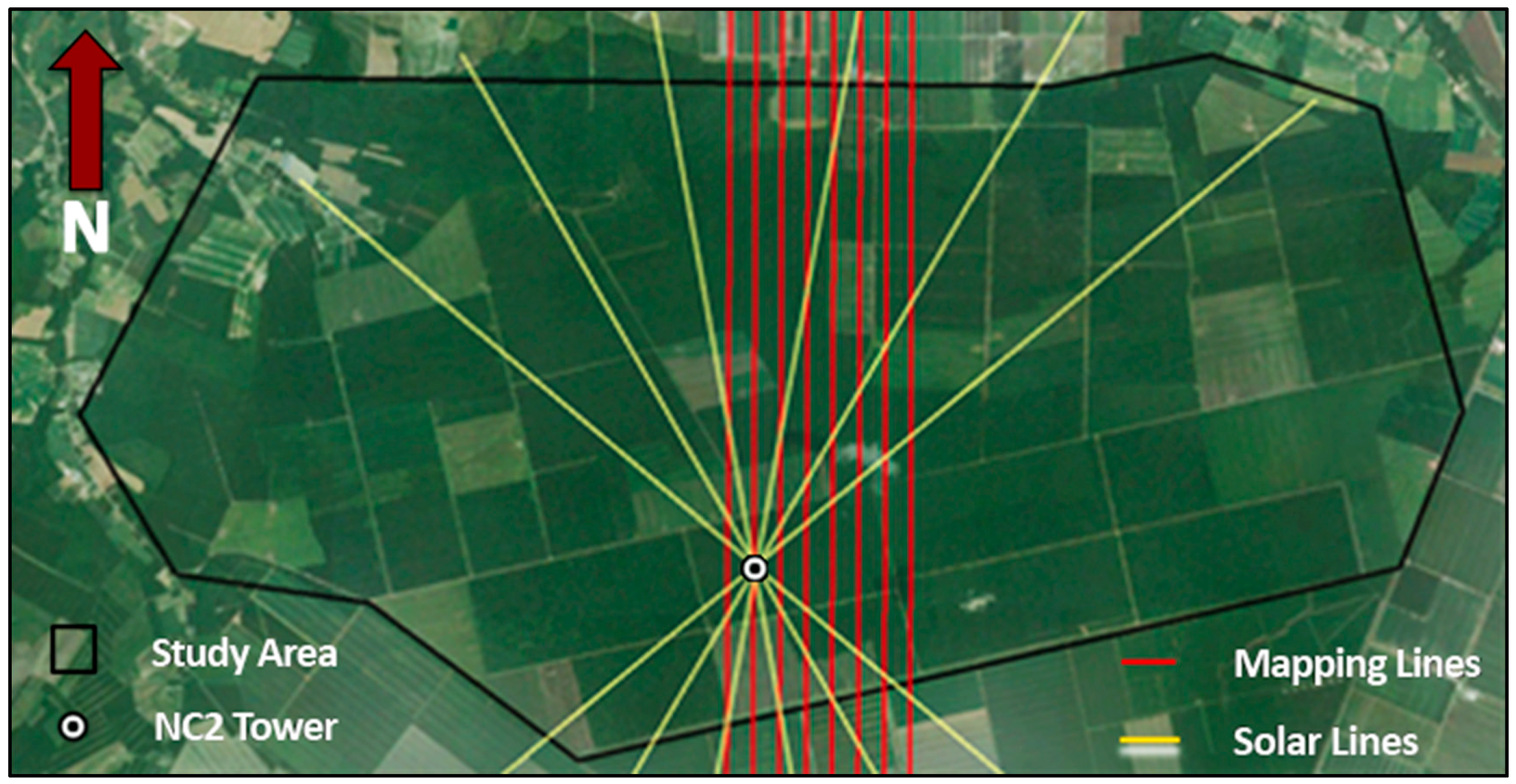
2.1. Site Description

The FLEX-US campaign reported here was conducted over the Parker Track Loblolly Pine (P. taeda L.) Plantation located on the lower coastal plain near Plymouth, NC, USA (35°48′N 76°40′W, Figure 1). The site is managed by the forestry industry for timber production, with an average growing season of 195 days. Loblolly pine (LP) is the dominant species with some mixed deciduous/coniferous old-growth and riparian forests. The area is flat, poorly drained soil with a ground elevation of 8 m above sea level. A network of drainage ditches and canals divide the watershed into a mosaic of regularly shaped fields on which different age classes (2–40 years in 2013) were artificially established by Weyerhaeuser Co. (Seattle, WA, USA) to provide distinct differences in forest structure. Forest biometry measurements and tower observations of atmospheric carbon dioxide (CO2), water vapor, and heat flux within the boundary layer have been collected at this site >10 years by Weyerhaeuser Co., NC State Univ., and the US Forest Service [8,9].

2.2. Aircraft Instruments

The HyPlant and G-LIHT instrument packages were co-manifested on the NASA UC-12B King Air research aircraft equipped with dual ports. Installation and certification were completed between mid-August and early September 2013 at NASA’s Langley Research Center (LaRC, Figure 2). Both instrument packages use the geographic positioning system (GPS) based inertial navigation systems (GPS/INS, Oxford Technical Solutions, Oxfordshire, UK) as a common solution. The GPS/INS data, along with rigidly mounted components, support high precision position and attitude measurements, enabling data fusion for coincident fine-scale products at 2 m resolution. The six-axis inertial navigation system, with three angular rate sensors (gyros) and three servo-grade accelerometers, incorporates a level 1/level 2 (L1/L2) GPS receiver with an OmniStar HP decoder to deliver 0.1 m positioning and 0.1° heading accuracies. Outputs from the system are derived from the measurements of the accelerometers and gyros using a 250 Hz data rate. GPS/INS data are stored on internal memory in a raw, unprocessed format which can be accessed via the data communications port.

2.2.1. HyPlant

HyPlant is a unique, custom high-performance imaging spectrometer system for airborne and ground-based vegetation monitoring [3] developed by the Forschungszentrum Jülich (Jülich, Germany) in cooperation with Specim Spectral Imaging Ltd. (Oulu, Finland). The sensor package operates in a push-broom mode and consists of two optical imaging modules: (A) the DUAL-imager, a line-imaging VSWIR spectrometer consisting of two sensors integrated in a single housing using a common fore optics to provide contiguous spectral information from 370 to 2500 nm, with 3 nm spectral resolution in the VNIR spectral range and 10 nm spectral resolution in the SWIR spectral range; and (B) the fluorescence imager (FLUO), a special module that acquires data at very high spectral resolution (0.25 nm) in the spectral regions of the two atmospheric oxygen absorption bands (670–780 nm) and is dedicated to measuring the vegetation fluorescence signal. HyPlant is supported with a position and attitude GPS/INS sensor, an adjustable mount, and a data acquisition/power unit which contains two rack modules. The first module supports the DUAL imager with a data acquisition computer having system control and data acquisition software, and with power supply and control electronics. The second module includes the same equipment for the fluorescence imager. The GPS/INS sensor provides aircraft position and attitude data to enable image rectification and geo-referencing. Both HyPlant imagers are mounted in a single platform with the mechanical capability to align the field of view (FOV). Descriptions and specifications of the HyPlant package and examples of typical spectra were described by Rascher et al. [3]. The HyPlant system was intensively tested during the ESA HYFLEX 2012 campaign [10], after which technical adjustments were made by Specim Spectral Imaging LTD (Oulu, Finland). Test flights were conducted in Germany during April 2013 to verify the updated performance, in advance of the FLEX-USA campaign.

2.2.2. G-LiHT

G-LiHT [4,5,6] is a portable, airborne imaging package comprised of commercial off-the-shelf (COTS) components to simultaneously map the composition, structure, and function of terrestrial ecosystems using scanning LiDAR, hyperspectral reflectance, and thermal imagers co-aligned along a uniform optical axis that is parallel to the flight path [11]. The components are: (A) a small footprint scanning LiDAR (VQ-480, Riegl USA, Orlando, FL, USA) to provide 3D information about the vertical/horizontal distributions of canopy elements; (B) the Hyperspec concentric imaging spectrometer (Headwall Photonics, Fitchburg, MA, USA) to enable VNIR imaging reflectance from 418 to 918 at 10 nm spectral resolution; and (C) a thermal imaging camera, Gobi-384 (Xenics, Leuven, Belgium), for surface temperatures and to detect heat/moisture stress based on a single 8–14 µm longwave infrared (LWIR) band. The system components are assembled into a rigid weather resistant enclosure with a compact volume of <0.1 m3 including the data acquisition sub-system for a total weight of 37 kg. The following sections summarize the details of how G-LiHT was configured to support this campaign. Further details can be found in the G-LiHT white paper [12].

Airborne Scanning LiDAR

The VQ-480 airborne scanning LiDAR is comprised of an integrated high-performance laser rangefinder (wavelength, 1550 nm) and a rotating polygon 3 facet mirror which deflects a Class 1 laser beam operating along a 60° swath perpendicular to the flight direction at a repetition rate of 150 kHz for this campaign, but accepts a user selectable repetition rate up to 300 kHz. The laser beam divergence is 0.3 mrad. The rotating speed of the multi-facet mirror is 100 scans/sec, to provide an angle measurement resolution of 0.001 degrees. Each laser measurement is time tagged and accurately related to the single solution GPS/INS system via a serial RS232 interface. The PC software RiACQUIRE (Riegl USA Inc., Orlando, FL, USA) provides a graphical user interface for scanner control and data acquisition with status feedback. Based on time-synchronized scan data, position, and attitude information, scan data coverage is calculated in real time to indicate point density coverage of the target area.

Imaging Spectrometer

The Hyperspec imaging spectrometer (Headwall Photonics, Fitchburg, MA, USA) is based on the Offner design and enables spectral VNIR (418–918 nm, 10 nm full width at half maximum, FWHM) imaging at high spatial resolution through high efficiency f/2.0 telecentric optics, a high efficiency aberration-corrected convex holographic diffraction grating, and a C-mount objective lens (Cinegon f/1.4 8mm, Schneider Optics, Hauppauge, NY, USA). The Hyperspec has operated on G-LiHT over a wide range of conditions, including harsh environments, providing stable radiometric results. The GSFC unit receives a full calibration annually at the GSFC Biospheric Sciences Laboratory’s Radiometric Calibration Laboratory which maintains US National Institute of Standards and Technology (NIST) traceable calibration sources and detectors, and is additionally monitored regularly for radiometric and wavelength stability using a portable Teflon integrating sphere with Tungsten Hg/Ar lamps.

Downwelling Radiometer

Downwelling radiance is measured using the Ocean Optics USB 4000-VNIR spectrometer, 350–1100 nm at ~1.5 nm FWHM (Dunedin, FL, USA). Light energy is transmitted to the spectrometer through an upward looking opaline glass cosine diffuser with an 180° FOV. A 3 m 100 µm optical fiber delivers the light energy through a 25 µm entrance slit and a multi-bandpass order-sorting filter. It then disperses via a fixed grating across a 3648-element Toshiba linear CCD array. Power and communications occur through a USB 2.0 connection to the central PC. The downwelling radiometer is operated continuously during flight with a 33 ms integration time averaged for 30 scans, and 3× spectral binning yields a 1 Hz data acquisition rate. The unit is radiometrically cross calibrated with the imaging spectrometer to enable atmospheric characterization of down welling irradiance that is used to provide a surface reflectance product.

Thermal Imaging

The Gobi-384 thermal imaging camera (Xenics, Leuven, Belgium) has a broad 8–14 µm LWIR spectral band. It is covered by the uncooled a-Si micro-bolometer detector array (resistive amorphous silicon, FPA) with 384 cross track pixels and a 30° FOV. This compact component measuring 72 × 60 × 50 mm uses a Gigabit Ethernet TCP/IP interface to deliver 16-bit radiometrically calibrated thermal imaging data at a 25 Hz frame rate to the central computer running the Xenith software and graphical user interface. Each image frame is coded with a PC timestamp synchronized with the common solution GPS/IMU system. Push broom thermal imagery for each flight segment is generated in post processing where several cross track rows are exported in a series co-registered with the imaging spectrometer. The thermal imagery has factory radiometric calibration for surface temperatures between −20 °C and 120 °C with a noise equivalent temperature difference, NETD > 50 mK to allow airborne operations over a diverse range of surface temperatures. Thermal calibration stability as a function of microbolometer operating temperature is verified against the GSFC Calibration Facilities blackbody for stable operation over the target temperature range of −5 °C to 85 °C.

2.3. Flights and Ground Support

FLEX-US airborne flights were flown over the Parker Tract site from September–October 2013. For the science flights, the nominal flight altitude was 600 m above ground level (AGL) with instrument FOV ranging from 35° to 60° and native ground sampling of 2 m. Flight profiles per observation period consisted of 8 N-S lines (shown in red, Figure 1) with 50% overlap to achieve high density mapping of a 12.5 km2 area within the boundary of the LP plantation. One of the eight flight lines that covered the area to be mosaicked also passed over the AmeriFlux NC2 flux tower (Figure 1). In addition to the N-S lines, two more flight lines at the beginning and conclusion of each collection (shown as yellow lines in Figure 1, totaling ten lines per measurement period) were flown in the solar principal plane (SPP) and also passed over the NC2 tower. Each collection of the 10 flight line pattern took ~45 min. Reported here are results from data collected with this pattern, repeated 4 times over a diurnal cycle, yielding morning (10:30 local time, 55° to 62° solar zenith angle, SZA), mid-day (13:15 local time, 48.5° to 50.9° SZA) and afternoon acquisitions (14:15 local time, 49.6° to 56.5° SZA; and 15:45 local time, 60° to 66.9° SZA) over two consecutive days (26–27 October). Ground based support included the AmeriFlux tower and related meteorological information gained from the instrumented tower (e.g., air temperature) located within the most mature LP stand.
A ground-based Fieldspec-4 VSWIR spectroradiometer (ASD, Inc., Boulder, CO, USA) was positioned over two m2 calibration tarps (20% and 5% reflectance) laid out on an open grassland field (lat. 35.873635, long. −76.658774), and paired with a multiband photometer (CE318-T, Cimel Electronique, Paris, France) to record the atmospheric transmissivity, for use in atmospheric corrections of the optical data. Ground-based optical data were collected continuously throughout the days (09:00 to 17:00) when flights occurred for calibration and validation purposes on the grounds of the NC Department of Agriculture Tidewater Research Station. The two calibration tarps were spread out on a lawn and ASD measurements of the reflected radiances were made during the flights over the tarps, along transects (lengths, 2× the width of the tarps) across the lawn, and across a nearby parking lot at 1 m intervals. A second ASD spectroradiometer made measurements of a white Spectralon calibration panel (Labsphere Inc., North Sutton, NH, USA) at 10 s intervals. The calibration panel was also measured with the spectroradiometer used for the tarp measurements after each measurement set, to enable cross-referencing. These two ASDs were also cross-calibrated in the laboratory before and after the campaign.
Surface temperatures were collected using a thermal gun (model 100L-LV, Everest Interscience, Inc., Chino Hills, CA, USA) in conjunction with the ASD measurements. Surface temperatures were also measured at a nearby pond. A hand held IRT device (Agri-Therm II, Everest Intersciences, Tucson, AZ, USA) and a portable calibration black body (Palmer Wahl, Asheville, NC, USA) were used to measure the temperature of selected ground targets to verify the accuracy of G-LiHT’s surface temperature products. Leaf area index (LAI) was measured using a LAI-2000 Plant Canopy Analyzer (Licor Inc., Lincoln, NE, USA) at 37 plots spanning a range of stands of known age, where measurements were taken along two 10 m transects (NE→SW, NW→SE). Within 1/10 acre plots, average tree height was determined using clinometers, tree diameter was measured at breast height (DBH at 1.30 m), and forest stand density with stem counts (Table 1). These descriptive statistics were used in conjunction with G-LiHT LiDAR canopy height model (CHM) and additional LiDAR metrics variables and imaging spectrometer data to select representative Regions of Interest (ROI), 120 m × 120 m forest stands cutouts, large enough to enable evaluation of aircraft data aggregated to a range of spatial resolutions, ≤84 m2.

2.4. Data Collections and Data Processing Procedures

2.4.1. Flux Data from the Parker Tract NC2 Tower

Carbon fluxes were measured using eddy covariance techniques at the US-NC2 flux tower. The 23 m tall tower is located in the LP plantation at 35.8031°N, −76.66791°W, where the trees around the tower were planted in 1992 [8]. Net Ecosystem Production (NEP) from flux tower measurements was partitioned into Gross Ecosystem Production (GEP) and ecosystem respiration [9,13]. We computed the daytime daily average incident photosynthetically active radiation (PARi) and GEP throughout the full 2013 year and examined these fluxes for the days during the week of the campaign at half hour intervals for the time period between 09:30 and 15:30, to represent the fluxes during the flights. We also used the temperature data acquired at the tower to provide air temperature (°C) during each flight line.

2.4.2. HyPlant Data

Preprocessing of HyPlant Data

Preprocessing of the HyPlant calibrated images was performed by Jülich team members using the software package CaliGeoPro (Spectral Imaging Ltd., Oulu, Finland). CaliGeoPro provides most of the functionality that is necessary for pre-processing, i.e., radiometric correction, georectification, correction for spectral smile and band broadening as well as keystone correction. It became clear during this campaign that pixel-cross talk and stray light in the HyPlant FLUO sensor affect the fluorescence retrieval. Therefore, the FLUO images were radiometrically calibrated and corrected for the point spread function using an algorithm developed in Jülich in collaboration with L. Alonso (U. Valencia). Additionally, it was decided to spatially bin data to increase the signal to noise ratio and to reduce pixel adjacency effects.

HyPlant Fluorescence Retrieval

A data-driven fluorescence retrieval method based on a semi-empirical radiative transfer formulation (as opposed to full-physics modeling) was used to obtain fluorescence from the high resolution HyPlant FLUO data. This retrieval method was first developed by Guanter et al. [14,15] and previously used for fluorescence retrieval from HyPlant FLUO in Rossini et al. 2015 [8]. Fluorescence was retrieved at the two peaks of the fluorescence spectrum, in energy units (W m−2 nm−2 sr−1). The red fluorescence peak is around 685 nm, while the far-red peak is located around 740 nm, thus we term the fluorescence retrievals of the HyPlant instrument at F685 and F740, respectively.
The data-driven fluorescence retrieval approach represents the measured at-sensor radiance spectrum as a linear combination of reflected solar radiance and fluorescence emission spectra. The reflected solar radiance is formulated as a linear combination of singular vectors (SVs), which are derived after performing a Singular Vector Decomposition (SVD) of a set of reference (fluorescence-free) spectra. The combination of the derived SVs is able to reproduce any fluorescence-free spectra. This data-driven formulation of the forward model avoids the explicit modeling of atmospheric radiative transfer and the instrument’s spectral and radiometric responses, which are typically prone to errors larger than the fluorescence signal itself. The SVs are derived using non-fluorescence training pixels, which are determined by a threshold on the Normalized Difference Vegetation Index (NDVI). We typically used 4–5 SVs to model the “at-sensor” radiance signal. A few adjustments were applied to improve the inversion results, such as the removal of the strongest absorption features or the spectral normalization (continuum removal) of canopy and reference radiances.

Surface Reflectance from HyPlant

Surface reflectance was calculated from calibrated “at-sensor” radiances measured with the HyPlant DUAL module by using the Atmospheric & Topographic Correction, ATCOR-4 (ReSe Applic. Schlӓpfer, Langeggweg, Switzerland) program for wide FOV airborne optical scanner data [16,17]. Atmospheric corrections were applied using atmospheric functions supplied from the MODerate resolution TRANsmission model (MODTRAN, Spectral Sciences, Burlington, MA, USA) [18,19]. Initial atmospheric parameters were estimated from sun-scan measurements, relying on reflectance measurements made of the tarps in each flight line to constrain the atmospheric correction. No correction for a digital elevation model was applied since the study area was very flat and thus no major topographic contribution of the 3-D surface was expected.

2.4.3. G-LiHT

G-LiHT Thermal Sensor

Surface temperature data products from G-LiHT’s LWIR thermal imager were generated for both individual flight lines and other mapped areas. This imager with its 384 cross track pixels and a 30° FOV has the narrowest swath and lowest cross track sampling of G-LiHT’s sensors and frequently dictates the flight line spacing to achieve continuous coverage. However, the surface is oversampled along track and typically 100 (along track) lines are extracted from each frame of the 25 Hz video sequence. Again, the fixed relationship between LiDAR scan angles and pixel centers is exploited through backwards projection to populate each co-registered raster grid cell of the final data product. Data were collected at the ground calibration site with a hand held IRT device and a portable calibration black body, as described above, to verify the accuracy of G-LiHT’s surface temperature products.

G-LiHT LiDAR

Customized LiDAR data processing code was written in IDL (EXELIS Visual Information Solutions, Boulder, CO, USA) to ingest the raw swath-based unfiltered LAS files from G-LiHT. Algorithms apply a grid-based bottom-up Delaunay triangulation process with a progressive morphological filter16. Lowest elevation points (i.e., ground returns) are isolated and used to create a Triangulated Irregular Network (TIN) from which the digital terrain model (DTM) is generated through interpolation to uniform raster grid spacing. The grid cell size is selected so each cell has a sufficient population of LiDAR returns which is proportional to flight altitude, laser repetition rate, surface complexity and reflectance at 1550 nm. Typical flight altitudes and laser repetition rates for G-LiHT are 300 m/300 kHz or 600 m/150 kHz, which yield 1 m or 2 m data samples, respectively. G-LiHT DTM products include ground slope and aspect, reported in degrees. Next, triangulation is used to determine the base elevation of every non-ground return and the Canopy Height Model (CHM) is created by selecting the greatest vegetation return height for every grid cell.
Commonly used statistical metrics are derived from the remaining LiDAR returns which fall between the modeled top of canopy and ground surfaces. These are subdivided into shrub and tree classes based on a threshold height (above ground value, 1.37 m). Statistical metrics are calculated based on a 14 m2 grid size such that a sufficient sample population is achieved for each grid cell. A total of 35 LiDAR metrics are included in the standard G-LiHT distributed data products which include: mean and standard deviation of all tree and shrub heights; tree fractional cover (fraction of first returns intercepted by tree); and tree return percentiles and deciles in 10% increments. A complete list of G-LiHT plot scale metrics are archived [20].

G-LiHT Headwall VNIR

The post processing of G-LiHT’s imaging spectrometer data consists of applying radiometric calibration coefficients to data from both the imaging spectrometer and the downwelling radiometer, effectively converting the raw digital number (DN) values to at-sensor upwelling surface radiance and downwelling irradiance, respectively. Normal G-LiHT operations occur at or below 600 m AGL and cross-calibration of the two instruments allows computation of the surface reflectance data product with minimal atmospheric effects. Imaging spectrometer spectral bands are aggregated from the 1.5 nm native sampling interval using a 3× pixel aggregation approach such that distributed hyperspectral data have 114 spectral bands between 418 nm and 918 nm, with 4.5 nm band spacing and a 10 nm FWHM spectral resolution. Swath based hyperspectral data cubes are provided for at sensor radiance (W m−2 nm−1 sr−1) and reflectance products.
Co-registration for G-LiHT’s data products is achieved by a “backward projection approach” from the LiDAR surface models. As G-LiHT sensors are rigidly mounted in a fixed orientation, the geometric relationship remains constant between the LiDAR scan angle and pixel centers of the push broom optical sensors. Each grid cell is populated with observations with the same angular view from each of G-LiHT’s optical instruments. If no coincident optical views are available to populate a grid cell then the nearest neighbor is used to ensure contiguous coverage. A record is retained as to whether a matching view (1) or a nearest neighbor (0) was used to populate the raster grid and this information is stored in an associated ancillary file. Geo-located optical data products (L1G) are available for a portion of these and other G-LiHT acquisitions at other sites, and can be accessed at: ftp://fusionftp.gsfc.nasa.gov/G-LiHT/.
In addition to G-LiHT’s swath-based products, mosaicked data products are automatically generated for mapped areas that have overlapping flight lines of the same heading. The IDL code that generates these products populates predefined grid cells from the LiDAR-generated surface model with the closest to nadir views available from the coincidently collected imaging spectrometer swath data. A record is retained in the ancillary image file indicating swath number and corresponding view angle for each pixel in the final data product. Further, a number of commonly used vegetation indices are generated including; NDVI and the Photochemical Reflectance Index (PRI). Further details regarding G-LiHT configuration and data products can be found in references [4,6].

2.5. Analyses

Analyses of these comprehensive datasets were conducted to enhance our understanding of ecosystem form and function in this managed coniferous forest. Flux tower data are summarized in Figure 3. We examined the impact of LP stand age and structure dependencies on spectral optical indices derived from fluorescence and reflectance measurements, and their use as bio-indicators of ecosystem LUE for a set of forest ROIs having discrete age classes, biomass and canopy closure. We provide examples of data collected at the native 2 m2 spatial resolution (Figure 4), data aggregated at 14 m2 in the standard G-LiHT format that was originally implemented for LiDAR (Figure 5, Figure 6 and Figure 7), and data which were aggregated to ~49 m2 (Figure 8, Figure 9, Figure 10, Figure 11, Figure 12, Figure 13 and Figure 14) to obtain representative values per ROI. These examples demonstrate the relevance of this type of data to science questions and characteristics of future satellite missions such as ESA’s FLuorescence EXplorer (FLEX, 2022 [1,2]) and the NASA Pre-Phase A concept Hyperspectral Infrared Imager (HyspIRI) [21].
Imagery from both the G-LiHT VNIR spectrometer and the HyPlant DUAL VSWIR spectrometer were used to compute two well-known normalized difference spectral reflectance (R) indices: the PRI (e.g., [22,23,24]), and the NDVI (e.g., [25,26]), where the standard PRI = [(R531 − R570)/(R531 + R570)] and the NDVI = [(R750 − R660)/(R750 + R660)], using 5 nm bands. The HyPlant DUAL Spectrometer data were also used in conjunction with accepted spectral algorithms to derive canopy parameters such as leaf area index (LAI) and total canopy chlorophyll (TChl) content. TChl was estimated using the MERIS Terrestrial Chlorophyll Index, MTCI [27,28], which was developed as a standard ESA product for the Medium Resolution Imaging Spectrometer (MERIS), where MTCI = [(R754 − R709)/(R709 − R681)]. The red/far-red fluorescence ratio (Fratio), F685/F740, was computed from the HyPlant FLUO. This ratio has been used to describe photosynthetic efficiency at leaf level (e.g., [29,30,31]) and canopy level (e.g., [32,33]).
Analyses focused on fluorescence and reflectance variables for the ROI stand age groups (n = 30) across the Parker Tract forest site. For the mature stand associated with the AmeriFlux NC2 tower, analyses examined the comparisons of tower-estimated LUE (GEP/PARi) and optical variables derived from HyPlant’s FLUO fluorescence and DUAL reflectance data. Statistical analyses were conducted with Systat 13 (Systat Software, Inc., San Jose, CA, USA).

3. Results

3.1. Data Collections at High Spatial or Stand Level Resolution

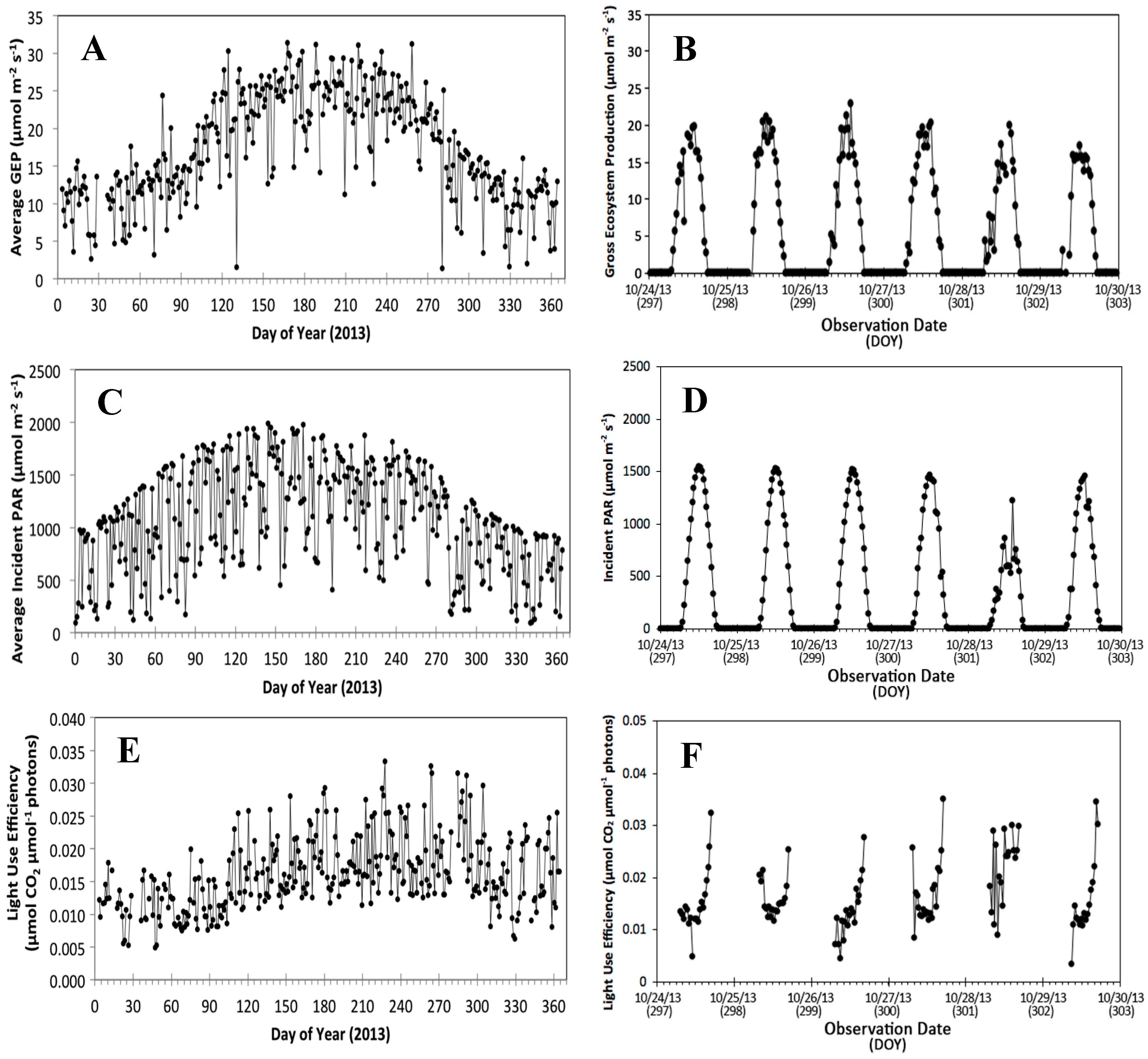
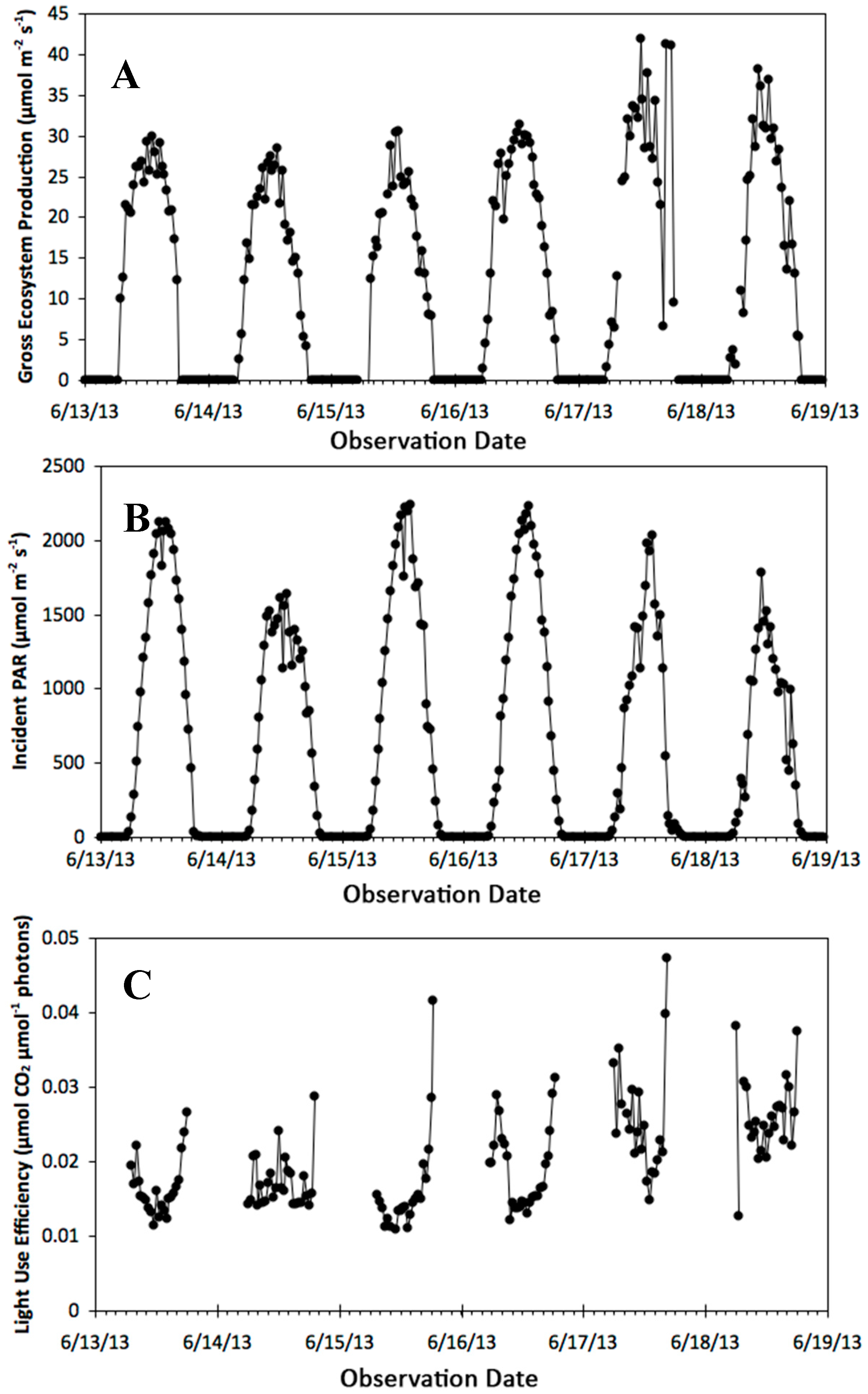
3.1.1. The NC2 Flux Tower

For this study, daytime average incident PARi and GEP were calculated for the time period between 09:30 and 15:30, to represent the fluxes during the flights, for all days over the entire 2013 year (Figure 3A,C). In these data series there is significant variability from day to day, with a summer maxima for daily averaged GEP of 31.2 µmol CO2 m−2 s−1 on DOY 188 (7 July); and a PARi maximum of 1981 µmol m−2 s−1 three weeks earlier, on DOY 170 (19 June). The daily averaged fluxes at the time of the FLEX-US campaign flights (26–27 October) were approximately 50% of the summertime maximum GEP (16.8 and 16.6 µmol m−2 s−1, respectively) and approximately 60% of the maximum PARi (1231 and 1162 µmol m−2 s−1, respectively).
We examined the diurnal change in GEP and PARi within the days of the flights, as well as for two days before and after the campaign (Figure 3B,D), at half hourly intervals. Photosynthetic light use efficiency (LUE) calculated from tower fluxes as GEP/PARi shows a strong diurnal variation with noontime LUE values of 0.013 µmol CO2 µmol−1 photons on both of the flight days, with LUE increasing into the afternoon to achieve much higher values, 0.036 µmol CO2 µmol−1 photons (Figure 3F). For this coniferous evergreen site the daytime average LUE varies widely from day to day, mirroring irradiance, but the daytime averages for LUE during the October flight days were not significantly different from midsummer values (Figure 3E).

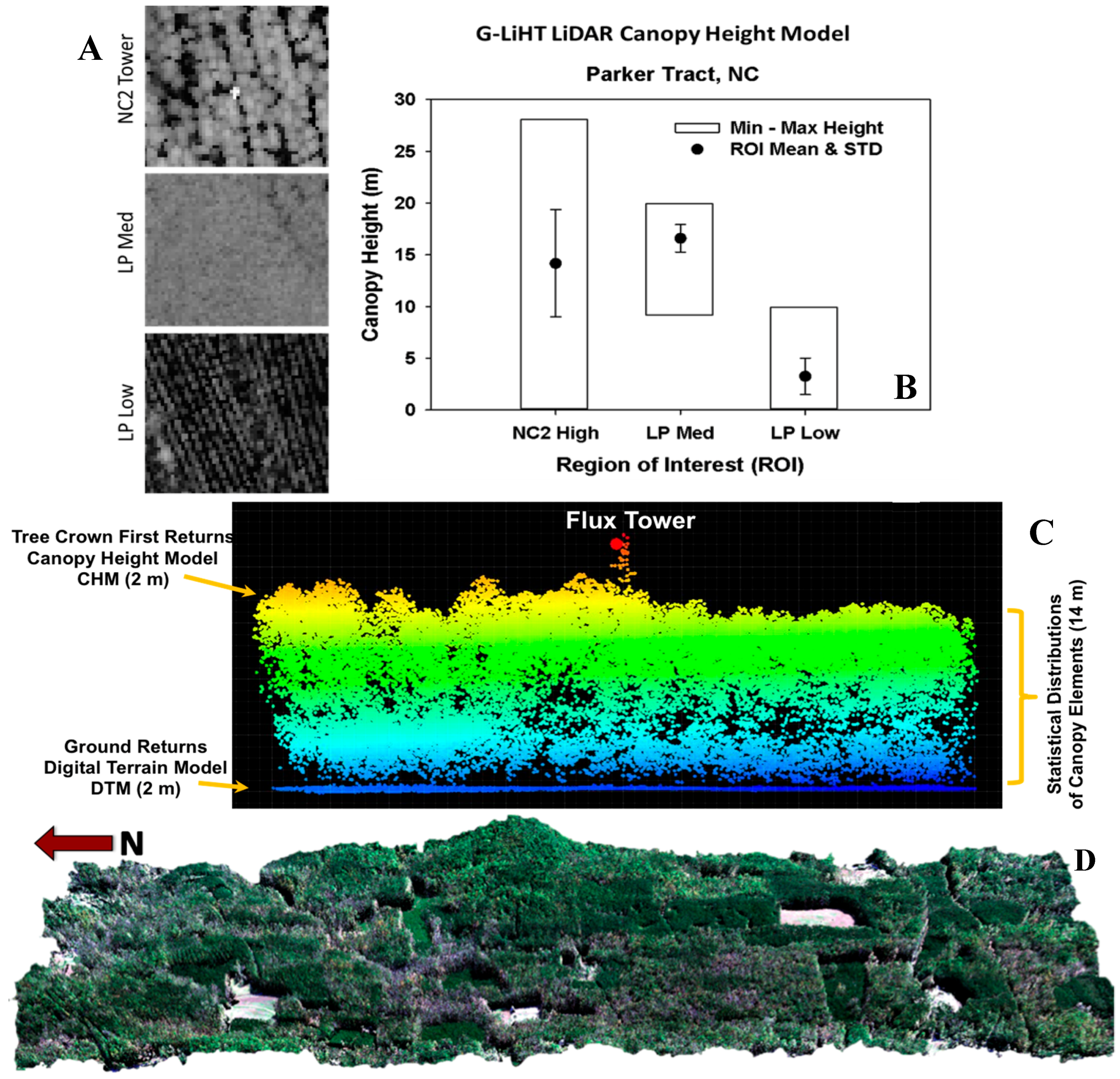
3.1.2. Canopy Structure

The stand canopy heights were determined using the G-LiHT LiDAR Canopy Height Module (CHM) data (2 m), averaged over several overpasses of the Parker Tract study site. Based on their average CHM values (for each of the 30 ROI cutouts), the LP stands were assigned to one of three height categories: low (≤9 m with open canopy, LP low), medium (10–20 m with a dense closed canopy, LP Med), and high (≤27 m with closed canopy, NC2 Tower) (Figure 4), which was verified with point measurements of tree height, DBH, canopy LAI, and density. Figure 4A,B provides examples of the 120 m × 120 m ROI cutouts within representative stands for the 3 height categories, with the mean ± SD (and maximum/minimum values) per category. A side view of the geo-referenced point cloud is provided in Figure 4C, where first returns from tree crowns (@ 2 m) were processed through the CHM (yellow layer) and the ground-level returns (blue layer) were determined with a Digital Terrain Model, DTM. Other LiDAR information that is computed includes surface rugosity (SD of CHM @ 2m), tree fractional cover (14 m), and the distribution of canopy elements (Deciles & Percentiles @ 14 m). Also shown in Figure 4D is a graphic example of the fine scale co-registration of G-LiHT’s data products, where the RGB optical image of the Duke Forest study site is overlaid on the LiDAR digital elevation product.
We note that FLUO data acquired in this campaign provided critical information that led to corrections for instrument signal effects that affected the usage of the highest resolution (2 m) data, subsequently rectified by the manufacturer (Specim, Inc., Oulu, Finland).
The ROI cutouts were separately analyzed at the 14 m2 spatial resolution described by the G-LIHT data products, from which a relationship between canopy height, stand age, and red fluorescence was successfully developed and reported elsewhere by Colombo et al. [34].

3.1.3. Thermal Data

Data collected at the ground calibration site with a hand held IRT device and a portable calibration black body verified the accuracy of G-LiHT’s surface temperature products (Figure 5). Here differences in radiant energy between morning and mid-day acquisitions along with imaging spectroscopy data were used for ecosystem assessments of Gross Ecosystem Production (GEP) and LUE, discussed in later sections.

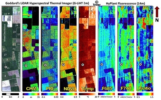
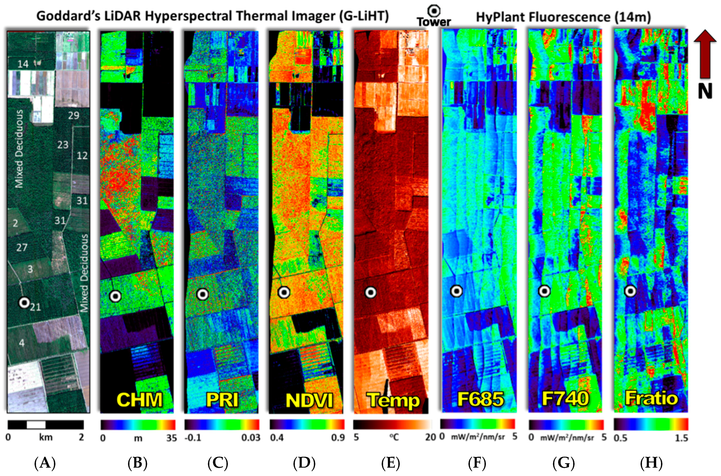
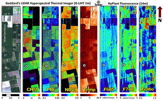
3.1.4. Individual Map Products

Mosaics for eight types of individual map products were made for these variables: CHM, RGB reflectance, the surface temperature from G-LiHT observations, and fluorescence retrievals from HyPlant FLUO (Figure 6A–H). The original high resolution ~2 m sampled data obtained from the flight lines (red lines, Figure 1) were aggregated to 14 m2 spatial resolution in these map mosaics. Mosaics were constructed from data obtained from the parallel N-S flight lines during a single solar noon collection (26 October, centered on midday 13:15 local time, ~solar noon) that covered a ~45 min time period during which the aircraft was systematically moving from the west side to the east side of the designated campaign subarea of the Parker Tract forest.
Map products derived from the G-LiHT VNIR spectrometer include the RGB image from the VNIR imaging spectrometer (Figure 6A), and several spectral reflectance indices, including the PRI and the NDVI (Figure 6C,D). Also obtained from G-LiHT were the CHM estimates derived from LiDAR data (Figure 6B), and the adjusted surface temperature, °C (Figure 6E). Map products from the HyPlant FLUO module included the red-band fluorescence emissions derived at 685 nm (F685), the far-red fluorescence emissions derived at 740 nm (F740), and their red/far-red fluorescence ratio (Fratio), F685/F740 (Figure 6F–H). The spatial patterns for the VNIR and thermal data were relatively smooth across their mosaics, being relatively unaffected by the changing illumination conditions (e.g., solar zenith and azimuth angles) over the <1 h flight period. The thermal patterns were best for identifying fallow vs. standing vegetation. In contrast, the fluorescence spatial patterns were highly responsive to the changing illumination conditions, such that the merging of flight lines at this resolution scale still retained delineated features related to flight lines. These were due to the within strip scanning views (nadir ± 10°) and the west to east progression of the N-S flight strips while both the SZA and the solar azimuth were changing. This is most evident for the earlier flight lines, which are located on the left side of each fluorescence mosaic (Figure 6F–H), when the solar angles were changing the most rapidly.
For this dataset, the age class patterns shown in the image (Figure 6A) are retained in the CHM, the PRI, and the NDVI mosaics (Figure 6B–D), and to a lesser extent in the thermal image mosaic (Figure 6E). In this particular mid-day example, the age classes were not well discriminated with fluorescence variables.

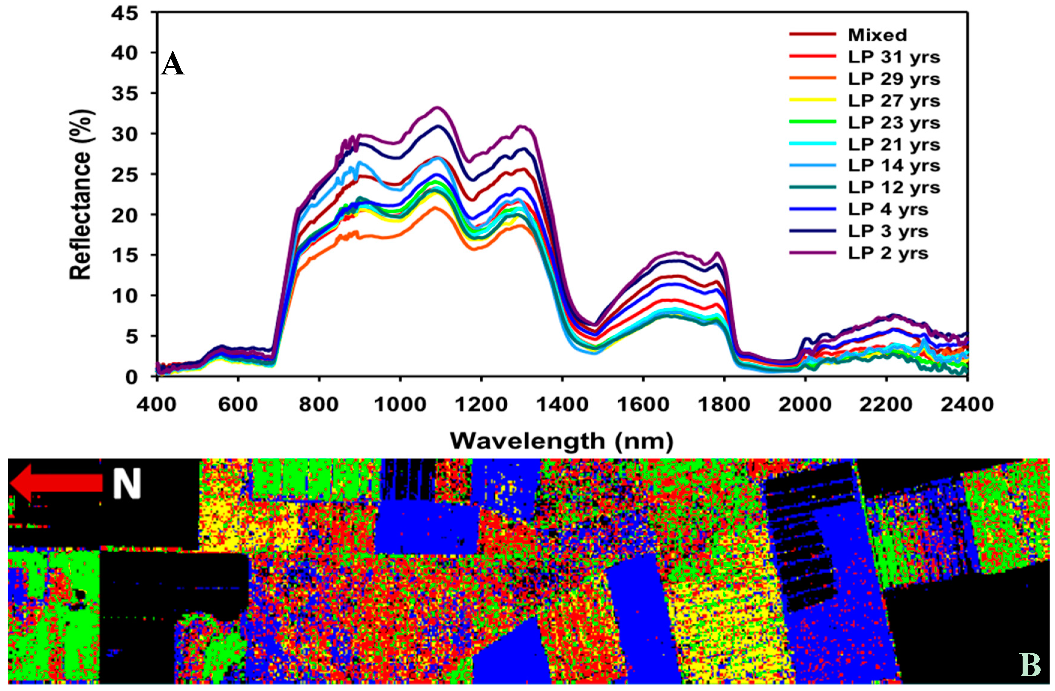
3.1.5. HyPlant DUAL VSWIR

The capability of the HyPlant DUAL VSWIR spectrometer to discriminate forest classes was evaluated at the native 2 m spatial resolution, since this instrument enables full spectrum reflectance observations acquired with high signal to noise ratio (SNR). As expected, The HyPlant DUAL provided excellent discrimination of LP forest stand ages, which was apparent with the range of reflectance magnitudes across the VSWIR spectrum (Figure 7A), especially in the NIR (~760–1300 nm), the MIR (~1500–1800 nm), and even the SWIR (~1900–2400 nm) regions. The visible range (400 to ~700 nm) provided little age class discrimination. The LP ROIs generally sorted out according to stand age, with the younger stands having higher NIR, MIR, and SWIR reflectance and the older stands displaying lower reflectance across the entire VSWIR spectrum. For example, the youngest (2 year) age class exhibited the highest NIR reflectance (~30–35%), whereas the mature 29 year class had the lowest NIR reflectance (~15–20%), with the intermediate age classes falling in between (Figure 7A). The oldest LP group (33 year) didn’t have the lowest NIR reflectance, but fell within the cluster of overlapping spectra for older LP stands (14–27 year). The spectrum for the mixed pine/deciduous group, which was visibly undergoing early stages of fall senescence with foliage color changes, fell between the spectra for the 3 and 4 year old LP classes.
When the mosaics made from the HyPlant DUAL VSWIR spectra and the G-LiHT CHM were merged at this spatial scale (14 m2)(Figure 7B), it was possible to discern smaller scale spatial patterns in the mosaic than were seen in the comparable maps of PRI and NDVI from the G-LiHT VNIR spectrometer (Figure 6C,D). This merged HyPlant/G-LiHT (VSWIR/CHM) product enhanced interpretation of the site’s spatial distribution of stand age classes and complements G-LiHT’s CHM/RGB 3-D mosaic (Figure 4, bottom).

3.2. Aggregating Data to 49 m2

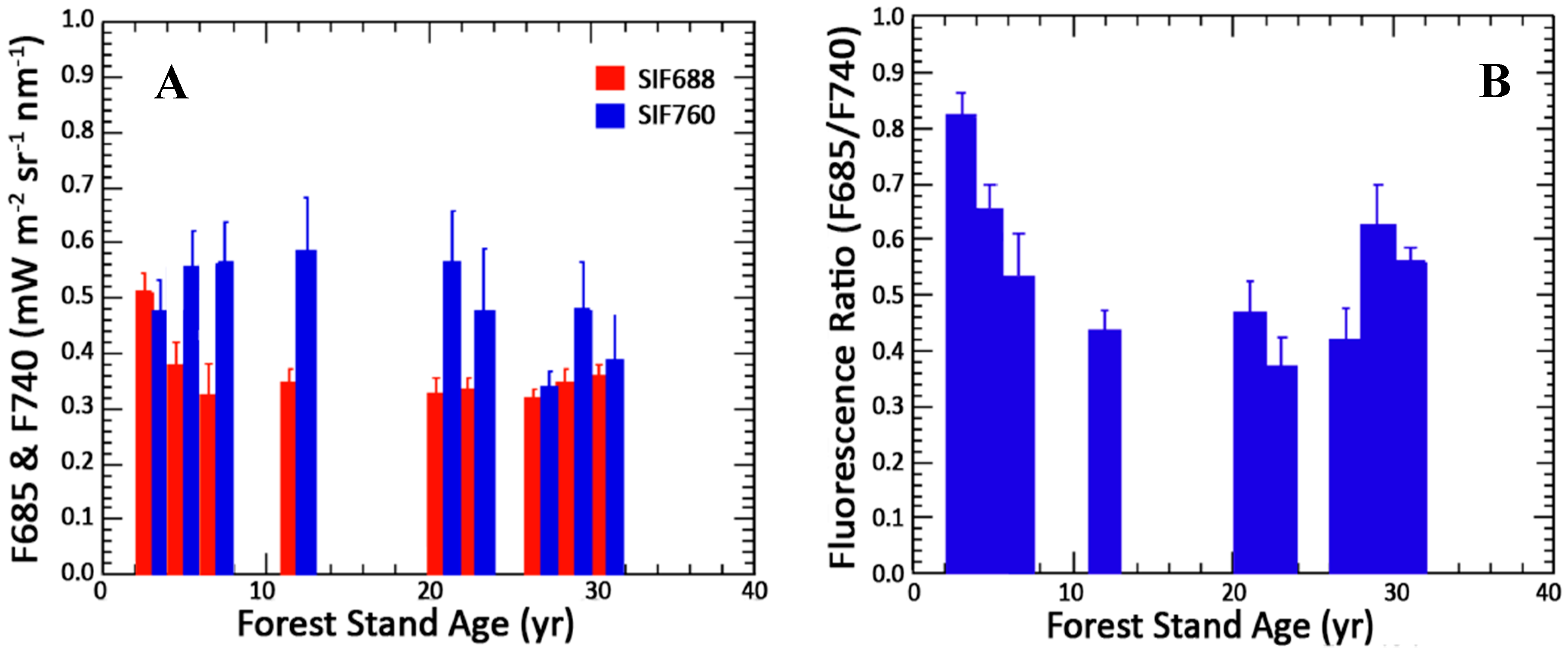
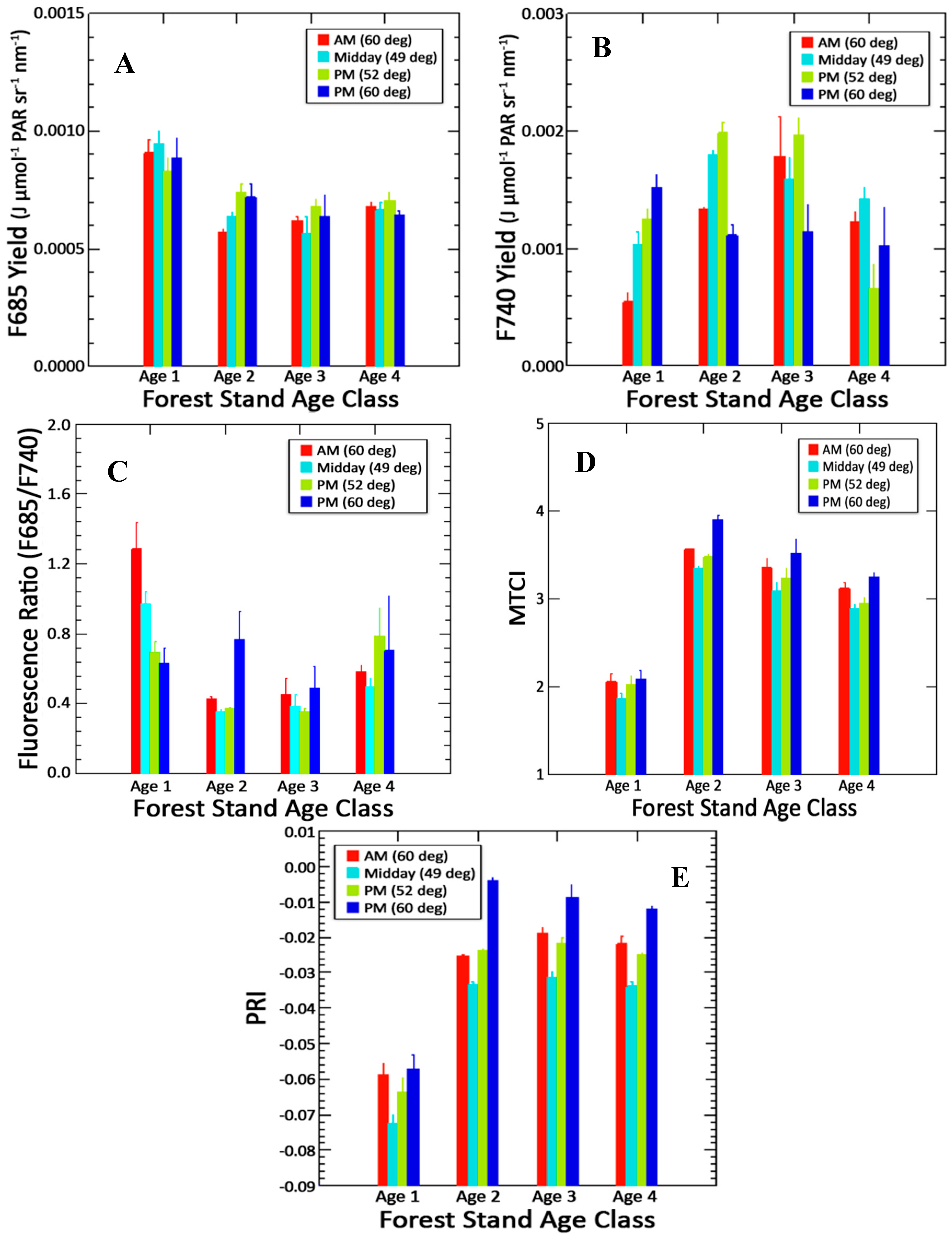
3.2.1. Fluorescence Group Means for Age Classes and Time Periods

The products described in Section 3.1 were aggregated within the ROI cutouts to a coarser spatial resolution (49 m2) to minimize the across track effects due to illumination changes that occurred during the 45 min long collections. This aggregation also minimized sensor noise/artifacts to enhance SNR, allowing us to explore statistically relevant relationships among variables.
We found that stand heights derived from LiDAR CHM data at this coarser spatial resolution (more suitable for satellite validations) were highly correlated (r = 0.97) with age class across the 33 year span of the ROI stands selected from the LP chronosequence at this site. At this spatial resolution, the fluorescence emissions for F685 decreased with LP stand age (Figure 8A) between 2 and 10 year old stands to a lower, steady average (0.3–0.4 mW m2 sr−1 nm−1) for the next 17 year stand age span. The far-red F740 was more variable across age classes (0.35–0.68 mW m2 sr−1 nm−1), and exhibited higher values associated with stand ages ≤23 year, than for the oldest stands. Consequently, the red/far-red Fratio (F685/F740) was bowl-shaped, expressing a minimum value (~0.4) between 10 and 22 years (Figure 8B).
The impact of the illumination changes associated with the four diurnal collections during the 2-day experiment, which occurred at SZAs of 60° in the morning, 49° around solar noon, and 52° and 60° in the afternoon, was evaluated by averaging the fluorescence values obtained for all stands at each time period (Figure 9A). These fluorescence responses show that the average F740 > F685 at each time period, with the highest daily mean fluorescence values at midday for both red and far-red fluorescence, 0.75 and 0.48 mW m2 sr−1 nm−1, respectively.
These data were further examined within the four time periods for four age group ranges (2–5 year, 12 year, 20–23 year, and 27–33 year) (Figure 9B,C). It is obvious that although F685 (0.25–0.80 mW m2 sr−1 nm−1) was typically lower (with exceptions) than F740 (0.3–1.3 mW m2 sr−1 nm−1), the highest F685 was produced from the youngest age group (red bars) across all four observation time periods. The F685 radiance was also less variable across age classes than F740 (Figure 8A,B and Figure 9B,C).
In addition, we observe that the youngest group (2–5 year) maintained higher F685 yields throughout the diurnal cycle than the older stands (Figure 10A,B), while the opposite trend was apparent for MTCI across age groups, with the lowest TChl estimate obtained for the youngest age class (Figure 10D). In contrast to F685 yields, the F740 yields (Figure 10B) were more diurnally variable than F685 yields. The far red fluorescence by itself has been related to photosynthesis or GPP (e.g., [31,32,33,35,36]). The Fratio, which has been shown elsewhere to be inversely related to photosynthetic efficiency [32,33,35], but also being greatly influenced by canopy structure, varied across the stand age groups Figure 10C. This bar chart indicates that the Fratio declined throughout the diurnal cycle in both the youngest (2–5 year) and oldest (≥27 year) age groups. A generally similar but reverse trend is expressed with the PRI (Figure 10E) which has also been proposed as a proxy for LUE or gross primary production, GPP (e.g., [22,23,24,32,33,35,37,38,39]). However, it is also well known that the PRI is greatly affected by canopy structure, and light absorption within the canopy, thus the significance of PRI—photosynthesis relations must be interpreted with care [35].

3.2.2. Combining Data Types

The PRI, commonly assumed to be associated with a subset of the carotenoid pigment pool, the xanthophylls (e.g., [37,38,39,40,41,42,43,44]), was strongly correlated during early senescence with canopy TChl content estimated with MTCI (Figure 11A, r2 = 0.96). Age class did affect this relationship: the lowest values for both the TChl and PRI (indicating lower TChl and higher stress) were obtained from the youngest age group, with slightly offset linear relationships for the two intermediate age groups (12–27 year). In addition, the PRI relationship to F685 was clearly different for young stands vs. older stands (Figure 11B), producing an overall highly significant inverse non-linear relationship (r2 = 0.90).
The PRI was also strongly and positively affected by temperature difference (air minus canopy, °C) (Figure 12A) (r = 0.98), also producing separate curves for young vs. older stands. Consistent with these results, we observed an overall inverse correlation (r = 0.80) of F685 over the diurnal cycle with this temperature variable Figure 12B). Notice that the hysteresis of the daily temperature gradient/cycle (shown with arrows) is noticeably amplified in the young open stands that have less foliage, lower TChl, and more surface background influences than older stands, and is compatible with trends given in Figure 9B. However, no consistent relationship for F740 with this temperature variable was obtained (Figure 12C).
In examining solar-induced fluorescence and LiDAR variables together, the only notable but weakly expressed relationship obtained at this spatial scale was for F740 as a function of the canopy Vertical Distribution Ratio (VDR), which had an overall r2 = 0.36 (p < 0.000, n = 139).
One of the successful results for this campaign—for one of the older mature forest stands—was the confirmation that the Fratio and the tower-based LUE (GEP/PARi, µmol CO2 µmol−1 photons) were strongly and linearly related (r2 = 0.84, all data with two time period categories). However, the Fratio vs. LUE relationship differed markedly for the midday collection when LUE response was flat and very low (cf., Figure 3F) vs. the combined morning/afternoon collection which spanned a large range of tower-acquired LUE conditions (Figure 13A). Therefore, the combined midmorning/afternoon set (blue curve in Figure 13A, n = 19) produced an even higher dependence of the Fratio on tower LUE (r2 = 0.91; SEM = 0.062), where the Fratio (AM, PM) = −0.500 + 33.75 × LUE. In contrast, only a moderate dependence of the Fratio on LUE was obtained at midday (r2 = 0.58, SEM = 0.10; Fratio (midday) = −7.52 + 372.51 + LUE. The influence of the canopy temperature difference (canopy-air, °C) on canopy LUE was more complex (Figure 13B), being strongly expressed in the morning when the temperature difference was greatest (1–2 °C) and less so in the two afternoon collections (0–1 °C) which displayed different slopes, but not strongly expressed at mid-day when the canopy and air temperatures were essentially equal (0 ± 0.4 °C). Given this context, the Fratio vs. LUE relationship was simpler (Figure 13A) and adequate for capturing the diurnal dynamics. For this combined midmorning/afternoon observation set, GEP could also be estimated in a multivariate analysis with three remote sensing variables (Figure 13C): PRI (p < 0.000), NDVI (p < 0.000), and F685 (p = 0.004) which produced an adjusted coefficient of determination, r2 = 0.75 (SEM, 1.303 µmol CO2 m−2 s−1, n = 34).
We further investigated the spectral data from the NC2 tower site, and confirmed that the red fluorescence was strongly and inversely related to the PRI (Figure 14A) as discussed earlier. The diurnal hysteresis with this pairing is readily apparent, increasing from the lowest F685 coupled with the highest PRI values during the morning collection to the highest F685 coupled with the lowest PRI values at midday. These responses reversed during the afternoon, finally returning to values similar to those in the morning set. Therefore, we reexamined this behavior for all stands, as previously shown in Figure 11B. Here, we separate the stands into young and older groups (and reverse the axes) but now the hysteresis for the combined stress response cycle expressed by the pairing of PRI with F685 is even more evident (Figure 14B). For the data cluster associated with the older stands (right cluster, Figure 14B), the highest PRI (~−0.01) was observed in mid-morning, then moved lower to −0.04 by noon, recovered to between −0.02 and −0.03 in early afternoon, and finally achieved values near zero by late afternoon. Comparable F685 (mW m−2 sr−1 nm−1) responses were: morning, 0.22 to 0.4; noon, 0.4 to 0.52; with recovery initiated in early afternoon, 0.28 to 0.45; and lowest values in late afternoon, 0.18 to 0.34. For the young stands (left cluster, Figure 14B), the PRI values are much lower (−0.04 to −0.08) and the F685 values are higher at midday, reaching 0.74 mW m−2 sr−1 nm−1. The hysteresis trends were similar for all canopy ages, but the beginning/end points within the diurnal cycle for the PRI were very different for young vs. older stands. Values for both PRI and F685 at the later afternoon period indicate recovery from stress. It is unlikely that diurnal TChl changes could produce this hysteresis effect. Note that it would be difficult to develop a relationship between F685 and PRI at any single time period, but that the relationship between these two small signals is evident when all four time periods are examined together, whether examining the oldest stand by itself (Figure 14A) or all canopies (Figure 14B).

4. Discussion

This paper describes results from a unique airborne campaign (FLEX-US 2013) conducted at the Parker Tract Loblolly Pine Plantation (Plymouth, NC, USA) study site [8] as an initial ESA-NASA collaboration to support ESA’s FLuorescence EXplorer (FLEX) mission [7]. This effort combined capabilities of multiple passive optical, active LiDAR, and thermal measurements, at a well-characterized study site having both an age class chronosequence and an AmeriFlux eddy covariance tower. The results from this airborne campaign demonstrate that the combined spectral information from chlorophyll fluorescence, reflectance spectroscopy, and canopy temperature—enhanced with structure measurements derived from LiDAR—can successfully discriminate canopy age and physiological response categories. Our campaign produced strong evidence in support of the utility of these combined measurement types. This was achieved for a LP forest, even though coniferous forests are known to have relatively low fluorescence emission. We obtained these results during autumn when environmental conditions are associated with lower irradiance and temperatures, with commensurate lower physiological activity, associated with this season in mid-latitude ecosystems. We may have been fortunate to capture the forest when a range of changes in canopy physiological conditions was taking place. Future studies are needed, and it will be important to obtain diurnal observations from different types of forests and other ecosystems over the full growing season, especially to compare the potential for the measurement sets used herein during the fall senescence with similar measurements obtained during summertime in conjunction with peak photosynthetic activity and high canopy chlorophyll content.

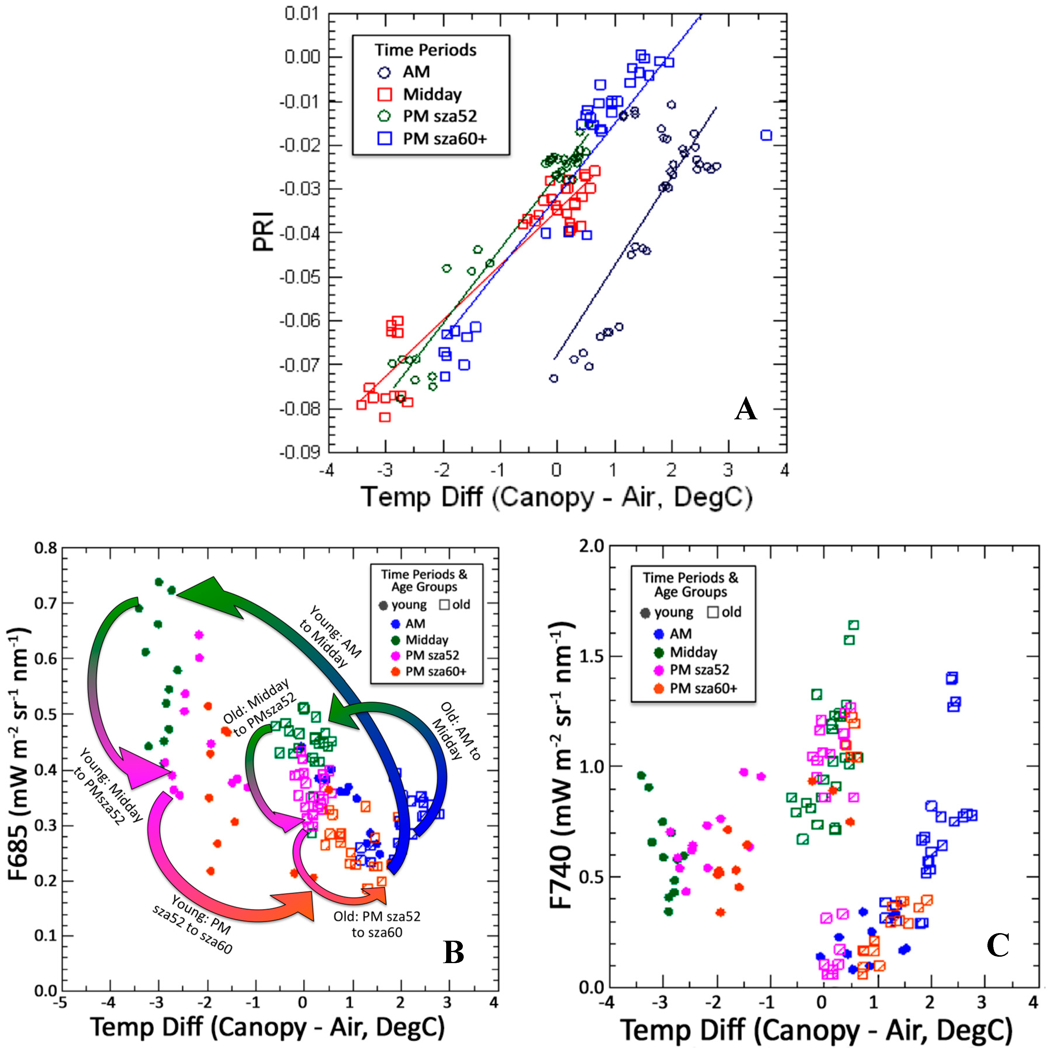
4.1. Fluorescence and the Canopy—Air Temperature Difference
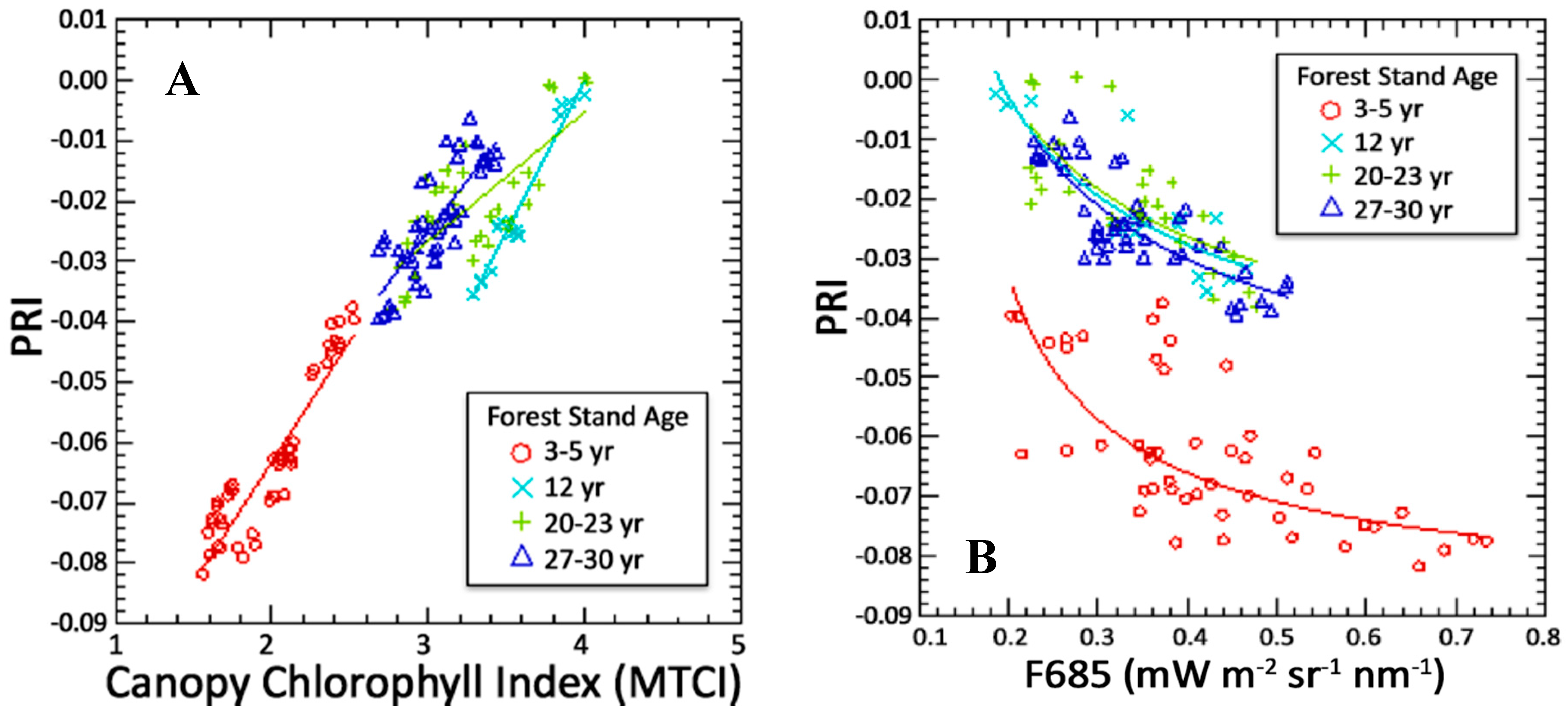
Our main findings were that forest stand age classes and diurnal processes significantly affected the emitted fluorescence within a LP forest. As reported previously by many researchers, the far-red fluorescence radiance (F740) was generally higher than red fluorescence (F685) across all age groups and throughout the observed diurnal cycle. However, F685 radiances (and/or F685 yields) provided a more reliable indicator of stand age, canopy chemistry, and physiological status than F740 radiances (or F740 yields), and was stable over older aged, closed canopy stands. This conclusion was also reached in a sister study for this campaign [34]. However, F685 radiances were non-linearly affected by the forest temperature difference (canopy-air, °C) throughout the diurnal cycle. All LP age group stands showed this hysteresis response—an increase in red fluorescence from mid-morning to midday, with a return to original values in mid-afternoon. However, the amplitudes of the fluorescence and temperature changes, driven by the daily irradiance regime, were especially pronounced in young, open stands (Figure 12B). The young stands, as compared to older stands, exhibited relatively low TChl and PRI values, coupled with higher F685 yields and Fratios. We note that thermal effects on the PRI and chlorophyll fluorescence have been studied in olive groves [45,46] and other field studies [47].

4.2. The PRI

Unlike the red fluorescence, the PRI was positively correlated to the canopy-air temperature difference. The PRI responded to canopy-air differences similarly for young and older stands, but with an offset for the morning observations when canopy-air temperature differences were ≥ zero (Figure 14A). This early morning observation presumably occurred before the protective xanthophyll pigment cycle was invoked by higher PARi and canopy temperatures that occurred by midday and were sustained until late afternoon. We also document that the Fratio and the PRI displayed opposite trends across the stand age range, and that the PRI displayed a stronger and direct relationship to TChl (as estimated with the MTCI) than did the inverse relationship for F685yield vs. TChl. In this coniferous forest undergoing early autumn senescence, very low PRI values in conjunction with F685 (e.g., Figure 11B) might be assumed to indicate time periods of higher stress, especially in the young stands. Together, the PRI and F685 were diagnostic for expression of physiologic down-regulation of photosynthesis in this forest (Figure 14B). The PRI has been identified as a superior spectral index for discriminating and tracking plant stress [47,48,49,50,51,52]. The combined use of PRI and fluorescence has previously been proven to be advantageous for plant stress detection [32,47,48,49,50,51,52]. We also note the recently reported [53] success in relating PRI (MODIS PRI, computed from bands of the Moderate Resolution Imaging Spectrometer on the Terra and Aqua satellites) to forest LUE using morning and afternoon observations from MODIS Terra and Aqua satellites at four coniferous and mixed forest sites in Canada.

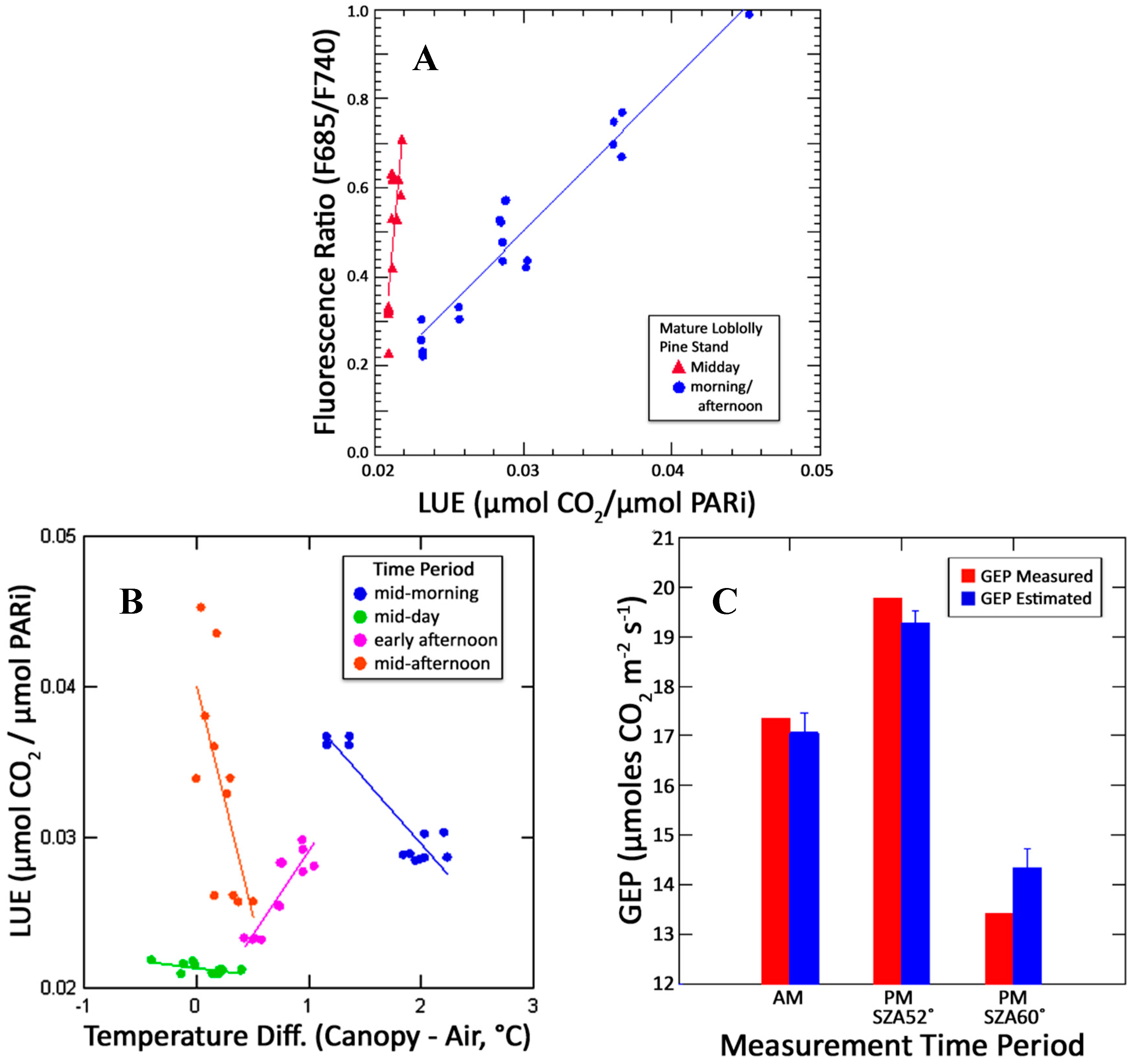
4.3. The Fluorescence Ratio and LUE

A valuable finding was that the red/far-red Fratio was successful for describing diurnal changes in canopy LUE at the mature stand where the NC2 tower was situated (r2 = 0.84 overall), with separate curves for midday (r2 = 0.58) vs. morning/afternoon (r2 = 0.91). The midday observations, when both canopy LUE and the Fratio changed rapidly, produced a steep slope with a separate cluster of midday observations (Figure 13A). Therefore, this was obscuring the underlying relationships when the midday observations were included with the combined morning/afternoon set. With the midday observations separated from the combined morning/afternoon datasets, a very strong relationship between the Fratio and canopy LUE was obtained (r2 = 0.96, one outlier removed). The red/far-red Fratio has been successfully related to canopy LUE in field campaigns previously [32,33,35] and has been used to improve forward modeling of GPP [54].
We investigated whether the midday LUE plateau observed in October (Figure 5F) also occurred during the summer 2013 peak production period, and substantiated that the midday LUE plateau was also often characteristic of midsummer diurnal responses (Figure 15A–C). In retrospect, this is expected given the hysteresis behavior of all light and temperature driven vegetation physiological responses (e.g., GEP, water fluxes, solar-induced fluorescence) that increase during mornings and decline during afternoons, as they pivot around the maximum achieved midday value. Therefore, it is apparent that a midday instantaneous collection (by itself) may not be the optimal time period for accurate estimation of LUE from airborne remote sensing using fluorescence (Figure 13A). Here, the Fratio increased drastically (~0.4 units) over a small increase in LUE (~0.03 µmol CO2 µmol−1 photons). It was also not possible to estimate GEP from these (or any) spectral variables at midday, given the small range of GEP observed during the solar noon time period, and since fluxes were reported at half-hourly intervals.
This new understanding may help explain the different results reported in the literature for experiments and campaigns conducted primarily in midday. Midday (cloudless) observations have been preferred as the ideal remote sensing measurements for the practical reasons of increasing SNR for passive optical instruments. These daily maxima are more accurate for estimating diurnal (i.e., total) carbon/water/thermal fluxes, as well as providing superior land cover classification maps from orbital sensors. However, in practice, and because field measurements are time-consuming, “midday” measurements often actually span a wider set of conditions on either side of solar noon, possibly blurring interpretations. Because midday observations (by themselves) display little variation, the observations acquired on either side of daily maxima (i.e., the upsides and downsides of these diurnal responses; cf. Figure 3 and Figure 14) provide critical information about the functionality of the system, and are helping us to understand dynamical physiologically driven responses, including fluorescence.
We note that most of the satellite observations to be collected from the future FLEX mission, which will have an equatorial overpass time of ~10:00 am, will not be collected at/near solar noon. On each orbit for FLEX, there will also be a range of SZAs and PARi associated with the observations, ranging from near solar noon at high northern latitudes to early morning at high southern latitudes, the result of an oblique descending polar orbit. At all mid- and high-latitudes, the PARi associated with daily maximum SZAs at solar noon changes seasonally. Consequently, we need to understand how fluorescence varies with these conditions. Therefore, we recommend that ground validation efforts in support of FLEX satellite and airborne campaigns should address the diurnal responses of fluorescence as a function of thermal and irradiance changes, to augment ground support during the time periods of the airborne and satellite overflights.

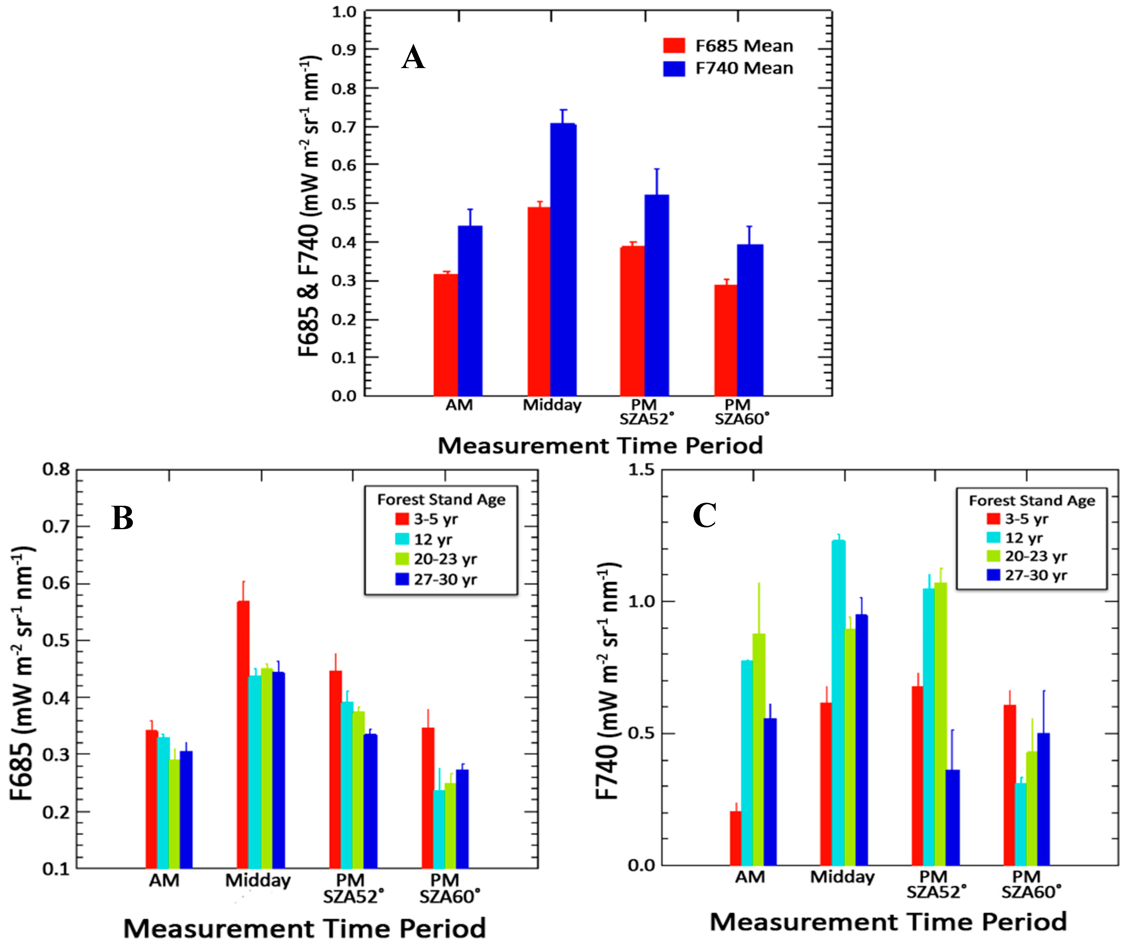
4.4. Far-Red vs. Red Fluorescence Radiances

In this coniferous forest during early fall senescence, the far-red fluorescence could not be shown to be correlated with any examined reflectance or structure variable across age groups, except for a weak association to one of the LiDAR-derived 3-D structure parameters, the vertical distribution ratio (VDR) for the open canopies of younger canopies (<12 year). Most surprising, the F740 was not well related to canopy GEP in this study, which is not consistent with results from several field investigations which have found significant positive correlations between F740 and canopy GEP [36,50,55,56]. One explanation may be that most of those studies were conducted during highly productive mid-season growing periods, when canopy TChl was high, and other foliar biochemical constituents and processes were in near-optimal conditions. One of the consequences of the variable fluorescence responses at different times of day and stand age classes is that an assumption that F685 (radiances or yields) can be predicted if F740 radiances (or yields) is known, as is assumed in some modeling approaches, is not supported by these campaign results (Figure 8, Figure 9 and Figure 10). Another explanation could be that stray light was only partially corrected for F740, increasing noise in the far red spectrum. Nevertheless, the F740 was extremely useful in this study because it provided a means to normalize the F685 so that the red/far-red Fratio (F685/F740) successfully described LUE in the mature LP stand.
The importance and success of the red fluorescence variables, as compared to the far-red fluorescence, is supported by several published radiative transfer modeling efforts and current state-of-the-art fluorescence models [57,58,59,60,61,62]. These papers demonstrate that the red fluorescence is more sensitive to vegetation physiological variables than the far-red fluorescence and is potentially retrievable from satellite orbit [63]. Retrieval of red fluorescence from satellite was recently reported [64], however, all other satellite fluorescence retrievals have been for the far-red fluorescence. These have all been acquired from coarse spatial resolution satellite observations obtained with atmospheric chemistry missions [14,65,66,67,68,69,70].

4.5. LiDAR Variables

When this campaign was designed, it was anticipated that LiDAR data would be important for sorting out the joint influences on fluorescence of forest canopy structure and canopy functionality. This expectation was realized, since the CHM structure parameter for canopy height derived from LiDAR returns was strongly related to LP stand age (r2 = 0.95, 2–33 years old in 2013), and was non-linearly related to F685 radiances (Figure 8). That particular finding was further studied in a separate analysis reported from this campaign [34] that capitalized on the inherent design of this site, based on the chronosequence of age classes. That study attributed the decline in F685 radiances and F685 yields across LP age classes to developmental processes that reduce hydraulic conductance in older trees [71,72], which would certainly affect the physiological performance we identified.

5. Conclusions

This study demonstrates the importance of diurnal observations for interpretation of fluorescence dynamics, as well as the utility of the red fluorescence for understanding canopy physiological processes, especially since red fluorescence responses were strongly affected by diurnal temperature differences and Loblolly pine stand age. The benefit of simultaneously acquiring fluorescence, high spectral resolution full-spectrum reflectance, and LiDAR observations from aircraft was demonstrated for describing vegetation structure, biochemical constituents, and physiological stress responses to the environmental conditions, at ecologically relevant (15–50 m) spatial scales during early fall senescence. In particular, the combination of the red fluorescence, the red/far-red Fratio, and the PRI together provide insight about canopy diurnal physiological dynamics, especially those driven by the canopy light regime and temperature. The Fratio obtained for the mature Loblolly pine stand at the NC2 tower site was strongly related to canopy LUE. The difficulty of estimating canopy carbon uptake using remote sensing acquisitions obtained at/around solar noon when both the spectral and flux data were nearly constant, versus measurements acquired under changing mid-morning and afternoon time periods, was demonstrated. We note that whereas the combination of LiDAR CHM with VSWIR spectra provided the optimal LP stand age class map, the VSWIR spectra alone discriminated these age classes quite well. This is useful information for the future FLEX satellite, which in tandem with Sentinel-3 will collect wavelengths (but not continuous spectra) across the VSWIR spectrum. This capability could be ensured if FLEX and the NASA HypIRI mission, which will collect VSWIR spectra, were flown during the same years. We note that our study reveals the importance of quantifying the diurnal fluorescence dynamics related to irradiance and thermal influences on canopy physiology, which will likely be addressed through modeling of these responses. However, much more needs to be learned about the diurnal expression of these responses, including variability across plant types, and their expression throughout the annual cycle.
We recommend that additional airborne campaigns utilizing a similar suite of instruments be conducted during summertime at peak production and throughout the growing season over other well-characterized study sites, especially fruitful when paired with a flux tower, to complement and reinforce the findings of this unique experiment conducted during fall senescence in a managed pine forest.

Acknowledgments

Funding for FLEX-US 2013 was provided by the European Space Agency (ESA Contract No. 4000109199/13/NL/FF/lf), NASA HQ (J. Kaye), and NASA/GSFC (Code 610). The development of HyPlant was supported by the large scale investment grant of the Forschungszentrum Jülich, Germany. Further support for campaign activities was provided by the SFB/TR 32 “Patterns in Soil-Vegetation-Atmosphere Systems: Monitoring, Modelling, and Data Assimilation”—subproject D2 (www.tr32.de), funded by the Deutsche Forschungsgemeinschaft (DFG), Germany. The work at the Parker Tract, NC (US-NC2) site was supported by USDA Forest Service Eastern Forest Environmental Threat Assessment Center Cooperative Agreements 03-CA-11330147-073 and 04-CA-11330147-238, DOE-National Institute for Climate Change Research (NICCR) Award 08-SC-NICCR-1072, Department of the Interior (DOI) Southeast Climate Science Center Award G10AC00624, DOE Terrestrial Ecosystem Science Award 11-DE-SC-0006700, and USDA NIFA Awards 2011-68002-30185 and 2014-67003-22068. The FLEX-US team gratefully acknowledges the roles of Ge Sun (USDA Forest Service (FS), Eastern Forest Environmental Threat Assessment Center, Raleigh, NC, USA) and Steve McNulty (USDA Forest Service, South-Eastern Regional Climate Hub, Raleigh, NC, USA) in providing funding and other support of the US-NC2 site, including ancillary modeling research. We also thank Drs. Sergio Cogliati and Tommaso Julitta (Dept. Environ. Sciences, U. Milano-Bicocca, Milano, Italy) for their contributions to this project. We also acknowledge the assistance of Susan Huemmrich for field support; the GSFC Aerosol Robotic Network (AERONET) program for lending instrumentation and expertise on atmospheric characterization; VA Tech (Blacksburg, VA, USA) students Beth Stein and Katie Britt; the staff of the Vernon G. James Research and Extension Center (managed by NC Dept. of Agriculture and NC State; and the staff at NASA/LaRC for airborne support.

Author Contributions

The campaign was co-led by E. Middleton and U. Rascher, with ESA management provided by R. Bianchi and D. Schuettemeyer. The airborne flights were conducted by B.D. Cook, L.A. Corp, and A. Schickling. Ground calibration/validation data were collected by K.F. Huemmrich and Q. Zhang. Flux tower data were processed by A. Noormets and provided in graphical form by K.F. Huemmrich. HyPlant data processing was managed by U. Rascher, with data processing undertaken by F. Pinto, L. Alonso, A. Damm, and L. Guanter. G-LiHT data were processed by L.A. Corp and B.D. Cook. HyPlant and G-LiHT data were combined for analysis by L.A. Corp. Partial data evaluations were conducted by R. Colombo, M. Rossini, and P.K.E. Campbell. Statistical analyses and manuscript writing were performed by E.M. Middleton. Graphics and manuscript support was provided by D.R. Landis.

Conflicts of Interest

The authors declare no conflict of interest.

Abbreviations

AOI or ROIspatial Area Of Interest or Region Of Interest
ASLAbove Sea Level
CHMCanopy Height Model
CCDCharge-Coupled Device
DBHDiameter was measured at Breast Height
DNDigital Number
DTMDigital Terrain Model
EGM96Earth Gravitational Model 1996
FOVField Of View
FLEXFLuorescence EXplorer
FLEX-USCollaborative ESA/FLEX and NASA/GSFC airborne campaign in the USA
GEPGross Ecosystem Production
G-LiHTGoddard’s Lidar, Hyperspectral, and Thermal airborne system
GSFCNASA Goddard Space Flight Center
GPPGross Primary Production
GPSGeographic Positioning System
HyspIRIHyperspectral InfraRed Imager
INSInertial Navigation System
LAILeaf Area Index
LaRCNASA Langley Research Center
LiDARLight Detection And Ranging
LPLoblolly Pine
LUELight Use Efficiency
LWIRLongWave InfraRed
MERISMedium Resolution Imaging Spectrometer
MIRMiddle InfraRed
MTCIMERIS Terrestrial Chlorophyll Index
NCNorth Carolina (USA)
NDVINormalized Difference Vegetation Index
NEPNet Ecosystem Production and ecosystem respiration
NIRNear InfraRed
NISTUS National Institute of Standards and Technology
NETDNoise Equivalent Temperature Difference
PARiincident Photosynthetically Active Radiation
PRIPhotochemical Reflectance Index
RGBRed Green Blue
ROIRegion Of Interest
SEMStandard Error of the Mean
SDStandard Deviation
SIFSolar-Induced chlorophyll Fluorescence
SNRSignal to Noise Ratio
SVSingular Vector
SVDSingular Vector Decomposition method
SWIRShortWave InfraRed
SZASolar Zenith Angle
TChlTotal canopy Chlorophyll
TINTriangulated Irregular Network
VDRVertical Distribution Ratio (VDR)
VNIRVisible to Near InfraRed
VSWIRVisible to ShortWave InfraRed

References

  1. Drusch, M.; Moreno, J.; del Bello, U.; Franco, R.; Goulas, Y.; Huth, A.; Kraft, S.; Middleton, E.; Miglietta, F.; Mohammad, G.; et al. The Fluorescence EXplorer (FLEX) Mission Concept—ESA’s Earth Explorer 8 (EE8). IEEE Trans. Geosci. Remote Sens. 2017, 55, 1273–1284. [Google Scholar] [CrossRef]
  2. European Space Agency (ESA). Report for Mission Selection; FLEX, ESA SP-1330/2 (2 Volume Series); European Space Agency: Noordwijk, The Netherlands, 2015. [Google Scholar]
  3. Rascher, U.; Alonso, L.; Burkart, A.; Cilia, C.; Cogliati, S.; Colombo, R.; Damm, A.; Drusch, M.; Guanter, L.; Hanus, J.; et al. Sun-induced fluorescence—A new probe of photosynthesis: First maps from the imaging spectrometer HyPlant. Glob. Chang. Biol. 2015, 21, 4673–4684. [Google Scholar] [CrossRef] [PubMed]
  4. Cook, B.D.; Corp, L.A.; Nelson, R.F.; Middleton, E.M.; Morton, D.C.; McCorkel, J.T.; Masek, J.G.; Ranson, K.J.; Ly, V.; Montesano, P.M. NASA Goddard’s Lidar, Hyperspectral and Thermal (G-LiHT) airborne imager. Remote Sens. 2013, 5, 4045–4066. [Google Scholar] [CrossRef]
  5. Corp, L.; Middleton, E.; Cook, B.; Campbell, P.; Huemmrich, F.; Rasher, U.; Pinto, F. Airborne Remote Sensing to Define Ecosystem Form & Function over a Loblolly Pine Plantation. In Proceedings of the International Geoscience and Remote Sensing Symposium (IGARSS15), Milan, Italy, 26–31 July 2015. [Google Scholar]
  6. Corp, L.A.; Cook, B.D.; McCorkel, J.; Middleton, E.M. Data products of NASA Goddard’s LiDAR, Hyperspectral, and Thermal Airborne Imager (G-LiHT). In Proceedings of the SPIE DSS Defense, Security, and Sensing Symposium, Baltimore, MD, USA, 20–24 April 2015; p. 12. [Google Scholar]
  7. Forschungszentrum. FLEX-US Final Report, Technical Assistance for the Deployment of the Airborne HyPlant Imaging Spectrometer during 2013 ESA/NASA Joint FLEX-US (FLuorescence EXplorer Experiment in USA) Ampaign; Forschungszentrum: Jülich, Germany, 2015. [Google Scholar]
  8. Noormets, A.; McNulty, S.G.; Gavazzi, M.J.; Sun, G.; Domec, J.C.; King, J.; Chen, J. Response of carbon fluxes to drought in a coastal plain loblolly pine forest. Glob. Chang. Biol. 2009, 16, 272–287. [Google Scholar] [CrossRef]
  9. Noormets, A.; McNulty, S.G.; Domec, J.C.; Gavazzi, M.; Sun, G.; King, J.S. The role of harvest residue in rotation cycle carbon balance in loblolly pine plantations. Respiration partitioning approach. Glob. Chang. Biol. 2012, 18, 3186–3201. [Google Scholar] [CrossRef]
  10. Rossini, M.; Nedbal, L.; Guanter, L.; Ač, A.; Alonso, L.; Burkart, A.; Cogliati, S.; Colombo, R.; Damm, A.; Drusch, M.; et al. Red and far red Sun-induced chlorophyll fluorescence as a measure of plant photosynthesis. Geophys. Res. Lett. 2015, 42, 1632–1639. [Google Scholar] [CrossRef]
  11. G-LiHT Web Site. Available online: http://gliht.gsfc.nasa.gov/ (accessed on 4 May 2017).
  12. G-LiHT White Paper. Available online: https://gliht.gsfc.nasa.gov/specs/ (accessed on 4 May 2017).
  13. Goulden, M.L.; Winston, G.C.; McMillan, A.; Litvak, M.E.; Read, E.L.; Rocha, A.V.; Elliot, J.R. An eddy covariance mesonet to measure the effect of forest age on land–atmosphere exchange. Glob. Chang. Biol. 2006, 12, 2146–2162. [Google Scholar] [CrossRef]
  14. Guanter, L.; Frankenberg, C.; Dudhia, A.; Lewis, P.E.; Gómez-Dans, J.; Kuze, A.; Suto, H.; Grainger, R.G. Retrieval and global assessment of terrestrial chlorophyll fluorescence from GOSAT space measurements. Remote Sens. Environ. 2012, 121, 236–251. [Google Scholar] [CrossRef]
  15. Guanter, L.; Rossini, M.; Colombo, R.; Meroni, M.; Frankenberg, C.; Lee, J.-E.; Joiner, J. Using field spectroscopy to assess the potential of statistical approaches for the retrieval of sun-induced chlorophyll fluorescence from space. Remote Sens. Environ. 2013, 133, 52–61. [Google Scholar] [CrossRef]
  16. Berk, A.; Conforti, P.; Hawes, F. An accelerated line-by-line option for MODTRAN combining on-the-fly generation of line center absorption with 0.1 cm−1 bins and pre-computed line tails, 21 May 2015. Proc. SPIE 2015. [Google Scholar] [CrossRef]
  17. Berk, A.; Conforti, P.; Kennett, R.; Perkins, T.; Hawes, F.; van den Bosch, J. MODTRAN6: A major upgrade of the MODTRAN radiative transfer code, 13 June 2014. Proc. SPIE 2014. [Google Scholar] [CrossRef]
  18. Richter, R.; Schläpfer, D. Atmospheric/Topographic Correction for Airborne Imagery; DLR Report DLR-IB 565-02/15; DLR: Wessling, Germany, 2015; p. 254. [Google Scholar]
  19. Schläpfer, D.; Richter, R.; Feingersh, T. Operational BRDF Effects Correction for Wide-Field-of-View Optical Scanners (BREFCOR). IEEE TGARS 2015, 53, 1855–1864. [Google Scholar] [CrossRef]
  20. G-LiHT List of Plot Scale Metrics. Available online: ftp://fusionftp.gsfc.nasa.gov/multimedia/docs/metrics_readme.pdf (accessed on 4 May 2017).
  21. Lee, C.M.; Cable, M.L.; Hook, S.J.; Green, R.O.; Ustin, S.L.; Mandl, D.J.; Middleton, E.M. An introduction to the NASA Hyperspectral InfraRed Imager (HyspIRI) mission and preparatory activities. Special Issue on HyspIRI. Remote Sens. Environ. 2015, 167, 6–19. [Google Scholar] [CrossRef]
  22. Gamon, J.A.; Peñuelas, J.; Field, C.B. A narrow-wavelength spectral index that tracks diurnal changes in photosynthetic efficiency. Remote Sens. Environ. 1992, 41, 35–44. [Google Scholar] [CrossRef]
  23. Gamon, J.A.; Serrano, L.; Surfus, J.S. The photochemical reflectance index: An optical indicator of photosynthetic radiation use efficiency across species, functional types, and nutrient levels. Oecologia 1997, 112, 492–501. [Google Scholar] [CrossRef] [PubMed]
  24. Filella, I.; Amaro, T.; Araua, J.L.; Peñuelas, J. Relationship between photosynthetic radiation-use efficiency of barley canopies and the photochemical reflectance index (PRI). Physiol. Plant. 1996, 96, 211–216. [Google Scholar] [CrossRef]
  25. Rouse, J.W.; Haas, R.H.; Scheel, J.A.; Deering, D.W. Monitoring vegetation systems in the Great Plains with ERTS. In Proceedings of the 3rd Earth Resource Technology Satellite (ERTS) Symposium, Washington, DC, USA, 10–14 December 1973. [Google Scholar]
  26. Tucker, C.J. Red and Photographic Infrared Linear Combinations for Monitoring Vegetation. Remote Sens. Environ. 1979, 8, 127–150. [Google Scholar] [CrossRef]
  27. Dash, J.; Curran, P.J. Evaluation of the MERIS terrestrial chlorophyll index (MTCI). Adv. Space Res. 2007, 9, 100–104. [Google Scholar] [CrossRef]
  28. Dash, J.; Curran, P.J.; Tallis, M.J.; Llewellyn, G.M.; Taylor, G.; Snoeij, P. Validating the MERIS Terrestrial Chlorophyll Index (MTCI) with ground chlorophyll content data at MERIS spatial resolution. Int. J. Remote Sens. 2010, 31, 5513–5532. [Google Scholar] [CrossRef]
  29. Lichtenthaler, H.K.; Rinderle, U. The role of chlorophyll fluorescence in the detection of stress conditions in plants. CRC Crit. Rev. Anal. Chem. 1988, 19, S29–S85. [Google Scholar] [CrossRef]
  30. Agati, G.; Mazzinghi, P.; Fusi, F.; Ambrosini, I. The F685/F730 chlorophyll fluorescence ratio as a tool in plant physiology: Response tophysiological and environmental factors. J. Plant Physiol. 1995, 145, 228–238. [Google Scholar] [CrossRef]
  31. Porcar-Castell, A.; Tyystjärvi, E.; Atherton, J.; van der Tol, C.; Flexas, J.; Pfündel, E.E.; Moreno, J.; Frankenberg, C.; Berry, J.A. Linking chlorophyll a fluorescence to photosynthesis for remote sensing applications: Mechanisms and challenges. J. Exp. Bot. 2014, 65, 4065–4095. [Google Scholar] [CrossRef] [PubMed]
  32. Cheng, Y.-B.; Middleton, E.M.; Zhang, Q.; Huemmrich, K.F.; Campbell, P.K.; Corp, L.A.; Cook, B.D.; Kustas, W.P.; Daughtry, C.S. Integrating Solar Induced Fluorescence and the Photochemical Reflectance Index for Estimating Gross Primary Production in a Cornfield. Remote Sens. 2013, 5, 6857–6879. [Google Scholar] [CrossRef]
  33. Rossini, M.; Meroni, M.; Celesti, M.; Cogliati, S.; Julitta, T.; Panigada, C.; Rascher, U.; van der Tol, C.; Colombo, R. Analysis of Red and Far-Red Sun-Induced Chlorophyll Fluorescence and Their Ratio in Different Canopies Based on Observed and Modeled Data. Remote Sens. 2016, 8, 412. [Google Scholar] [CrossRef]
  34. Colombo, R.; Celesti, M.; Campbell, P.; Cogliati, S.; Cook, B.; Corp, L.A.; Damm, A.; Guanter, L.; Julitta, T.; Middleton, E.M.; et al. On the variability of sun-induced chlorophyll fluorescence according stand age related processes in a loblolly pine forest. Remote Sens. Environ. 2017. in review. [Google Scholar]
  35. Middleton, E.M.; Cheng, Y.-B.; Campbell, P.E.; Huemmrich, K.F.; Corp, L.A.; Bernardes, S.; Zhang, Q.; Landis, D.R.; Kustas, W.P.; Daughtry, C.S.T.; et al. Multi-angle hyperspectral observations with SIF and PRI to detect plant stress & GPP in a cornfield. In Proceedings of the 9th EARSeL SIG Workshop on Imaging Spectroscopy, CD-ROM, Luxembourg, 14–16 April 2015; p. 10. [Google Scholar]
  36. Rascher, U.; Schickling, A.; Damm, A.; Udelhoven, T. Canopy fluorescence improves modeling of diurnal courses of GPP-correlation of GPP and Fs over a variety of crops. In Proceedings of the 4th International Workshop on Remote Sensing of Vegetation Fluorescence, Valencia, Spain, 15–17 November 2010. [Google Scholar]
  37. Barton, C.V.M.; North, P.R.J. Remote sensing of canopy light use efficiency using the photochemical reflectance index: Model and sensitivity analysis. Remote Sens. Environ. 2001, 78, 264–273. [Google Scholar] [CrossRef]
  38. Garbulsky, M.F.; Peñuelas, J.; Gamon, J.; Inoue, Y.; Filella, I. The photochemical reflectance index (PRI) and the remote sensing of leaf, canopy and ecosystem radiation use efficiencies: A review and meta-analysis. Remote Sens. Environ. 2011, 115, 281–297. [Google Scholar] [CrossRef]
  39. Middleton, E.M.; Cheng, Y.-B.; Hilker, T.; Black, T.A.; Krishnan, P.; Coops, N.C.; Huemmrich, K.F. Linking foliage spectral responses to canopy level ecosystem photosynthetic light use efficiency at a Douglas-fir forest in Canada. Can. J. Remote Sens. 2009, 35, 166–188. [Google Scholar] [CrossRef]
  40. Peñuelas, J.; Garbulsky, M.F.; Filella, I. Photochemical reflectance index (PRI) and remote sensing of plant CO2 uptake. New Phytol. 2011, 191, 596–599. [Google Scholar] [CrossRef]
  41. Filella, I.; Porcar-Castell, A.; Munné-Bosch, S.; Bäck, J.; Garbulsky, M.G.; Peñuelas, J. PRI assessment of long-term changes in carotenoids/chlorophyll ratio and short-term changes in de-epoxidation state of the xanthophyll cycle. Int. J. Remote Sens. 2009, 30, 4443–4455. [Google Scholar] [CrossRef]
  42. Gamon, J.A.; Huemmrich, K.F.; Wong, C.Y.S.; Ensminger, I.; Garrity, S.; Hollinger, D.Y.; Noormets, A.; Peñuelas, J. A remotely sensed pigment index reveals photosynthetic phenology in evergreen conifers. Proc. Natl. Acad. Sci. USA 2016, 113, 13087–13092. [Google Scholar] [CrossRef] [PubMed]
  43. Garrity, S.R.; Eitel, J.U.H.; Vierling, L.A. Disentangling the relationships between plant pigments and the photochemical reflectance index reveals a new approach for remote estimation of carotenoid content. Remote Sens. Environ. 2011, 115, 628–635. [Google Scholar] [CrossRef]
  44. Stylinski, C.D.; Gamon, J.A.; Oechel, W.C. Seasonal patterns of reflectance indices, carotenoid pigments and photosynthesis of evergreen chaparral species. Oecologia 2002, 131, 366–374. [Google Scholar] [CrossRef] [PubMed]
  45. Zarco-Tejada, P.J.; González-Dugo, V.; Berni, J.A. Fluorescence, temperature and narrow-band indices acquired from a UAV platform for water stress detection using a micro-hyperspectral imager and a thermal camera. Remote Sens. Environ. 2012, 117, 322–337. [Google Scholar] [CrossRef]
  46. Zarco-Tejada, P.J.; González-Dugo, V.; Williams, L.E.; Suárez, L.; Berni, J.A.; Goldhamer, D.; Fereres, E. A PRI-based water stress index combining structural and chlorophyll effects: Assessment using diurnal narrow-band airborne imagery and the CWSI thermal index. Remote Sens. Environ. 2013, 138, 38–50. [Google Scholar] [CrossRef]
  47. Ac, A.; Malenovsky, Z.; Olejnickova, J.; Gallé, A.; Rascher, U.; Mohammed, G. Meta-analysis assessing potential of steady-state chlorophyll fluorescence for remote sensing detection of plant water, temperature and nitrogen stress. Remote Sens. Environ. 2015, 168, 420–436. [Google Scholar] [CrossRef]
  48. Middleton, E.M.; Huemmrich, K.F.; Cheng, Y.-B.; Margolis, H.A. Spectral bio-indicators of photosynthetic efficiency and vegetation stress. In Hyperspectral Remote Sensing of Vegetation; Thenkabail, P.S., Lyon, J.G., Huete, A., Eds.; Taylor & Francis: Abingdon-on-Thames, UK, 2012. [Google Scholar]
  49. Middleton, E.M.; Cheng, Y.-B.; Campbell, P.E.; Huemmrich, K.F.; Zhang, Q.; Landis, D.R.; Kustas, W.P.; Daughtry, C.S.T.; Russ, A.L. Directional Hyperspectral Observations to Detect Plant Stress with the PRI and SIF in a Cornfield. In Proceedings of the 4th Recent Advances in Quantitative Remote Sensing (RAQRS’IV), Valencia, Spain, 22–26 September 2014. [Google Scholar]
  50. Meroni, M.; Rossini, M.; Picchi, V.; Panigada, C.; Cogliati, S.; Nali, C.; Colombo, R. Assessing Steady-state Fluorescence and PRI from Hyperspectral Proximal Sensing as Early Indicators of Plant Stress: The Case of Ozone Exposure. Sensors 2008, 8, 1740–1754. [Google Scholar] [CrossRef] [PubMed]
  51. Middleton, E.; Cheng, Y.; Corp, L.; Huemmrich, K.; Campbell, P.; Zhang, Q.-Y.; Kustas, W.; Russ, A. Diurnal and seasonal dynamics of canopy-level solar-induced chlorophyll fluorescence and spectral reflectance indices in a cornfield. In Proceedings of the 6th EARSeL SIG Workshop on Imaging Spectroscopy, CD-ROM, Tel-Aviv, Israel, 16–19 March 2009. [Google Scholar]
  52. Schickling, A.; Matveeva, M.; Damm, A.; Schween, J.H.; Wahner, A.; Graf, A.; Crewell, S.; Rascher, U. Combining sun-induced chlorophyll fluorescence and Photochemical Reflectance Index improves diurnal modeling of gross primary productivity. Remote Sens. 2016, 8, 574. [Google Scholar] [CrossRef]
  53. Middleton, E.M.; Huemmrich, K.F.; Landis, D.R.; Black, T.A.; Barr, A.; McCaughey, J.H. Remote sensing of ecosystem light use efficiency using MODIS. Remote Sens. Environ. 2016, 187, 345–366. [Google Scholar] [CrossRef]
  54. Wieneke, S.; Ahrends, H.; Damm, A.; Pinto, F.; Stadler, A.; Rossini, M.; Rascher, U. Airborne based spectroscopy of red and far-red sun-induced chlorophyll fluorescence: Implications for improved estimates of gross primary productivity. Remote Sens. Environ. 2016, 184, 654–667. [Google Scholar] [CrossRef]
  55. Damm, A.; Elbers, J.; Erler, A.; Gioli, B.; Hamdi, K.; Hutjes, R.; Kosvancova, M.; Meroni, M.; Miglietta, F.; Moersch, A.; et al. Remote sensing of sun-induced fluorescence to improve modeling of diurnal courses of gross primary production (GPP). Glob. Chang. Biol. 2010, 16, 171–186. [Google Scholar] [CrossRef]
  56. Damm, A.; Guanter, L.; Paul-Limoges, E.; van der Tol, C.; Hueni, A.; Buchmann, N.; Eugster, W.; Ammann, C.; Schaepman, M.E. Far-red sun-induced chlorophyll fluorescence shows ecosystem-specific relationships to gross primary production: An assessment based on observational and modeling approaches. Remote Sens. Environ. 2015, 166, 91–105. [Google Scholar] [CrossRef]
  57. Cheng, Y.-B.; Zhang, Q.; Lyapustin, A.I.; Wang, Y.; Middleton, E.M. Impacts of light use efficiency and fPAR parameterization on gross primary production modeling. Agric. For. Meteorol. 2014, 189–190, 187–197. [Google Scholar] [CrossRef]
  58. Damm, A.; Guanter, L.; Verhoef, W.; Schläpfer, D.; Garbari, S.; Schaepman, M.E. Impact of varying irradiance on vegetation indices and chlorophyll fluorescence derived from spectroscopy data. Remote Sens. Environ. 2015, 156, 202–215. [Google Scholar] [CrossRef]
  59. Van der Tol, C.; Verhoef, W.; Timmermans, J.; Verhoef, A.; Su, Z. An integrated model of soil-canopy spectral radiances, photosynthesis, fluorescence, temperature and energy balance. Biogeosciences 2009, 6, 3109–3129. [Google Scholar] [CrossRef]
  60. Vilfan, N.; Van der Tol, C.; Müller, O.; Rascher, U.; Verhoef, W. Fluspect-B: A model for fluorescence, reflectance and transmittance spectra. Remote Sens. Environ. 2016, 86, 596–615. [Google Scholar] [CrossRef]
  61. Cogliati, S.; Verhoef, W.; Kraft, S.; Sabater, N.; Alonso, L.; Vicent, J.; Moreno, J.; Drusch, M.; Colombo, R. Retrieval of sun-induced fluorescence using advanced spectral fitting methods. Remote Sens. Environ. 2015, 169, 344–357. [Google Scholar] [CrossRef]
  62. Verrelst, J.; van der Tol, C.; Magnani, F.; Sabater, N.; Rivera, J.P.; Mohammed, G.; Moreno, J. Evaluating the predictive power of sun-induced chlorophyll fluorescence to estimate net photosynthesis of vegetation canopies: A SCOPE modeling study. Remote Sens. Environ. 2016, 176, 139–151. [Google Scholar] [CrossRef]
  63. Verhoef, W.; van der Tol, C.; Middleton, E.M. Hyperspectral radiative transfer modeling to explore the combined retrieval of biophysical parameters and canopy fluorescence from FLEX—Sentinel-3 tandem mission multi-sensor data. Remote Sens. Environ. 2017. in review 2017. [Google Scholar]
  64. Joiner, J.; Yoshida, Y.; Guanter, L.; Middleton, E.M. New methods for retrieval of chlorophyll red fluorescence from hyperspectral satellite instruments: Simulations and application to GOME-2 and SCIAMACHY. Atmos. Meas. Tech. 2016, 9, 3939–3967. [Google Scholar] [CrossRef]
  65. Joiner, J.; Yoshida, Y.; Vasilkov, A.P.; Yoshida, Y.; Corp, L.A.; Middleton, E.M. First observations of global and seasonal terrestrial chlorophyll fluorescence from space. Biogeosciences 2011, 8, 637–651. [Google Scholar] [CrossRef]
  66. Joiner, J.; Yoshida, Y.; Vasilkov, A.P.; Middleton, E.M.; Campbell, P.K.E.; Kuze, A.; Corp, L.A. Filling-in of near-infrared solar lines by terrestrial fluorescence and other geophysical effects: Simulations and space-based observations from SCIAMACHY and GOSAT. Atmos. Meas. Tech. 2012, 5, 809–829. [Google Scholar] [CrossRef]
  67. Joiner, J.; Guanter, L.; Lindstrot, R.; Voigt, M.; Vasilkov, A.P.; Middleton, E.M.; Huemmrich, K.F.; Yoshida, Y.; Frankenberg, C. Global monitoring of terrestrial chlorophyll fluorescence from moderate-spectral-resolution near-infrared satellite measurements: Methodology, simulations, and application to GOME-2. Atmos. Meas. Tech. 2013, 6, 2803–2823. [Google Scholar] [CrossRef]
  68. Guanter, L.; Zhang, Y.G.; Jung, M.; Joiner, J.; Voigt, M.; Berry, J.A.; Frankenberg, C.; Huete, A.R.; Zarco-Tejada, P.; Lee, J.-E.; et al. Global and time-resolved monitoring of crop photosynthesis with chlorophyll fluorescence. Proc. Natl. Acad. Sci. USA 2014, 111, E1327–E1333. [Google Scholar] [CrossRef] [PubMed]
  69. Frankenberg, C.; Fisher, J.B.; Worden, J.; Badgley, G.; Saatchi, S.S.; Lee, J.-E.; Toon, G.C.; Butz, A.; Jung, M.; Kuze, A.; et al. New global observations of the terrestrial carbon cycle from GOSAT: Patterns of plant fluorescence with gross primary productivity. Geophys. Res. Lett. 2011, 38, L17706. [Google Scholar] [CrossRef]
  70. Frankenberg, C.; O’Dell, C.; Guanter, L.; McDuffie, J. Remote sensing of near-infrared chlorophyll fluorescence from space in scattering atmospheres: Implications for its retrieval and interferences with atmospheric CO2 retrievals. Atmos. Meas. Tech. 2012, 5, 2081–2094. [Google Scholar] [CrossRef]
  71. Domec, J.C.; Sun, G.; Noormets, A.; Gavazzi, M.J.; Treasure, E.A.; Cohen, E.; Swenson, J.J.; McNulty, S.G.; King, J.S. A comparison of three methods to estimate evapotranspiration in two contrasting loblolly pine plantations: Age-related changes in water use and drought sensitivity of evapotranspiration components. For. Sci. 2012, 58, 497–512. [Google Scholar] [CrossRef]
  72. Zaehle, S.; Sitch, S.; Prentice, C.; Liski, J.; Cramer, W.; Erhard, M.; Hickler, T.; Smith, B. The importance of age-related decline in forest NPP for modeling regional carbon balances. Ecol. Appl. 2006, 16, 1555–1574. [Google Scholar] [CrossRef]
Figure 1. The full Parker Tract NC loblolly pine plantation (near Plymouth, NC) is outlined in black on a Google Earth image. The white circle is the NC2 eddy covariance flux tower. The flight lines for this study: red lines are the fixed, parallel North-South mapping lines that were repeated for each of the four time period collections and used to produce the study area mosaic; yellow lines are the varying lines flown along the solar principal plane associated with the start and end of each collection which occurred at different times of day, and which were aligned to pass over the tower.
Remotesensing 09 00612 g001
Figure 2. The flight campaigns were initiated at the Langley Research Center in Hampton Roads, VA, using a King Air aircraft, the aft section of which is shown with some of the team members, (Left) left to right: Uwe Rascher, Roberto Colombo, Remo Bianchi, Petya Campbell, Larry Corp, Fred Huemmrich, Micol Rossini, Anke Schickling, Betsy Middleton, and Bruce Cook; (Right) A view of the two instrument packages inside the King Air, G-LiHT (forward) and HyPlant (aft).
Remotesensing 09 00612 g002
Figure 3. NC2 flux tower data at Parker Tract throughout 2013 (A,C,E) and October 2013 (B,D,F). GEP (µmol CO2 m−2 s−1): (A) average daily values throughout 2013; and (B) half hour values for the six days that include the campaign days. Incident PAR (µmol PARi m−2 s−1): (C) average daily values throughout 2013; and (D) for half hour values for six days that include the two campaign days, 26 October 2013. Light Use Efficiency, LUE (µmol CO2 µmol−1 photons): (E) the daily averages throughout 2013; and (F) half hour values for the six days that included the campaign days.
Remotesensing 09 00612 g003
Figure 4. Various G-LiHT LiDAR data products. (A) CHM data for 120 m × 120 m ROIs for 3 height categories within the Parker Tract study area (LP low, LP Med, LP High at NC2 Tower); (B) Bar chart describing the mean CHM ± SD (and minimum, maximum values) for the three height categories (n = 30 ROI); (C) Side View of a LiDAR Geo-referenced Point Cloud collected at 2 m, where first returns from tree crowns were processed through the CHM (yellow layer); the ground-level returns (blue layer) were determined with a Digital Terrain Model, DTM. The top of the flux tower is seen in the background; (D) 3-D site mosaic produced with CHM data overlaid on a G-LiHT RGB reflectance image from the VNIR spectrometer, which accentuates the variation in canopy heights across the site. The middle and bottom examples are from Duke Forest, NC.
Remotesensing 09 00612 g004
Figure 5. Thermal calibration of the G-LiHT thermal sensor against ground-based measurements.
Remotesensing 09 00612 g005
Figure 6. Map Products aggregated to 14 m partial resolution derived from mosaics of the parallel N-S flight lines (red lines, Figure 1) for the Parker Tract forest collected near solar noon on 26 October 2013. G-LiHT products: (A) true color RGB image derived from the G-LiHT VNIR imaging spectrometer (the numbers are the stand ages in years, as of 2013); (B) CHM from G-LiHT LiDAR observations for all vegetated areas (0–35 m); (C) the PRI hyperspectral reflectance index (values between −0.1 and 0.03) from the G-LiHT VNIR spectrometer; (D) the NDVI reflectance index (values, 0.4–0.9) from the G-LiHT VNIR spectrometer; and (E) the adjusted surface temperature (5–20 °C) from the G-LiHT thermal sensor. Areas shown in black (e.g., (B,D)) are flat fallow fields. HyPlant products: (F) The red-band F685 emissions derived at 685 nm; (G) the far-red F740 emissions derived at 740 nm; and (H) the Red/Far-red fluorescence ratio (Fratio, F685/F740). Bar scales for each map are provided below the mosaics. The distance scale indicates the site area observed is ~2 km × 8 km. The tower site is indicated with a black and white circle.
Remotesensing 09 00612 g006
Figure 7. (A) Spectra from the HyPlant DUAL VSWIR spectrometer, as processed with the ATCOR-4 routine, describe ten LP stand age groups (LP 2 to LP 31 years.) and a mixed pine/deciduous forest group (brown spectrum), collected near noon on 26 October 2017. The young to mature LP stand ages are indicated by spectra of different colors: 2 year (purple), 3–4 year (navy, bright blue), intermediate age classes of 12, 14, 21, 23, and 27 year (dark-green, light-blue. aqua. bright-green, yellow), and the oldest age classes of 29 year (orange) and 31 year (red); (B) A forest classification map of the Parker Tract forest was obtained by merging the mosaics of these HyPlant DUAL VSWIR spectra with G-LiHT LiDAR CHM. Black areas indicate fallow fields.
Remotesensing 09 00612 g007
Figure 8. The canopy height and fluorescence information were obtained for the LP stands by age class, for ROIs (data aggregated to 49 m2) across the Parker Tract site: (A) F685 and F740 (mW m−2 sr−1 nm−1), derived from HyPlant’s FLUO module vs. stand age; (B) the Fratio, F685/F740 vs. stand age. Means and standard errors are shown for bar charts, N = 30 stands. Fluorescence values were averaged over all measurement collections per stand age group for the four time periods.
Remotesensing 09 00612 g008
Figure 9. The canopy solar-induced fluorescence emissions (means ± SE) acquired by the HyPlant FLUO at each of the four diurnal measurement periods (morning, mid-day, early afternoon, and mid-afternoon) acquired on 26 and 27 October are shown for: (A) fluorescence (W m−2 sr−1 nm−1) averaged over all stands (means ± SE) at each time period, for the red (F685, red bars) and far-red (F740, blue bars); (B) F685 for the four forest stand age groups (3–5 year (red); 12 year (aqua); 20–23 year (lime), and 27–30 year (navy)) within each of the four diurnal measurement periods; and (C) F740, same as (B).
Remotesensing 09 00612 g009
Figure 10. The canopy fluorescence yields (F/PARi, means ± SE, J umol−1 PAR sr−1 nm−1) and two pigment-related indices are shown for four forest stand age groups, at each of the four diurnal measurement periods: (A) the F685 yield; (B) the F740 yield; (C) the Fratio (F685/F740); (D) the MTCI estimate for relative TChl content; and (E) the PRI. The four age groups are: 3–5 year (age 1); 12 year (age 2); 20–23 year (age 3), and 27–30 year (age 4). Bar colors show responses per age group at the 4 diurnal collections: AM @ 60° SZA (red); mid-day @ 49° SZA (aqua); early afternoon @ 52° SZA (lime); and afternoon @ 60° SZA (navy).
Remotesensing 09 00612 g010
Figure 11. The relationships of the PRI to two canopy-scale spectral variables for the four age groups across all LP stands (ROIs, 49 m2): (A) TChl (MTCI) for the four age class groups produced an overall linear relationship (overall: r2 = 0.96, p ≤ 0.003, n = 143; age class, p ≤ 0.000); and (B) the F685 (r2 = 0.90, p ≤ 0.000, n = 138) with two age class groups. Age groups: 3–5 year (red circles), 12 year (aqua X), 21–23 year (lime +), and 27–31 year (navy triangles).
Remotesensing 09 00612 g011
Figure 12. The relationships of three canopy spectral indices to the relative canopy temperature (canopy-air, °C) at four times of day (n = 135): (A) the overall linear relationship for PRI vs. temperature difference (r = 0.98, p ≤ 0.000); (B) F685, tracking the fluorescence change per time period, showing an overall inverse response (r = 0.80) but different diurnal hysteresis temperature trends across the four time periods, for the two age groups (age 1, 2–12 year; age 2, 15–30 year), where the responses of the two age groups are indicated with the arrows and (C) the non-significant results for F740. The legends for (B) and (C) are the same.
Remotesensing 09 00612 g012
Figure 13. Fluxes at the NC2 eddy covariance tower in the mature LP stand (age class 4, 27–33 year): (A) the Fratio (F685/F740) vs. the photosynthetic light use efficiency (LUE, GPP/APARestimated, J µmol−1 PAR sr−1 nm−1) for two time groups, mid-day (red triangles) and morning/afternoon combined (blue circles); the relationships are linear, but depend on time of day (r2 = 0.84, p ≤ 0.000, F-ratio = 32.02, n = 31; p ≤ 0.000). Stronger results were obtained for the combined morning/afternoon set only, LUE (r = 0.96, SEM of 0.002), where, LUE = 0.016 + 0.027 × Fratio. (B) The influence of the temperature difference (canopy-air, °C) on canopy LUE varied throughout the day (r2 = 0.82, p ≤ 0.02, n = 47). (C) The measured GEP vs. the estimated GEP (µmol CO2 µmol−1 PAR) at three time periods. The estimated GEP was computed with three remote sensing variables: F685 yield, the PRI, and NDVI (r = 0.75).
Remotesensing 09 00612 g013
Figure 14. Hysteresis at four times over the diurnal cycle is expressed in the combined responses of F685 and the PRI: (A) the mature LP stand at the NC2 tower site; and (B) all ROI stands, including the NC2 tower stand.
Remotesensing 09 00612 g014
Figure 15. The AmeriFlux NC2 flux tower data at Parker Tract showing half hour flux values for six summer days, 13–19 June 2013. (A) GEP (µmol CO2 m−2 s−1); (B) Incident PAR (µmol PARi m−2 s−1); and (C) Light Use Efficiency, LUE (µmol CO2 µmol−1 photons).
Remotesensing 09 00612 g015
Table 1. Survey Measurements at the Parker Tract Site.
Measurements and Data CollectionsParker Tract, NC (Pinus taeda)
Site location (degrees latitude, longitude)35.8031, −76.6679
Mature Loblolly Site (US-NC2)Canopy function (Gross Ecosystem Production): AmeriFlux Eddy covariance tower
Multiple Stands
Field measurement datesContinuous, 23 September to 27 October 2013
Forest survey and GPS of measurementsVT, field guides/GPS
Vegetation heightVT, Clinometers
Leaf Area Index (LAI)VT, LAI-2000 Plant canopy analyzers
Tree diameter at breast height, DBHVT, Tree diameter at 1.30 m
Canopy (forest) densityVT, Within 1/10 acre plot, Prism
Stand ageVT, Field determination
VT—Students, Virginia Polytechnic Institute and State University (Blacksburg, Virginia).

