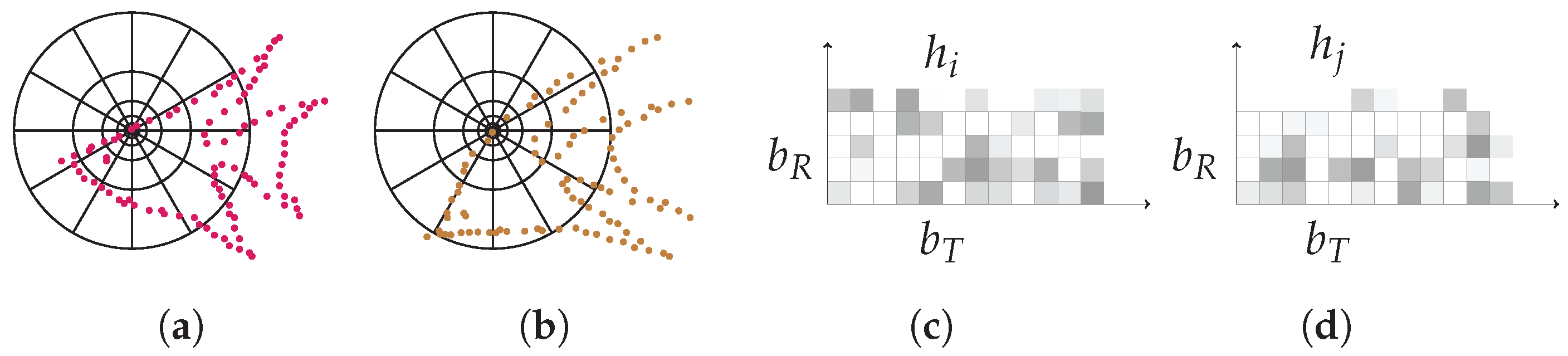
Figure 1.
Illustration of the SC. (a) and (b): diagrams of log-polar histogram bins centered at and used in computing the shape contexts. (c) and (d): each shape context e.g., or is a log-polar histogram of the coordinates of the rest of the point set measured using the centered point as the origin, where darker denotes larger value.
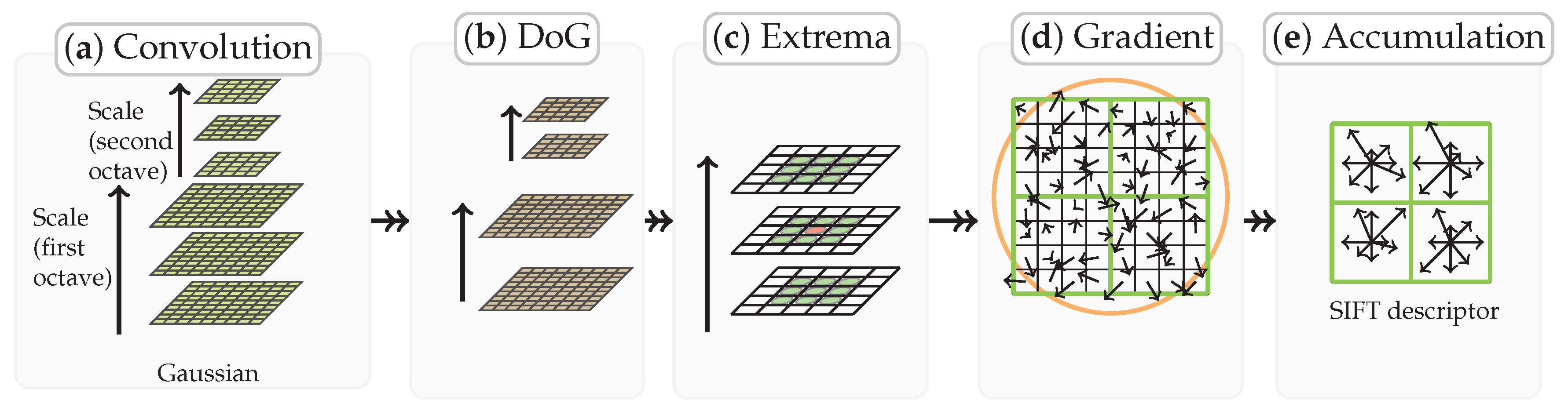
Figure 2.
Illustration of how the SIFT feature descriptor is obtained. (a): Repeatedly convolving initial image with Gaussians to produce the set of scale space images. (b): Subtracting adjacent Gaussian images to produce the difference-of-Gaussian images. (c): Extrema detection by comparing a pixel (marked with red circle) to its 26 neighbors in regions at the current and adjacent scales (marked with green circles). (d): Feature descriptor creation by computing the gradient magnitude and orientation at each image sample point. a Gaussian window indicated by the overlaid circle is used as weighting. (e) Orientation histograms accumulation by summarizing the contents over subregions (a subregions is shown for convenience), with the length of each arrow corresponding to the sum of the gradient magnitudes near that direction within the region, generating descriptors, where 8 is the number of directions.
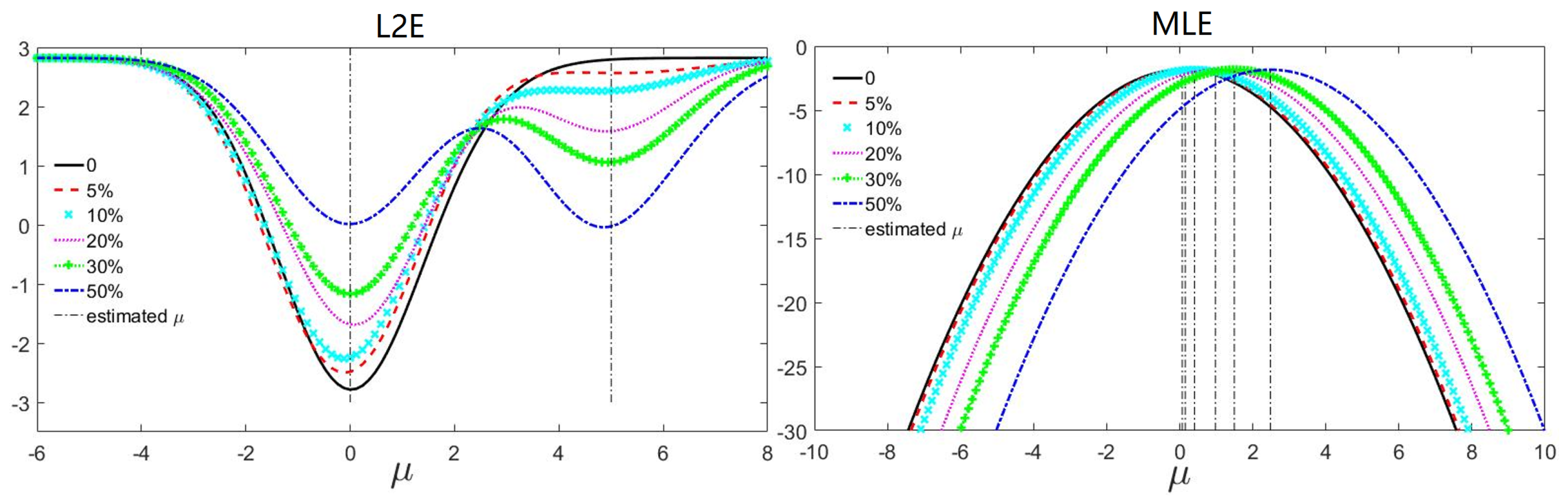
Figure 3.
The robustness comparison between and . We estimate the mean of a normally distributed sample with contaminations of extra samples . The outlier to the inlier ratios are , , , and . The vertical dash lines indicate the extrema. has a global minimum at approximately 0 and a local minimum at approximately 5, both of which conform to the inlier and outlier distributions, respectively. However, the deviation of MLE increases as the ratio grows.
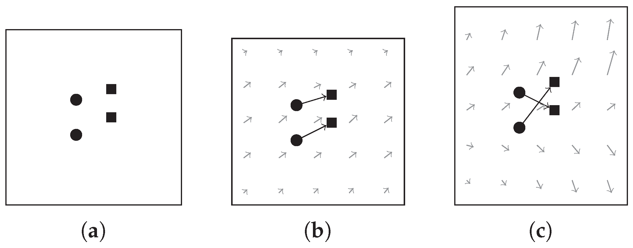
Figure 4.
Illustration of the velocity field. (a): two given point pairs. (b): a coherent velocity field. (c): a velocity field that is less coherent.
Figure 4.
Illustration of the velocity field. (a): two given point pairs. (b): a coherent velocity field. (c): a velocity field that is less coherent.
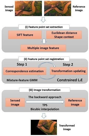
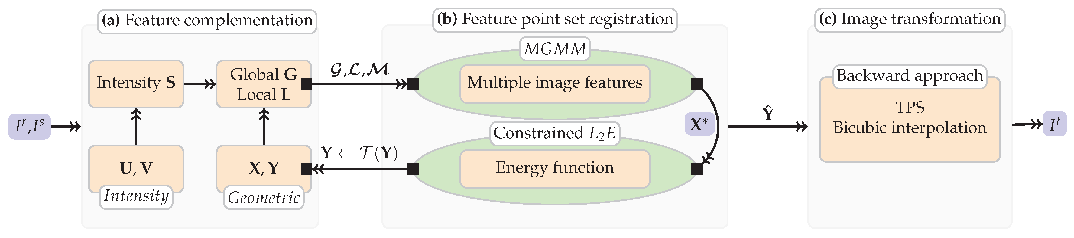
Figure 5.
The summary of our method. (a): Extracting putative corresponding set and SIFT descriptor set using SIFT algorithm, and obtaining two types of discrepancies, i.e., the global and local geometric structure discrepancies and , and intensity information discrepancy . (b): substituting the combined features into the optimization framework and obtaining the transformed point set , note that a loop is included. (c): Image registration based on the backward approach.
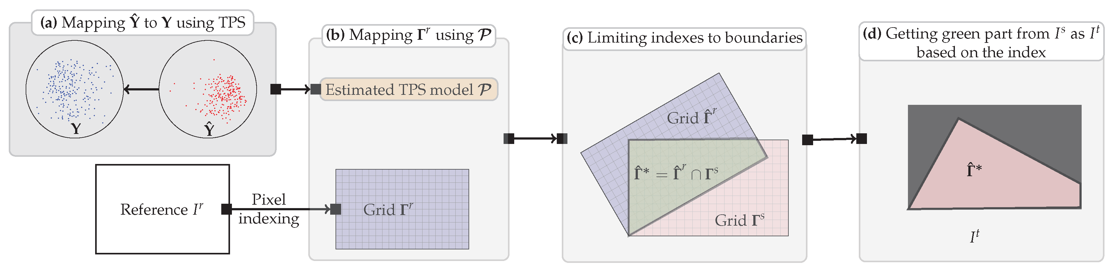
Figure 6.
Illustration of the image transformation and resampling. (a) Computing a TPS transformation model which maps back onto , meanwhile, constructing a grid which is of the same size as ; (b) Mapping using , obtaining ; (c) Limiting indexes to boundaries of ; (d) Getting intensities from within boundaries to generate , each pixel in is determined by the bicubic interpolation.
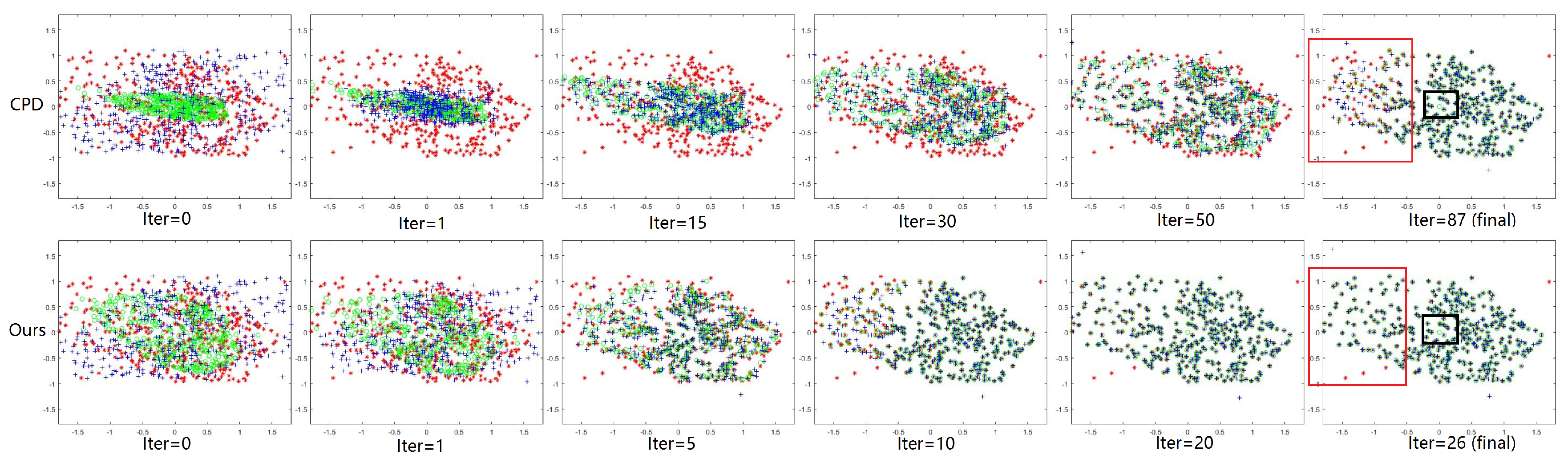
Figure 7.
Demonstration of the advantage of the MGMM. Red *: the target feature point set . Green ∘: the estimated corresponding point set . Blue +: the source feature point set . Upper row and lower row: registration process of CPD and our method. and are extracted from a remote sensing image pair.
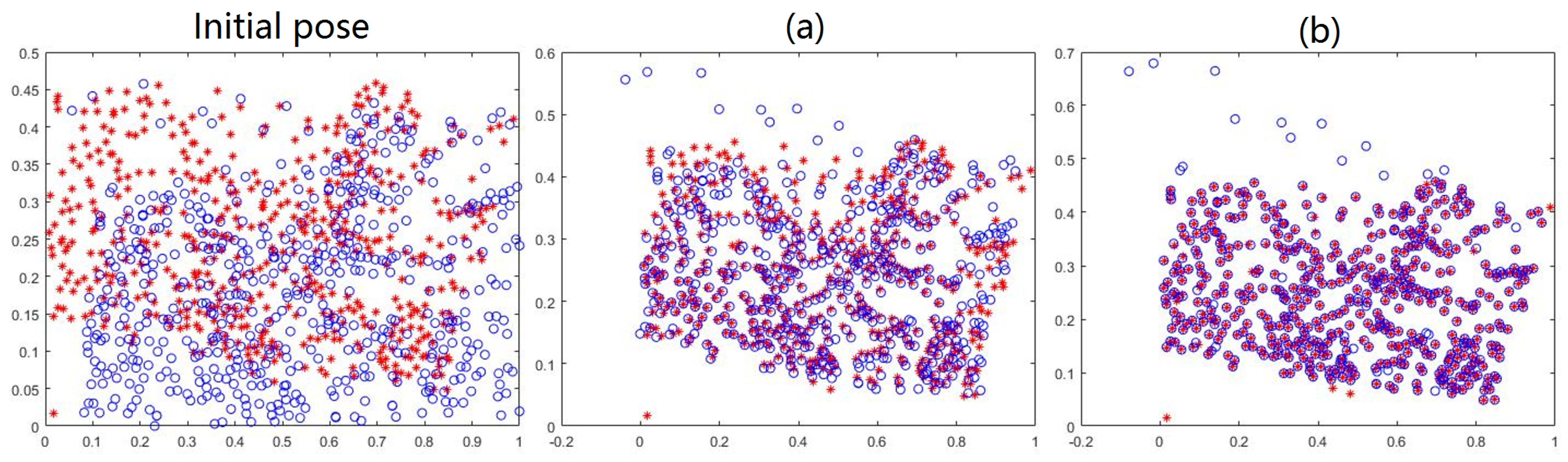
Figure 8.
Examination of the availability of the MGMM. Red *: the target feature point set . Blue ∘: the source feature point set . (a,b) registration result of GMMREG and our method. Obvious deviation exists in the result of GMMREG.
Figure 8.
Examination of the availability of the MGMM. Red *: the target feature point set . Blue ∘: the source feature point set . (a,b) registration result of GMMREG and our method. Obvious deviation exists in the result of GMMREG.
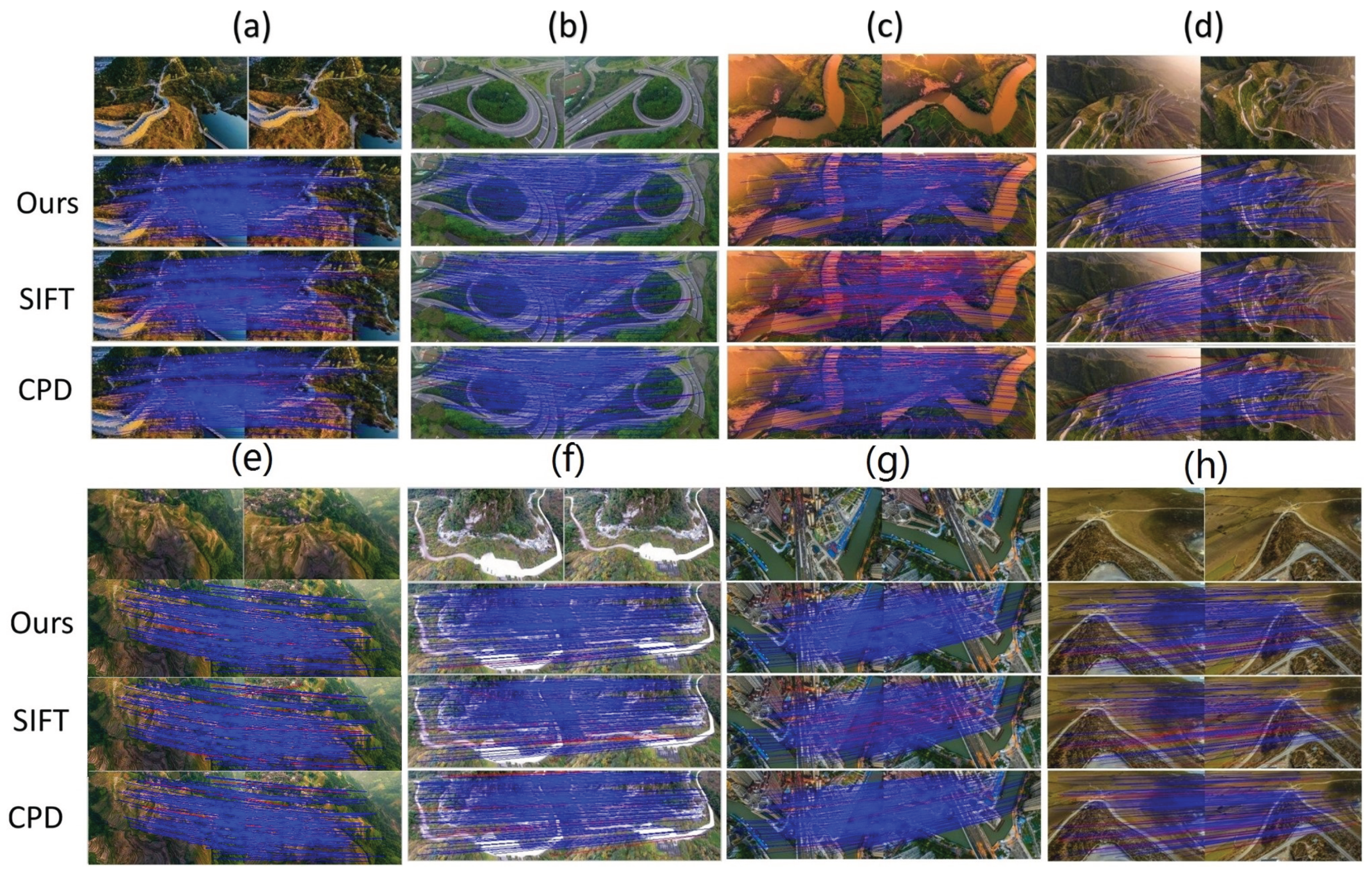
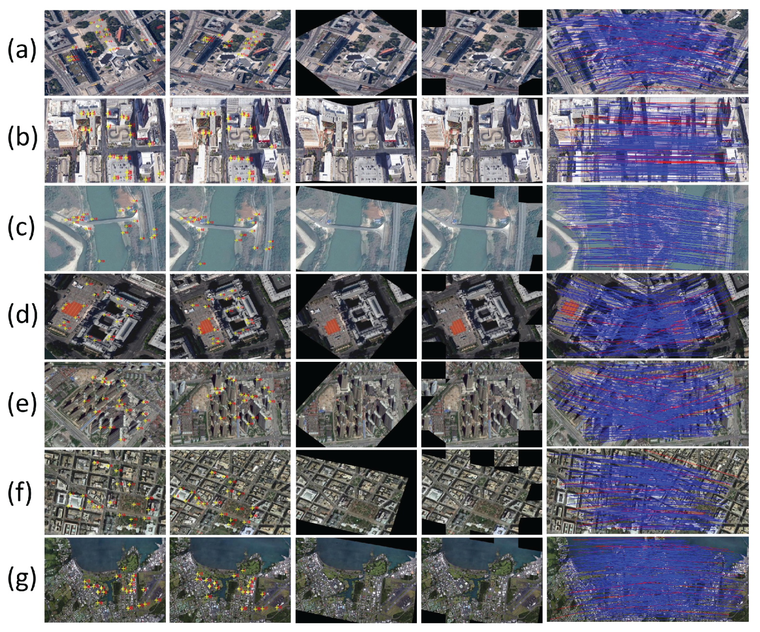
Figure 9.
Feature matching demonstrations on eight typical image pairs of dataset (i) and (ii). For each image pair, rows from the first to the fourth are: the image pair, the results on feature matching of ours, SIFT and CPD, respectively. Blue lines indicate true positive and true negative, red lines indicate false positive and false negative. The PRs of three methods on each image pairs are listed from (a) to (h) as follows. Ours: 99.00, 99.29, 97.31, 97.40, 99.32, 99.62, 98.31, 98.89; SIFT: 85.68, 85.18, 45.12, 60.26, 82.43, 80.34, 82.43, 83.55; CPD: 86.86, 88.14, 85.02, 88.24, 87.22, 85.55, 89.76, 85.23.
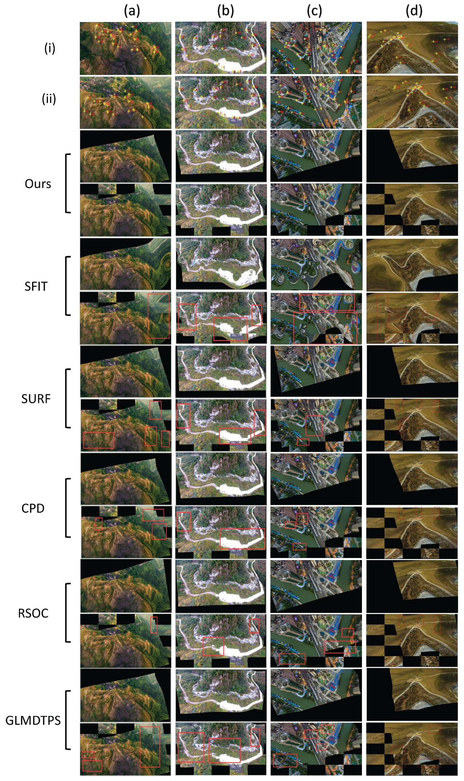
Figure 10.
Registration examples on four typical image pairs from dataset (i). The first two rows: the sensed and reference image, with the yellow crosses denoting the landmarks. Rows from the third to the end are the registration results of ours, SIFT, SURF, CPD, RSOC and GLMDTPS. For each method, the registration results are shown using two rows, with the upper row showing the transformed image, and the lower row showing the checkboard. The registration errors are highlighted using the red rectangles.
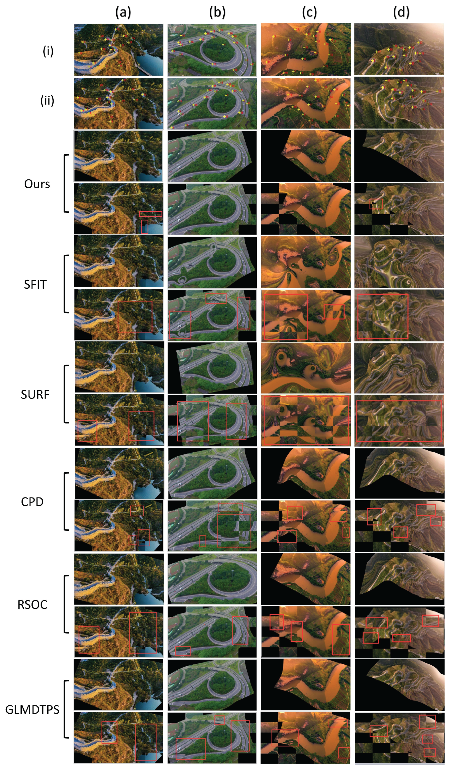
Figure 11.
Registration examples on four typical image pairs from dataset (ii). The first two rows: the sensed and reference image, with the yellow crosses denoting the landmarks. Rows from the third to the end are the registration results of ours, SIFT, SURF, CPD, RSOC and GLMDTPS. For each method, the registration results are shown using two rows, with the upper row showing the transformed image, and the lower row showing the checkboard. The registration errors are highlighted using the red rectangles.
Figure 12.
Registration examples on the seven typical satellite image pairs. From (a) to (g) are: Berlin, Las Vegas, Mekong River, Paris, WuHan, Washington and Hawaii. Columns from the left to the right are: the sensed, reference and transformed images, the checkboards, and the feature matching results. Blue lines indicate true positive and true negative, red lines indicate false positive and false negative.
Table 1.
The experimental design.
Table 1.
The experimental design.
| Series | Criteria | Compared Methods | Datasets Used |
|---|
| I | PR | SIFT, CPD, Ours | (i), (ii) |
| II | All | All | (i), (ii) |
| III | All | Ours | (iii) |
Table 2.
Numbers of the extracted feature points.
Table 2.
Numbers of the extracted feature points.
| Type 1 | Type 2 | Type 3 |
|---|
| 87 to 505 | 30 | 35 to 165 |
Table 3.
Experimental results of series (I). Quantitative comparisons on the mean PR of Type I method are carried out. Bold fonts indicate the best results. All Units are in percentage.
Table 3.
Experimental results of series (I). Quantitative comparisons on the mean PR of Type I method are carried out. Bold fonts indicate the best results. All Units are in percentage.
| Dataset | SIFT | CPD | Ours |
|---|
| (i) | 78.30 | 90.81 | 98.25 |
| (ii) | 72.78 | 90.17 | 97.15 |
Table 4.
Experimental results on series (II). Quantitative comparisons on image registration measured using the mean RMSE, MAE and SD are carried out. Bold fonts indicate the best results. All units are in pixel.
Table 4.
Experimental results on series (II). Quantitative comparisons on image registration measured using the mean RMSE, MAE and SD are carried out. Bold fonts indicate the best results. All units are in pixel.
| | Dataset | SIFT | SURF | CPD | GLMDTPS | RSOC | OURS |
|---|
| RMSE | (i) | 13.5287 | 7.9837 | 3.2386 | 3.0152 | 2.2737 | 1.0171 |
| | (ii) | 11.4466 | 7.0627 | 7.2645 | 5.5991 | 4.1743 | 1.4331 |
| MAE | (i) | 16.0080 | 12.2803 | 7.5404 | 7.1459 | 6.4448 | 4.0271 |
| | (ii) | 14.2989 | 9.8411 | 10.3778 | 9.1102 | 7.3585 | 3.9188 |
| SD | (i) | 14.1826 | 10.2241 | 5.8594 | 5.4353 | 4.8013 | 3.1957 |
| | (ii) | 11.9613 | 8.2523 | 4.3619 | 7.6531 | 5.7844 | 3.0021 |
Table 5.
Experimental results on series (III). Quantitative tests on feature matching and image registration are carried out to examine the availability and robustness of our method using the PR, RMSE, MAE and SD. (a) to (g): results on the corresponding pairs of
Figure 12. Mean: the mean of results on all image pairs of dataset (iii). For the PR, the units are in percentage, for the RMSE, MAE and SD, the units are in pixel.
| | (a) | (b) | (c) | (d) | (e) | (f) | (g) | Mean |
|---|
| 96.88 | 96.77 | 95.97 | 95.77 | 95.09 | 98.19 | 95.57 | 96.54 |
| 0.8358 | 1.3963 | 1.9556 | 1.4272 | 0.7743 | 1.4342 | 0.3171 | 1.1628 |
| 2.1458 | 4.0208 | 2.9097 | 1.9317 | 2.5778 | 2.3542 | 2.2958 | 2.6051 |
| 1.8562 | 2.5498 | 2.5171 | 1.8061 | 2.1429 | 2.0098 | 2.0717 | 2.1362 |


