
Assessment of Satellite-Derived Surface Reflectances by NASA’s CAR Airborne Radiometer over Railroad Valley Playa


 , ,
, ,
Abstract
:
1. Introduction
2. Method
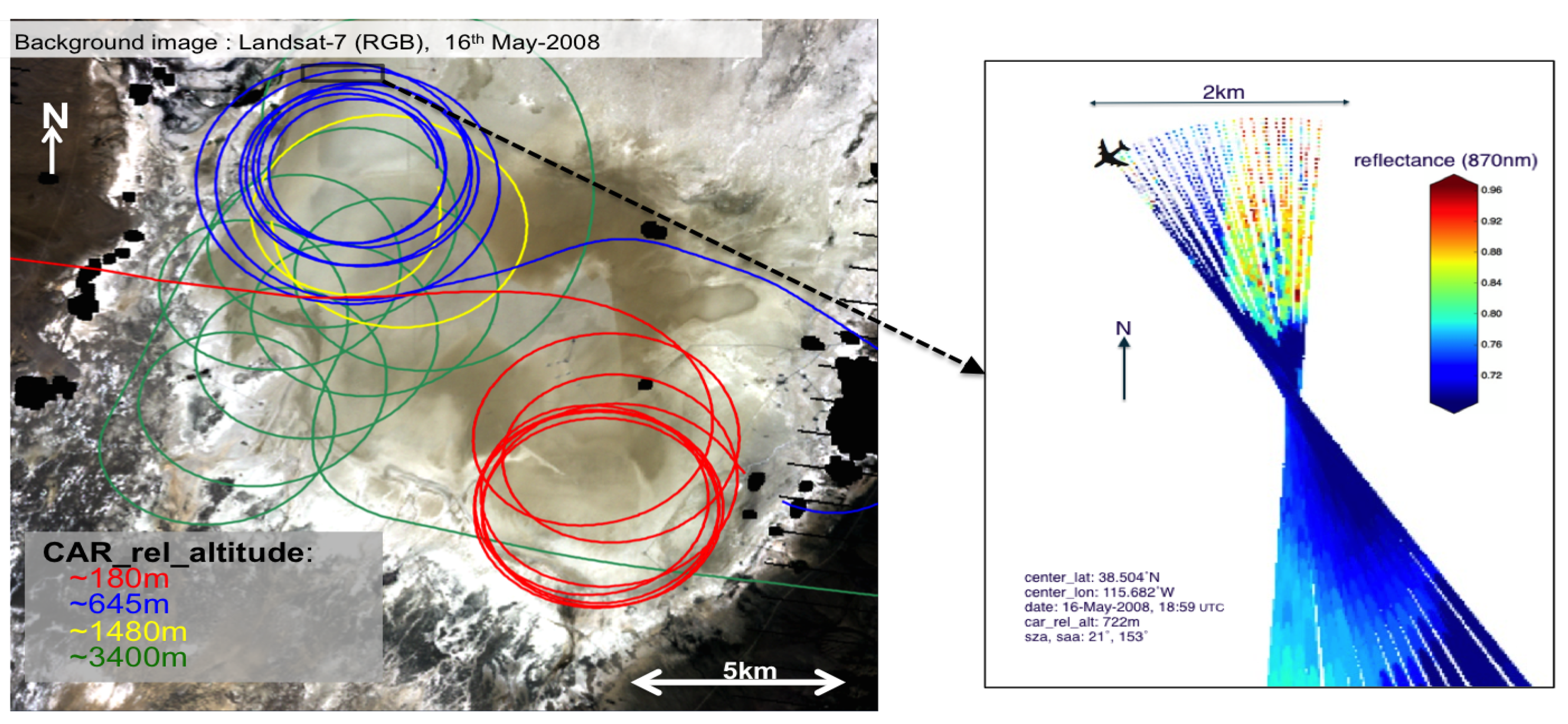
2.1. Site
2.2. Data
2.2.1. CAR Data
2.2.2. Satellite Data
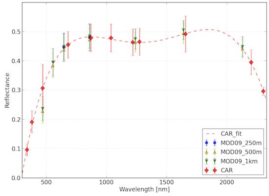
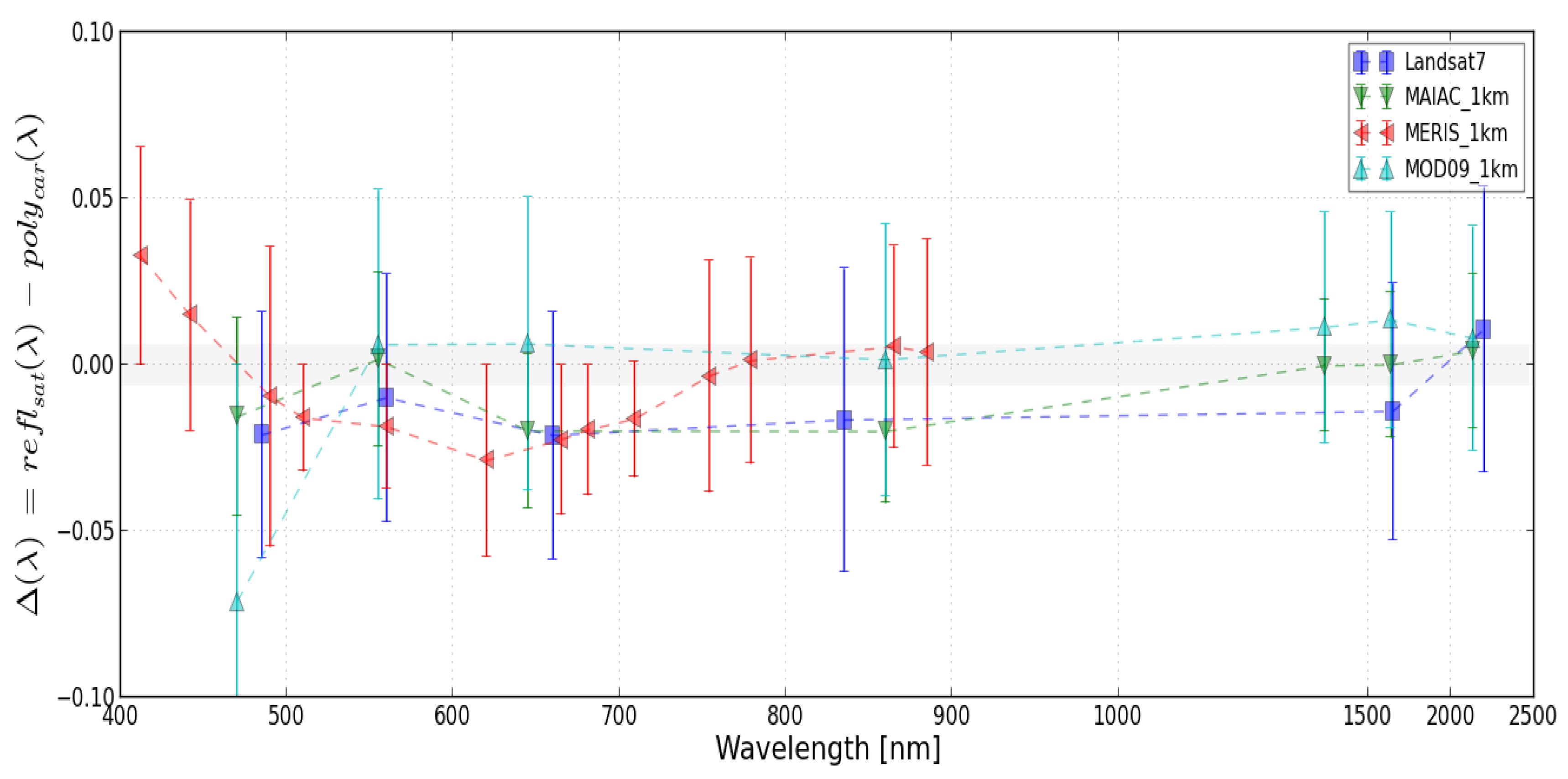
- MOD09: Surface reflectance derived from the top of atmosphere (ToA) data of Terra/MODIS, collection 6, at three spatial resolutions: 250 m (for two spectral bands only), 500 m and 1 km [22]. The atmospheric correction of MOD09 is performed through Second Simulation of a Satellite Signal in the Solar Spectrum (6S) radiative transfer models [23,24] that take as input ToA radiance data, water vapor, ozone, geopotential height, aerosol optical thickness, and digital elevation.
- MAIAC: MultiAngle Implementation of Atmospheric Correction [25] is another product of surface reflectance derived from Terra/MODIS ToA radiance data at two spatial resolutions: 500 m and 1 km. MAIAC computes Ross–Thick Li-Sparse (RTLS) BRDF parameters and then extracts BRF (Bidirectional Reflectance Factor) when the land surface is stable or changes slowly; otherwise, MAIAC follows the MODIS operational BRDF algorithm. MAIAC deploys a moving window of up to 16 days over MODIS ToA radiance data.
- MERIS: Medium Resolution Imaging Spectrometer, onboard the ENVISAT platform [26]. The atmospheric correction of MERIS is modeled using a simple single scattering model assuming that the atmospheric path radiance and absorption can be separated into two components, Rayleigh and aerosol in such a way that aerosol component is modeled by a simple angstrom exponent [27].
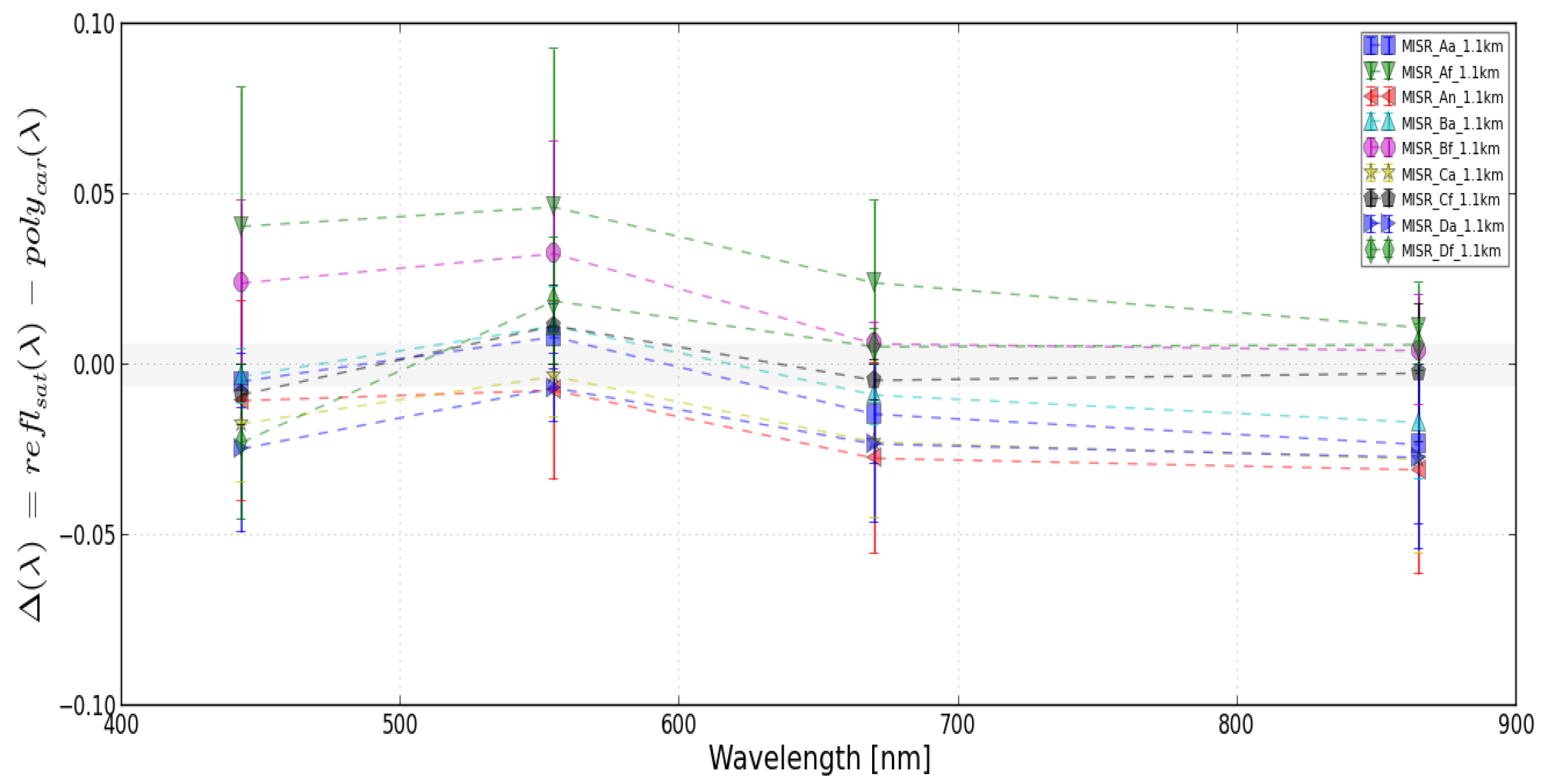
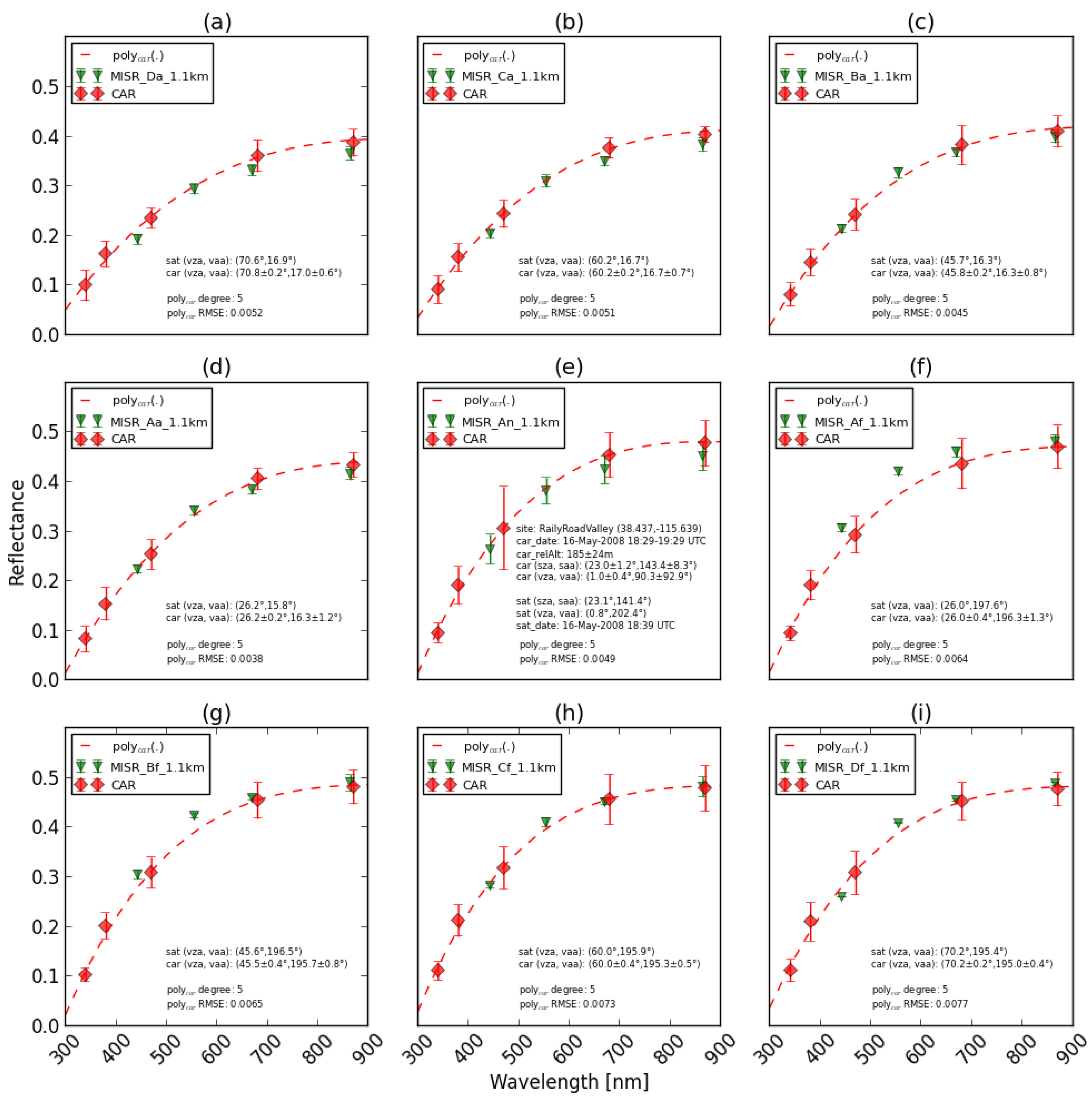
- MISR: Multi-angle Imaging SpectroRadiometer is a multi-angular spaceborne instrument onboard the Terra platform. It deploys nine cameras at different view angles, over four spectral bands: nm, nm, nm, and nm. The MISR product that was used here is MISR_AM1_AS_LAND [31]. In this product ToA radiance data are first atmospherically corrected for generating the Hemispherical Directional Reflectance Factor (HDRF) and Bi-Hemispherical Reflectance (BHR) and then further atmospheric correction is applied on the two variables to remove all diffuse components and then generate BRF [13]. The accuracy of MISR’s atmospheric correction is strongly related to the accuracy of MISR’s aerosol product, which is considered accurate thanks to the nine view cameras, despite the fact that the aerosol product has a much lower spatial resolution (17.6 km × 17.6 km) [32].
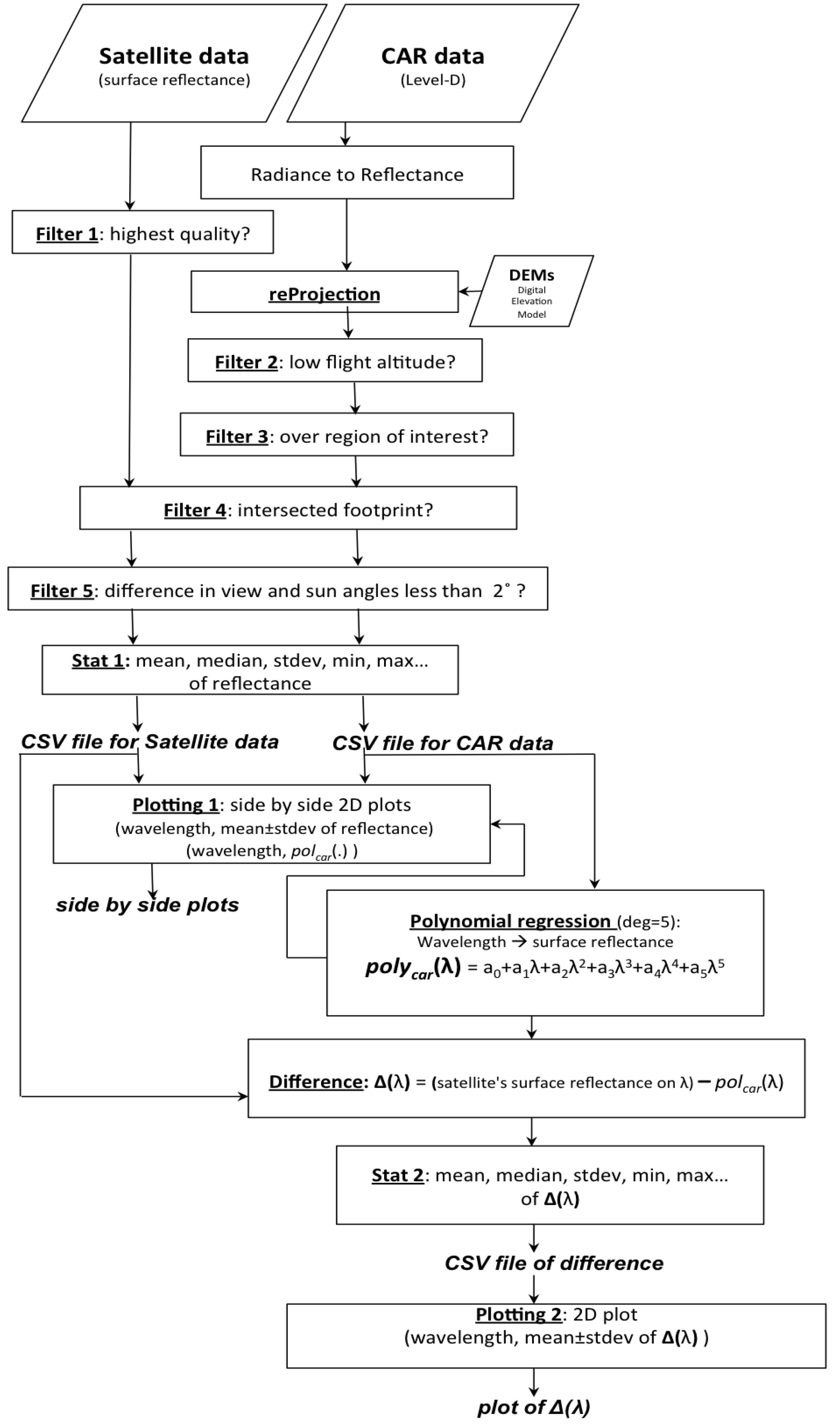
2.3. Assessment Method
3. Results
4. Discussion
5. Conclusions
Acknowledgments
Author Contributions
Conflicts of Interest
Abbreviations
| BRF | B-directional Reflectance Factor |
| CAR | Cloud Absorption Radiometer |
| IFOV | Instantaneous Field Of View |
| MAIAC | Multi-Angle Implementation of Atmospheric Correction |
| MERIS | MEdium Resolution Imaging Spectrometer |
| MISR | Multi-angle Imaging SpectroRadiometer |
| MODIS | MODerate resolution Imaging Spectroradiometer |
| SAA | Solar Azimuth Angle |
| SZA | Solar Zenith Angle |
| ToA | Top of Atmosphere |
| VAA | View Azimuth Angle |
| VZA | View Zenith Angle |
References
- Ward, S. The Earth Observation Handbook. Committee on Earth Observation Satellites. Available online: www.eohandbook.com (accessed on November 2015).
- Yang, J.; Gong, P.; Fu, R.; Zhang, M.; Chen, J.; Liang, S.; Xu, B.; Shi, J.; Dickinson, R. The role of satellite remote sensing in climate change studies. Nat. Clim. Chang. 2013, 3, 875–883. [Google Scholar] [CrossRef]
- Marchetti, P.G.; Soille, P.; Bruzzone, L. A Special Issue on Big Data from Space for Geoscience and Remote Sensing [From the Guest Editors]. IEEE Geosci. Remote Sens. Mag. 2016, 4, 7–9. [Google Scholar] [CrossRef]
- Lin, J.; Liu, M.; Xin, J.; Boersma, K.; Spurr, R.; Martin, R.; Zhang, Q. Influence of aerosols and surface reflectance on satellite NO2 retrieval: seasonal and spatial characteristics and implications for NOx emission constraints. Atmos. Chem. Phys. 2015, 15, 11217–11241. [Google Scholar] [CrossRef]
- Foody, G.M.; Atkinson, P.M. Uncertainty in Remote Sensing And GIS; Wiley Online Library: New York, NY, USA, 2002. [Google Scholar]
- Mannschatz, T.; Pflug, B.; Borg, E.; Feger, K.H.; Dietrich, P. Uncertainties of LAI estimation from satellite imaging due to atmospheric correction. Remote Sens. Environ. 2014, 153, 24–39. [Google Scholar] [CrossRef]
- Schaepman-Strub, G.; Schaepman, M.; Painter, T.; Dangel, S.; Martonchik, J. Reflectance quantities in optical remote sensing—Definitions and case studies. Remote Sens. Environ. 2006, 103, 27–42. [Google Scholar] [CrossRef]
- Bruegge, C.J.; Helmlinger, M.C.; Conel, J.E.; Gaitley, B.J.; Abdou, W.A. PARABOLA III: A sphere-scanning radiometer for field determination of surface anisotropic reflectance functions. Remote Sens. Rev. 2000, 19, 75–94. [Google Scholar] [CrossRef]
- Sandmeier, S.R.; Itten, K.I. A field goniometer system (FIGOS) for acquisition of hyperspectral BRDF data. IEEE Trans. Geosci. Remote Sens. 1999, 37, 978–986. [Google Scholar] [CrossRef]
- Pegrum-Browning, H.; Fox, N.; Milton, E. The NPL Gonio RAdiometric Spectrometer System (GRASS). In Proceedings of the Remote Sensing and Photogrammetry Society Conference: “Measuring Change in the Earth System”, University of Exeter, Exeter, UK, 15–17 September 2008. [Google Scholar]
- Liang, S.; Fang, H.; Chen, M.; Shuey, C.J.; Walthall, C.; Daughtry, C.; Morisette, J.; Schaaf, C.; Strahler, A. Validating MODIS land surface reflectance and albedo products: Methods and preliminary results. Remote Sens. Environ. 2002, 83, 149–162. [Google Scholar] [CrossRef]
- Hook, S.J.; Myers, J.J.; Thome, K.J.; Fitzgerald, M.; Kahle, A.B. The MODIS/ASTER airborne simulator (MASTER)—A new instrument for earth science studies. Remote Sens. Environ. 2001, 76, 93–102. [Google Scholar] [CrossRef]
- Diner, D.J.; Barge, L.M.; Bruegge, C.J.; Chrien, T.G.; Conel, J.E.; Eastwood, M.L.; Garcia, J.D.; Hernandez, M.A.; Kurzweil, C.G.; Ledeboer, W.C.; et al. The Airborne Multi-angle Imaging SpectroRadiometer (AirMISR): Instrument description and first results. IEEE Trans. Geosci. Remote Sens. 1998, 36, 1339–1349. [Google Scholar] [CrossRef]
- Leroy, M.; Bréon, F.M. Angular signatures of surface reflectances from airborne POLDER data. Remote Sens. Environ. 1996, 57, 97–107. [Google Scholar] [CrossRef]
- Irons, J.R.; Ranson, K.; Williams, D.L.; Irish, R.R.; Huegel, F.G. An off-nadir-pointing imaging spectroradiometer for terrestrial ecosystem studies. IEEE Trans. Geosci. Remote Sens. 1991, 29, 66–74. [Google Scholar] [CrossRef]
- Abdou, W.A.; Conel, J.E.; Pilorz, S.H.; Helmlinger, M.C.; Bruegge, C.J.; Gaitley, B.J.; Ledeboer, W.C.; Martonchik, J.V. Vicarious calibration: A reflectance-based experiment with AirMISR. Remote Sens. Environ. 2001, 77, 338–353. [Google Scholar] [CrossRef]
- Gatebe, C.K.; King, M.D. Airborne spectral BRDF of various surface types (ocean, vegetation, snow, desert, wetlands, cloud decks, smoke layers) for remote sensing applications. Remote Sens. Environ. 2016, 179, 131–148. [Google Scholar] [CrossRef]
- Román, M.O.; Gatebe, C.K.; Schaaf, C.B.; Poudyal, R.; Wang, Z.; King, M.D. Variability in surface BRDF at different spatial scales (30 m–500 m) over a mixed agricultural landscape as retrieved from airborne and satellite spectral measurements. Remote Sens. Environ. 2011, 115, 2184–2203. [Google Scholar] [CrossRef]
- Román, M.O.; Gatebe, C.K.; Shuai, Y.; Wang, Z.; Gao, F.; Masek, J.G.; He, T.; Liang, S.; Schaaf, C.B. Use of in situ and airborne multiangle data to assess MODIS-and Landsat-based estimates of directional reflectance and albedo. IEEE Trans. Geosci. Remote Sens. 2013, 51, 1393–1404. [Google Scholar] [CrossRef]
- Scott, K.P.; Thome, K.J.; Brownlee, M.R. Evaluation of the Railroad Valley Playa for use in vicarious calibration. Proc. SPIE 1996, 2818, 158–166. [Google Scholar]
- Van De Hulst, H.C. Multiple Light Scattering: Tables, Formulas and Applications; Academic Press: New York, NY, USA, 1980. [Google Scholar]
- MODIS Surface Reflectance User’s Guide, Collection 6. Available online: http://modis-sr.ltdri.org/guide/MOD09_UserGuidev1.4.pdf (accessed on 1 May 2015).
- Vermote, E.F.; Tanré, D.; Deuze, J.L.; Herman, M.; Morcette, J.J. Second simulation of the satellite signal in the solar spectrum, 6S: An overview. IEEE Trans. Geosci. Remote Sens. 1997, 35, 675–686. [Google Scholar] [CrossRef]
- Vermote, E.F.; Kotchenova, S. Atmospheric correction for the monitoring of land surfaces. J. Geophys. Res. Atmos. 2008, 113. [Google Scholar] [CrossRef]
- Lyapustin, A.I.; Wang, Y.; Laszlo, I.; Hilker, T.; Hall, F.G.; Sellers, P.J.; Tucker, C.J.; Korkin, S.V. Multi-angle implementation of atmospheric correction for MODIS (MAIAC): 3. Atmospheric correction. Remote Sens. Environ. 2012, 127, 385–393. [Google Scholar] [CrossRef]
- MERIS Product Handbook. Available online: http://envisat.esa.int/handbooks/meris/CNTR.html (accessed on 1 August 2011).
- Moore, G.; Lavender, S. Algorithm Identification: Case II. S Bright Pixel Atmospheric Correction (MERIS ATBD 2.6). 2011. Available online: https://earth.esa.int/documents/700255/2042855/MERISATBD2.6v5.0+-+2011.pdf (accessed on 1 August 2011).
- Masek, J.G.; Vermote, E.F.; Saleous, N.E.; Wolfe, R.; Hall, F.G.; Huemmrich, K.F.; Gao, F.; Kutler, J.; Lim, T.K. A Landsat surface reflectance dataset for North America, 1990–2000. IEEE Geosci. Remote Sens. Lett. 2006, 3, 68–72. [Google Scholar] [CrossRef]
- Landsat 4-7 Surface Reflectance (LEDAPS) Product, How Published. Available online: https://landsat.usgs.gov/sites/default/files/documents/ledaps_product_guide.pdf (accessed on 30 September 2016).
- Ouaidrari, H.; Vermote, E.F. Operational atmospheric correction of Landsat TM data. Remote Sens. Environ. 1999, 70, 4–15. [Google Scholar] [CrossRef]
- MISR Science Data Product Guide. Available online: https://eosweb.larc.nasa.gov/sites/default/files/project/misr/guide/MISR_Science_DataProduct_Guide.pdf (accessed on 7 May 2012).
- Diner, D.J.; Martonchik, J.V.; Kahn, R.A.; Pinty, B.; Gobron, N.; Nelson, D.L.; Holben, B.N. Using angular and spectral shape similarity constraints to improve MISR aerosol and surface retrievals over land. Remote Sens. Environ. 2005, 94, 155–171. [Google Scholar] [CrossRef]
- Wanner, W.; Li, X.; Strahler, A. On the derivation of kernels for kernel-driven models of bidirectional reflectance. J. Geophys. Res. Atmos. 1995, 100, 21077–21089. [Google Scholar] [CrossRef]


| CAR’s Spectral Bands [nm] | ||||||
|---|---|---|---|---|---|---|
| * | * | * | * | * | * | * |
| * | * | |||||
| Product | Num of Samples | Spatial Resolution | SZA | SAA | VZA | VAA | Reflectance: (band [nm], mean, stdev) |
|---|---|---|---|---|---|---|---|
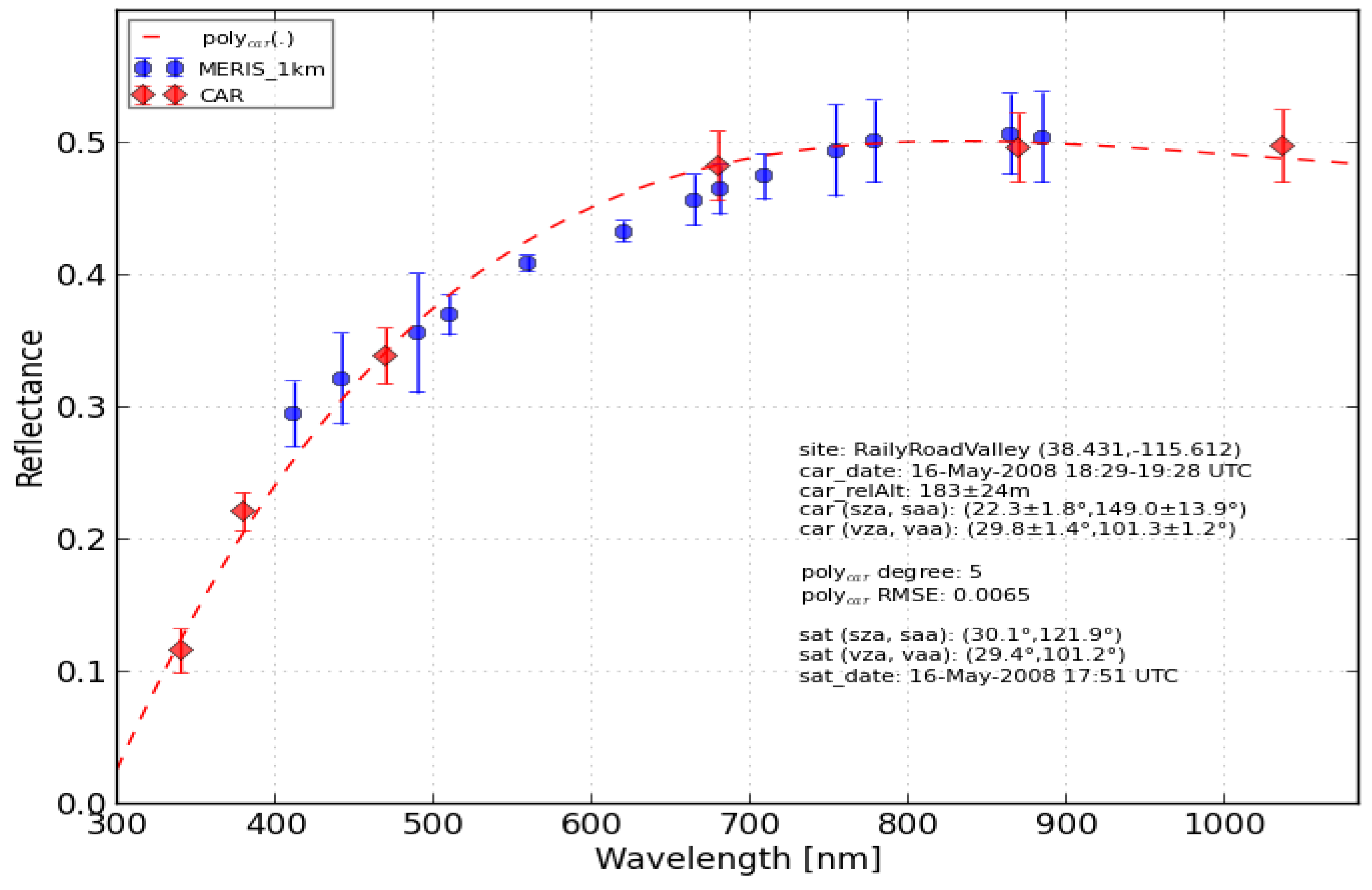
| MERIS_1 km | 2 | 1 km × 1 km | 30.1° | 121.9° | 29.4° | 101.2° | (412, 0.295, 0.025), (442, 0.322, 0.035), (490, 0.356, 0.045), (510, 0.37, 0.015), (560, 0.408, 0.006), (620, 0.433, 0.008), (665, 0.457, 0.019), (681, 0.464, 0.019), (709, 0.474, 0.017), (754, 0.494, 0.035), (779, 0.501, 0.031), (865, 0.507, 0.03), (885, 0.504, 0.034) |
| CAR | 230 | 4 m × 4 m | 22.3 ± 1.8° | 149.0 ± 13.9° | 29.8 ± 1.4° | 101.3 ± 1.2° | (340, 0.116, 0.017), (380, 0.221, 0.015), (470, 0.339, 0.021), (680, 0.482, 0.026), (870, 0.496, 0.026), (1037, 0.498, 0.027), (1219, 0.473, 0.028), (1275, 0.47, 0.028), (1657, 0.469, 0.018), (2202, 0.424, 0.016) |
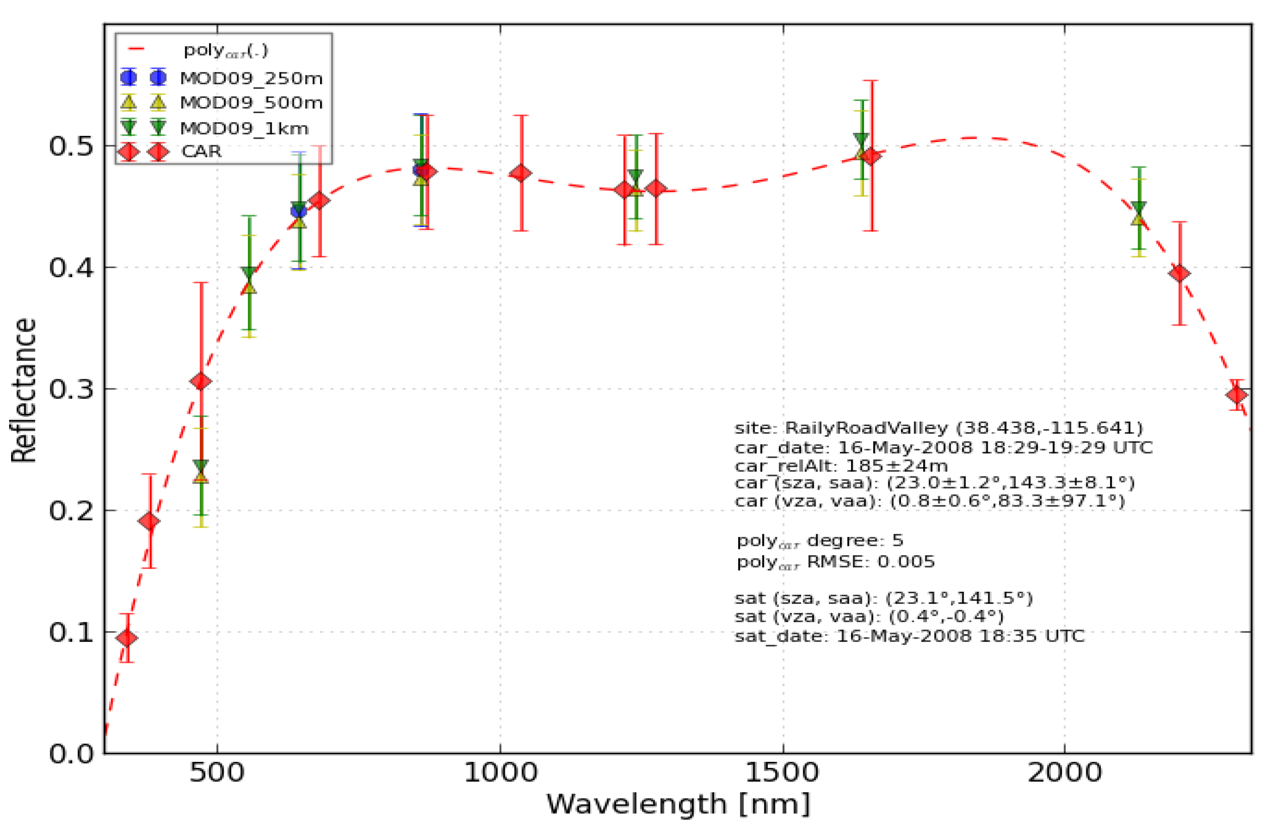
| MOD09_1 km | 46 | 1 km × 1 km | 23.1° | 141.5° | 0.4° | 24.5° | (470, 0.237, 0.041), (555, 0.395, 0.047), (645, 0.449, 0.044), (860, 0.484, 0.041), (1240, 0.475, 0.035), (1640, 0.505, 0.032), (2130, 0.449, 0.034) |
| MOD09_500 m | 112 | 500 m × 500 m | 23.1° | 141.5° | 0.3° | 28.0° | (470, 0.227, 0.041), (555, 0.384, 0.042), (645, 0.437, 0.04), (860, 0.472, 0.037), (1240, 0.463, 0.034), (1640, 0.494, 0.034), (2130, 0.441, 0.032) |
| MOD09_250 m | 256 | 250 m × 250 m | 23.1° | 141.5° | 0.4° | −0.4° | (645, 0.447, 0.048), (860, 0.48, 0.046) |
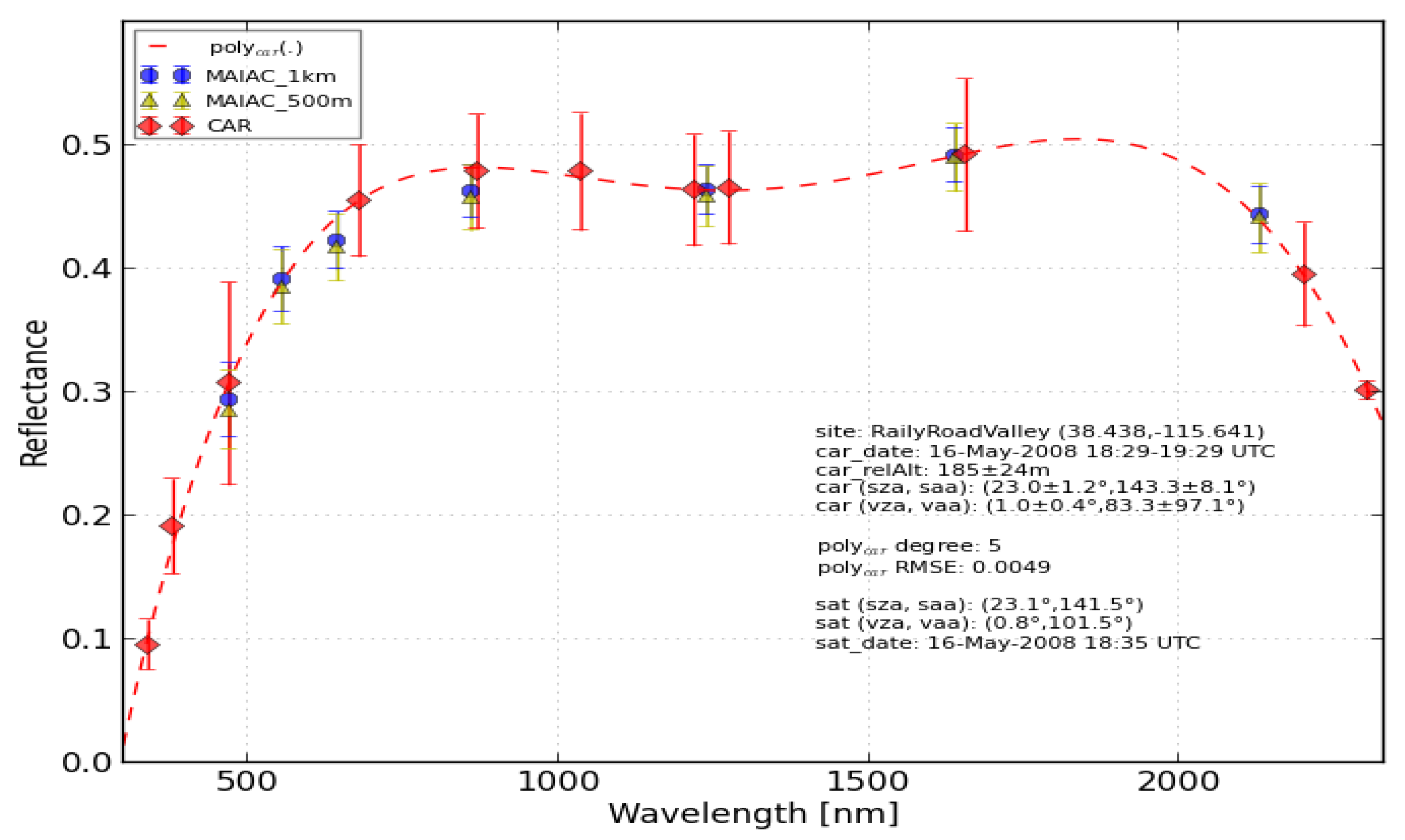
| CAR | 5863 | 3 m × 3 m | 23.0 ± 1.2° | 143.3 ± 8.1° | 0.8 ± 0.6° | 83.3 ± 97.1° | (340, 0.096, 0.02), (380, 0.191, 0.038), (470, 0.307, 0.081), (680, 0.455, 0.045), (870, 0.478, 0.046), (1037, 0.478, 0.048), (1219, 0.463, 0.045), (1275, 0.465, 0.046), (1657, 0.492, 0.062), (2202, 0.395, 0.042), (2303, 0.295, 0.013) |
| MAIAC_1 km | 28 | 1 km × 1 km | 23.1° | 141.5° | 0.8° | 101.5° | (470, 0.293, 0.03), (555, 0.392, 0.026), (645, 0.423, 0.023), (860, 0.462, 0.022), (1240, 0.464, 0.02), (1640, 0.492, 0.022), (2130, 0.443, 0.023) |
| MAIAC_500 m | 88 | 500 m × 500 m | 23.1° | 141.5° | 0.8° | 105.6° | (470, 0.286, 0.032), (555, 0.385, 0.03), (645, 0.417, 0.027), (860, 0.457, 0.026), (1240, 0.458, 0.024), (1640, 0.49, 0.028), (2130, 0.441, 0.028) |
| CAR | 4410 | 3m × 3m | 23.0 ± 1.2° | 143.3 ± 8.1° | 1.0 ± 0.4° | 83.3 ± 97.1° | (340, 0.096, 0.02), (380, 0.191, 0.038), (470, 0.307, 0.082), (680, 0.455, 0.045), (870, 0.478, 0.046), (1037, 0.478, 0.047), (1219, 0.463, 0.045), (1275, 0.465, 0.046), (1657, 0.492, 0.062), (2202, 0.395, 0.042), (2303, 0.302, 0.008) |
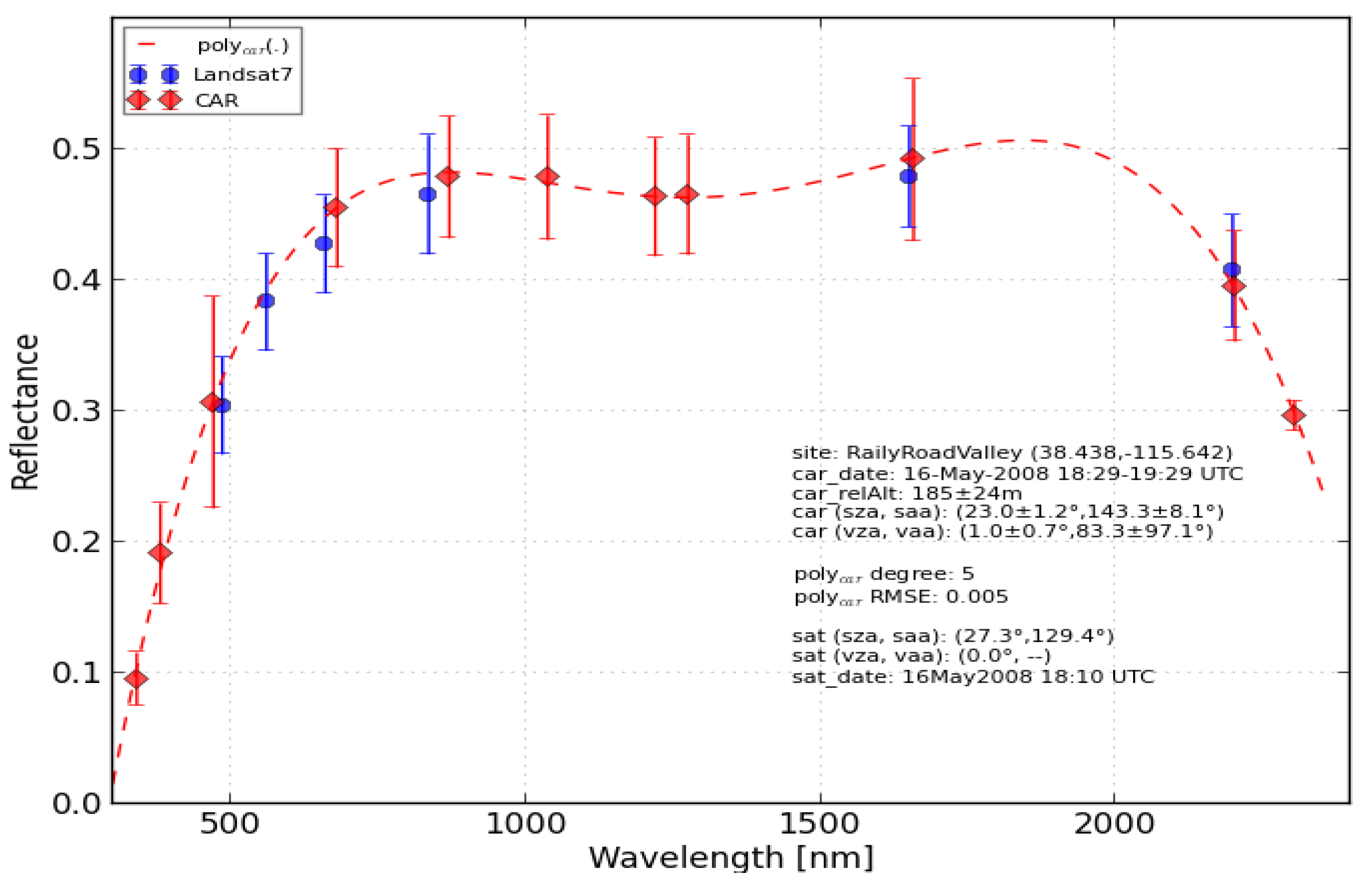
| Landsat7 | 1472 | 30 m × 30 m | 27.3° | 129.4° | 0.0° | - | (485, 0.304, 0.037), (560, 0.383, 0.037), (660, 0.427, 0.037), (835, 0.465, 0.046), (1650, 0.479, 0.039), (2198, 0.407, 0.043) |
| CAR | 7355 | 3 m × 3 m | 23.0 ± 1.2° | 143.3 ± 8.1° | 1.0 ± 0.7° | 83.3 ± 97.1° | (340, 0.096, 0.02), (380, 0.191, 0.038), (470, 0.307, 0.081), (680, 0.455, 0.045), (870, 0.478, 0.046), (1037, 0.478, 0.047), (1219, 0.463, 0.045), (1275, 0.465, 0.046), (1657, 0.492, 0.062), (2202, 0.395, 0.042), (2303, 0.297, 0.011) |
| MISR.Aa_1.1 km | 5 | 1.1 km × 1.1 km | 23.2° | 141.5° | 26.2° | 15.8° | (443, 0.224, 0.008), (555, 0.342, 0.01), (670, 0.384, 0.008), (865, 0.416, 0.012) |
| CAR | 58 | 4 m × 4 m | 22.8 ± 1.4° | 144.5 ± 8.9° | 26.2 ± 0.2° | 16.3 ± 1.2° | (340, 0.083, 0.025), (380, 0.154, 0.033), (470, 0.254, 0.03), (680, 0.406, 0.021), (870, 0.434, 0.024), (1037, 0.441, 0.024), (1219, 0.431, 0.021), (1275, 0.426, 0.019), (1657, 0.485, 0.015), (2202, 0.356, 0.02) |
| MISR.Af_1.1 km | 3 | 1.1 km × 1.1 km | 23.2° | 141.2° | 26.0° | 197.6° | (443, 0.307, 0.008), (555, 0.421, 0.008), (670, 0.46, 0.011), (865, 0.482, 0.013) |
| CAR | 66 | 4 m × 3 m | 23.3 ± 0.6° | 140.9 ± 2.4° | 26.0 ± 0.4° | 196.3 ± 1.3° | (340, 0.094, 0.015), (380, 0.191, 0.029), (470, 0.293, 0.037), (680, 0.436, 0.051), (870, 0.47, 0.043), (1037, 0.476, 0.043), (1219, 0.458, 0.042), (1275, 0.46, 0.043), (1657, 0.446, 0.042), (2202, 0.413, 0.034) |
| MISR.An_1.1 km | 40 | 1.1 km × 1.1 km | 23.1° | 141.4° | 0.8° | 202.4° | (443, 0.264, 0.029), (555, 0.382, 0.026), (670, 0.424, 0.028), (865, 0.451, 0.028) |
| CAR | 4233 | 3 m × 3 m | 23.0 ± 1.2° | 143.4 ± 8.3° | 1.0 ± 0.4° | 90.3 ± 92.9° | (340, 0.095, 0.02), (380, 0.191, 0.038), (470, 0.306, 0.083), (680, 0.454, 0.045), (870, 0.478, 0.046), (1037, 0.477, 0.047), (1219, 0.463, 0.045), (1275, 0.464, 0.046), (1657, 0.49, 0.062), (2202, 0.395, 0.042), (2303, 0.302, 0.008) |
| MISR.Ba_1.1 km | 5 | 1.1 km × 1.1 km | 23.2° | 141.5° | 45.7° | 16.3° | (443, 0.213, 0.008), (555, 0.326, 0.011), (670, 0.367, 0.008), (865, 0.4, 0.013) |
| CAR | 44 | 7 m × 5 m | 22.8 ± 1.5° | 144.8 ± 9.3° | 45.8 ± 0.2° | 16.3 ± 0.8° | (340, 0.081, 0.023), (380, 0.146, 0.027), (470, 0.242, 0.031), (680, 0.382, 0.04), (870, 0.409, 0.032), (1037, 0.426, 0.029), (1219, 0.416, 0.027), (1275, 0.407, 0.027), (1657, 0.453, 0.047), (2202, 0.352, 0.017) |
| MISR.Bf_1.1 km | 3 | 1.1 km × 1.1 km | 23.2° | 141.2° | 45.6° | 196.5° | (443, 0.305, 0.009), (555, 0.424, 0.005), (670, 0.458, 0.005), (865, 0.49, 0.016) |
| CAR | 42 | 6 m × 4 m | 23.3 ± 0.6° | 140.8 ± 2.4° | 45.5 ± 0.4° | 195.7 ± 0.8° | (340, 0.103, 0.013), (380, 0.201, 0.026), (470, 0.309, 0.03), (680, 0.454, 0.036), (870, 0.482, 0.034), (1037, 0.493, 0.034), (1219, 0.476, 0.035), (1275, 0.476, 0.035), (1657, 0.467, 0.034), (2202, 0.43, 0.027) |
| MISR.Ca_1.1 km | 5 | 1.1 km × 1.1 km | 23.2° | 141.5° | 60.2° | 16.7° | (443, 0.203, 0.008), (555, 0.31, 0.012), (670, 0.349, 0.009), (865, 0.383, 0.014) |
| CAR | 32 | 14 m × 7 m | 22.5 ± 1.6° | 146.5 ± 10.3° | 60.2 ± 0.2° | 16.7 ± 0.7° | (340, 0.091, 0.028), (380, 0.156, 0.028), (470, 0.244, 0.027), (680, 0.377, 0.021), (870, 0.404, 0.016), (1037, 0.42, 0.015), (1219, 0.407, 0.014), (1275, 0.399, 0.016), (1657, 0.452, 0.021), (2202, 0.342, 0.015) |
| MISR.Cf_1.1 km | 3 | 1.1 km × 1.1 km | 23.2° | 141.2° | 60.0° | 195.9° | (443, 0.281, 0.004), (555, 0.41, 0.008), (670, 0.45, 0.006), (865, 0.481, 0.02) |
| CAR | 30 | 12 m × 6 m | 23.2 ± 0.6° | 141.1 ± 2.4° | 60.0 ± 0.4° | 195.3 ± 0.5° | (340, 0.11, 0.018), (380, 0.212, 0.032), (470, 0.318, 0.042), (680, 0.456, 0.051), (870, 0.479, 0.046), (1037, 0.491, 0.045), (1219, 0.47, 0.043), (1275, 0.469, 0.043), (1657, 0.444, 0.016), (2202, 0.44, 0.024) |
| MISR.Da_1.1 km | 5 | 1.1 km × 1.1 km | 23.2° | 141.5° | 70.6° | 16.9° | (443, 0.192, 0.01), (555, 0.294, 0.01), (670, 0.332, 0.011), (865, 0.366, 0.014) |
| CAR | 28 | 32 m × 10 m | 22.8 ± 1.6° | 145.3 ± 10.5° | 70.8 ± 0.2° | 17.0 ± 0.6° | (340, 0.1, 0.031), (380, 0.163, 0.026), (470, 0.235, 0.02), (680, 0.361, 0.032), (870, 0.387, 0.027), (1037, 0.403, 0.026), (1219, 0.39, 0.031), (1275, 0.386, 0.034), (1657, 0.419, 0.033), (2202, 0.337, 0.027) |
| MISR.Df_1.1 km | 2 | 1.1 km × 1.1 km | 23.2° | 141.2° | 70.2° | 195.4° | (443, 0.26, 0.001), (555, 0.408, 0.0), (670, 0.455, 0.002), (865, 0.488, 0.003) |
| CAR | 16 | 26 m × 9 m | 23.2 ± 0.6° | 141.3 ± 2.5° | 70.2 ± 0.2° | 195.0 ± 0.4° | (340, 0.111, 0.022), (380, 0.21, 0.039), (470, 0.308, 0.043), (680, 0.452, 0.038), (870, 0.477, 0.034), (1037, 0.49, 0.034), (1219, 0.472, 0.029), (1275, 0.473, 0.027), (1657, 0.491, 0.014), (2202, 0.423, 0.032) |
© 2017 by the authors. Licensee MDPI, Basel, Switzerland. This article is an open access article distributed under the terms and conditions of the Creative Commons Attribution (CC BY) license (http://creativecommons.org/licenses/by/4.0/).
Share and Cite
Kharbouche, S.; Muller, J.-P.; Gatebe, C.K.; Scanlon, T.; Banks, A.C. Assessment of Satellite-Derived Surface Reflectances by NASA’s CAR Airborne Radiometer over Railroad Valley Playa. Remote Sens. 2017, 9, 562. https://doi.org/10.3390/rs9060562
Kharbouche S, Muller J-P, Gatebe CK, Scanlon T, Banks AC. Assessment of Satellite-Derived Surface Reflectances by NASA’s CAR Airborne Radiometer over Railroad Valley Playa. Remote Sensing. 2017; 9(6):562. https://doi.org/10.3390/rs9060562
Chicago/Turabian StyleKharbouche, Said, Jan-Peter Muller, Charles K. Gatebe, Tracy Scanlon, and Andrew C. Banks. 2017. "Assessment of Satellite-Derived Surface Reflectances by NASA’s CAR Airborne Radiometer over Railroad Valley Playa" Remote Sensing 9, no. 6: 562. https://doi.org/10.3390/rs9060562