Article

Hourglass-ShapeNetwork Based Semantic Segmentation for High Resolution Aerial Imagery

1
ETRO Department, Vrije Universiteit Brussel, Pleinlaan 2, 1050 Brussels, Belgium
2
School of Electronic and Information Engineering, Beihang University, 37 Xueyuan Rd., Haidian District, Beijing 100191, China
3
Collaborative Innovation Center of Geospatial Technology, Wuhan 430079, China
*
Author to whom correspondence should be addressed.
Remote Sens. 2017, 9(6), 522; https://doi.org/10.3390/rs9060522
Submission received: 5 April 2017 / Revised: 12 May 2017 / Accepted: 18 May 2017 / Published: 25 May 2017
(This article belongs to the Special Issue Learning to Understand Remote Sensing Images)

Abstract

:
A new convolution neural network (CNN) architecture for semantic segmentation of high resolution aerial imagery is proposed in this paper. The proposed architecture follows an hourglass-shaped network (HSN) design being structured into encoding and decoding stages. By taking advantage of recent advances in CNN designs, we use the composed inception module to replace common convolutional layers, providing the network with multi-scale receptive areas with rich context. Additionally, in order to reduce spatial ambiguities in the up-sampling stage, skip connections with residual units are also employed to feed forward encoding-stage information directly to the decoder. Moreover, overlap inference is employed to alleviate boundary effects occurring when high resolution images are inferred from small-sized patches. Finally, we also propose a post-processing method based on weighted belief propagation to visually enhance the classification results. Extensive experiments based on the Vaihingen and Potsdam datasets demonstrate that the proposed architectures outperform three reference state-of-the-art network designs both numerically and visually.

Graphical Abstract

1. Introduction

Semantic segmentation in remote sensing aims at accurately labeling each pixel in an aerial image by assigning it to a specific class, such as vegetation, buildings, vehicles or roads. This is a very important task that facilitates a wide set of applications ranging from urban planning to change detection and automated-map making [1]. Semantic segmentation has received much attention for many years, and yet, it remains a difficult problem. One of the major challenges is given by the ever-increasing spatial and spectral resolution of remote sensing images. High spatial resolutions bring the great benefit of being able to capture a large amount of narrow objects and fine details in remote sensing imagery. However, increasing spatial resolutions incurs semantic segmentation ambiguities due to the presence of many small objects within one image and brings along a high imbalance of class distribution, huge intra-class variance and small inter-class differences. For example, a road in the shadows of buildings is similar to buildings with dark roofs, whereas the colors of cars may vary widely, which could cause confusions for the semantic classifiers. High spectral resolutions provide abundant information for Earth observations, but selecting, fusing and classifying hyperspectral images remain significant research challenges in remote sensing [2,3].
Semantic segmentation is often viewed in a supervised learning setting. Like many other supervised learning problems, the general approach for supervised semantic segmentation consists of four main steps: (i) feature extraction; (ii) model design and training; (iii) inference; and (iv) post-processing. In this paper, we focus on the semantic segmentation of high-resolution aerial images and propose a CNN-based solution by following this generic design methodology for supervised-learning.
In the literature, supervised methods have focused much on the feature extraction step and proposed to use a variety of hand-crafted descriptors. Classical methods focus on extracting spatial or spectral features using low-level descriptors, such as GIST [4], ACC [5] or BIC [6]. These descriptors capture both the global color and texture features. In hyperspectral imagery, salient band selection can help feature extraction by reducing the high spectral-resolution redundancy. Lately, mid-level descriptors have became more and more popular in computer vision. One of the most successful descriptors is the bag-of-visual-words (BoVW) descriptor [7,8]. Thanks to its effectiveness, the BoVW descriptor has been widely used in remote sensing in scene recognition and semantic labeling. Sub-space learning techniques were proposed to automatically determine the feature representation of a given dataset by optimizing the feature space [9,10,11]. By making use of a broad variety of descriptors, an image can be represented by many different features. Each feature has its own advantages and drawbacks; hence, selecting the best features for a specific type of data is particularly important. To achieve this goal, several feature selection frameworks were proposed, such as that of Tokarczyk et al. [12], who designed a boosting-based method to select optimal features in the training process from a vast randomized quasi-exhaustive (RQE) set of feature candidates.
In recent years, the focus was put on feature learning and using learned features for semantic segmentation. Cheriyadat [13] proposed to use sparse coding to guide feature learning. In [14], an improved object detection performance is reached by using a spatial sparse coding bag-of-words model. Recently, the rapid development in deep learning, especially in convolutional neural networks, has brought unified solutions for both feature learning and semantic classification of remote sensing images. Having started as a breakthrough in image classification [15], CNNs have proven to be able to significantly improve state-of-the-art performance in numerous computer vision domains [16]. For example, CNNs with a ResNetarchitecture [17] have won the ILSVRC2015 competition with an error rate of 3.6%, which even surpasses human performance for image classification. For pixel-wise vision tasks like semantic segmentation, CNNs also outperform classical methods [18,19]. In remote sensing, more and more research has been focused on designing and applying CNNs for semantic segmentation. Paisitkriangkrai et al. applied both patch-based CNNs and hand-crafted features to predict the label of each pixel [20]. In addition, conditional random field (CRF) processing follows prediction to provide a smooth final result. Kampffmeyer et al. applied a fully-convolutional network structure to solve pixel-wise labeling of high resolution aerial images in an end-to-end fashion [21]. A weighted loss function was used in their network to address the class imbalance problem. Volpi et al. proposed to apply several learnable transpose convolutional layers to up-sample the scores to the input size, trying to avoid the possible spatial information loss during the up-sampling stage [22]. Nevertheless, existing methods in the literature, especially deep learning-based methods, suffer from two major problems, namely the insufficient spatial information in the inference phase and the lack of contextual information. These problems result in poor segmentations around object boundaries, as well as in other difficult areas, such as shadow regions.
To overcome these problems, in this paper, we introduce a novel hourglass-shaped network architecture for pixel-wise semantic labeling of high-resolution aerial images. Our network is structured into two parts. These parts, namely encoding and decoding, perform down-sampling and up-sampling respectively to infer class maps from input images. Compared to existing designs, our novel contributions are as follows:
  • We leverage skip connections with residual units and an inception module in a generic CNN encoder-decoder architecture to improve semantic segmentation of remote sensing data. This combination benefits multi-scale inference and forwards spatial and contextual information directly to the decoding stage.
  • We propose to apply overlapped inference in semantic segmentation, which systematically improves classification performance.
  • We propose a weighted belief-propagation post-processing module, which addresses the border effects and smooths the results. This module improves the visual quality, as well as the classification results on segment boundaries.
Extensive experiments on two well-known high resolution remote sensing datasets demonstrate the effectiveness of our proposed architecture compared to state-of-the-art network designs.
The remainder of the paper is organized as follows. A brief review of convolutional neural networks is given in Section 2, followed by an analysis of existing architectures for semantic segmentation in remote sensing. Section 3 presents our proposed hourglass-shaped network architecture and details the training and inference methods. Experimental settings and results are presented in Section 4. Section 5 discusses the proposed approach and experimental results, while Section 6 concludes our work.

2. Convolutional Neural Networks

Convolutional neural networks [15] stem from conventional neural network designs. CNNs consist of layers of neurons, where each neuron has learnable weights and biases. The whole network serves as a complex non-linear function, which transforms the inputs into target variables. The difference with respect to conventional networks is that CNNs comprise specific types of layers and composing elements dedicated to perform specific functions, such as computing convolution, down-sampling or up-sampling operations.
In this section, we first present a short overview of the common layer types employed in CNN architectures. This is subsequently followed by a summary of existing CNN architectures for semantic segmentation.

2.1. Composition Elements

In this section, we present the four basic types of layers that are used in CNNs for semantic segmentation: the convolutional layer, transposed convolutional layer, non-linear function layer and the spatial pooling layer. These are detailed next.

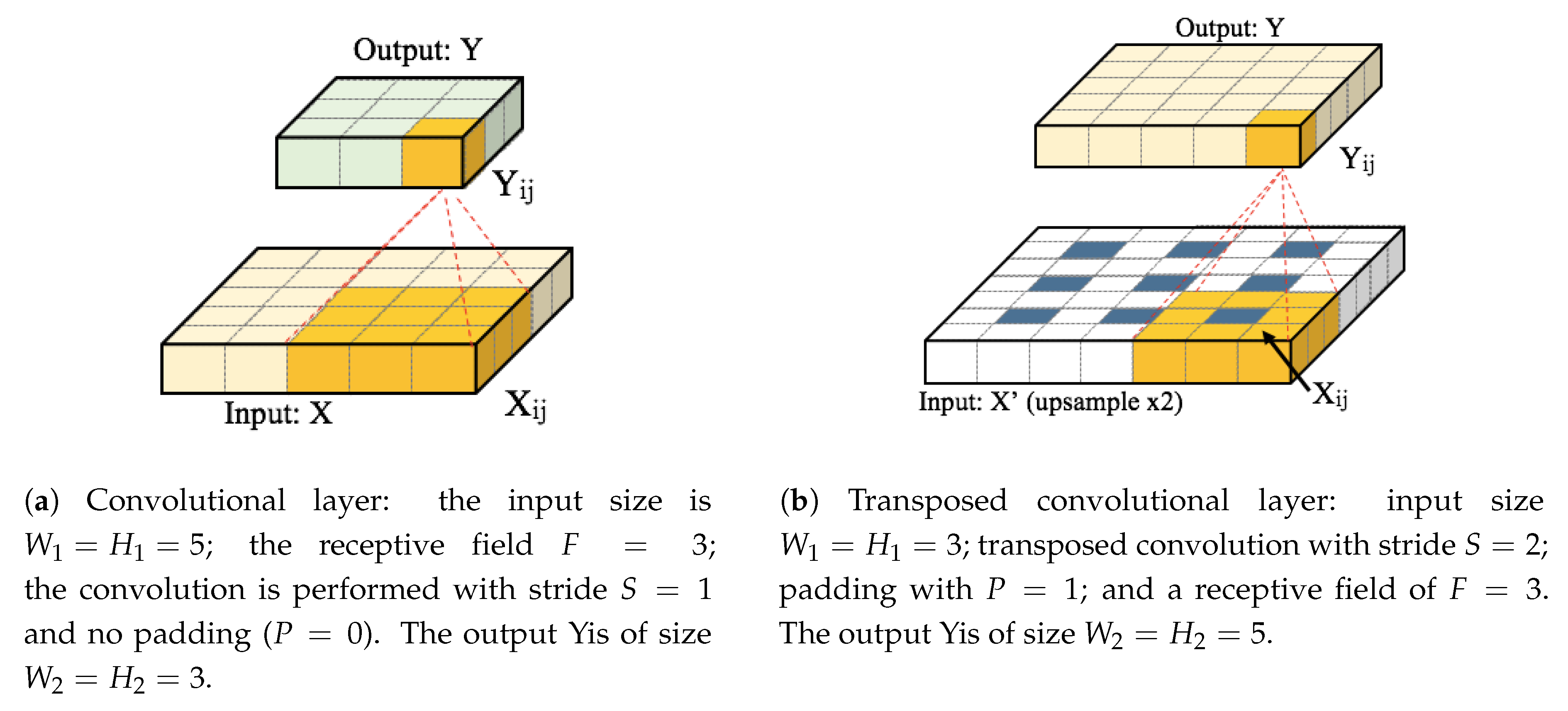
2.1.1. Convolutional Layer

The convolutional layer is the core of CNNs. It can be seen as a bank of simple filters with learnable parameters. As illustrated in Figure 1a, the layer takes the input X of size W 1 × H 1 × C 1 and convolves it with the filter bank by sliding of stride S and padding the border with P units. The result of this operation is an output volume Y with size W 2 × H 2 × C 2 . Equation (1) formulates the calculation of the output at spatial position ( i , j ) as:
Y i j = W × N i j + b
where ( W , b ) are the learnable parameters (weights and bias) of the layer, N i j is the corresponding receptive field (or a window surrounding X i j ) and W × N denotes the dot product between W and N.
The spatial dimensions of the output of the convolutional layer are given by W 2 = ( W 1 F + 2 P ) / S + 1 , H 2 = ( H 1 F + 2 P ) / S + 1 where F is the size of the receptive field, which also corresponds to the spatial size of the filters. In general, each filter can take different widths and heights, but conventionally, most CNN architectures employ filters with square masks of dimension F. In our work, we consider only filters with square masks.
Neurons in the output volume Y can be considered as filters of size F × F × C 1 . Intuitively, each neuron looks for a specific pattern in the input volume X. Since we want to look for the same pattern across all spatial locations in the input volume, the learnable weights and bias for all neurons in a channel of Y are shared. This is often called parameter sharing, and by doing this, the output volume Y consists of the values obtained when applying C 2 filters on the input volume X. The parameter sharing also reduces the number of weights of a convolutional layer to C 2 × F × F × C 1 , which is much smaller than that of a fully-connected layer. This helps mitigate the problem of overfitting in neural network training.

2.1.2. Transposed Convolutional Layer

The transposed convolutional layer, also known as the deconvolution layer, was first introduced in [23]. An example of the transposed convolutional layer is shown in Figure 1b. This layer is commonly employed for up-sampling operations in CNNs [18]. As shown in Figure 1b, the input is first up-sampled by a factor of stride S and padded spatially with P units if necessary. After that, convolution is applied to the up-sampled input with a filter bank that has a receptive field of size F. Transposed convolution can be thought of as the inverse operation of convolution. Filter parameters can be set to follow conventional bilinear interpolation [18] or can be set to be learned.

2.1.3. Non-Linear Function Layer

The convolution layer is often followed by a non-linear function layer, also called an activation function. The role of this layer is similar to that of a fully-connected layer in traditional neural networks. This layer introduces non-linearity in the network and enables the network to express a more complex function. Common activation functions include the Sigmoid function, the Tanh function, the rectified linear unit (ReLU) function [24] and the leaky ReLU function [25]. Among these functions, the ReLU function f ( x ) = m a x ( 0 , x ) is the most commonly used in deep-learning research. In our proposed network design, we also select ReLU as the activation function due to its efficiency and light computational complexity.

2.1.4. Spatial Pooling Layer

The spatial pooling layer is used to spatially reduce the size of the input volume [26]. A small filter (typical size: 2 × 2 or 3 × 3) is used to slide through the volume to carry out a simple spatial pooling function. Common pooling functions include max, mean and sum functions. One notes that it is also possible to use the convolutional layer to replace the pooling layer [27]. However, this practice does not necessarily lead to performance benefits and would cost extra memory and training effort [28]. Among the common pooling functions, the max function is most commonly used in the literature. We also employ the max pooling function in our network design.

2.2. CNN Architectures for Semantic Segmentation of Remote Sensing Images

In the literature, there are two basic approaches for semantic segmentation, namely patch-based and pixel-based approaches. In this section, we present an analysis of both categories.

2.2.1. Patch-Based Methods

Patch-based approaches infer the label of each pixel independently based on its small surrounding region. In these approaches, a classifier is designed and trained to predict a single label from a small image patch. In the inference phase, a sliding window is used to extract patches around all pixels in the input image, which are subsequently forwarded through the classifier to get the target labels [29]. Several techniques have been proposed to achieve high performance with patch-based approaches. For instance, replacing the fully-connected layer in the network with convolutional layers can lead to more efficient algorithms by avoiding overlapping computations [22,29]. Multi-scale inference and recurrent refinements can also lead to performance gains [30,31]. Nevertheless, patch-based approaches are often outperformed by pixel-based methods in remote sensing semantic segmentation tasks [21,22]. As a result, in this work, we put more emphasis on the pixel-based approach and follow such a paradigm in our design.

2.2.2. Pixel-Based Methods

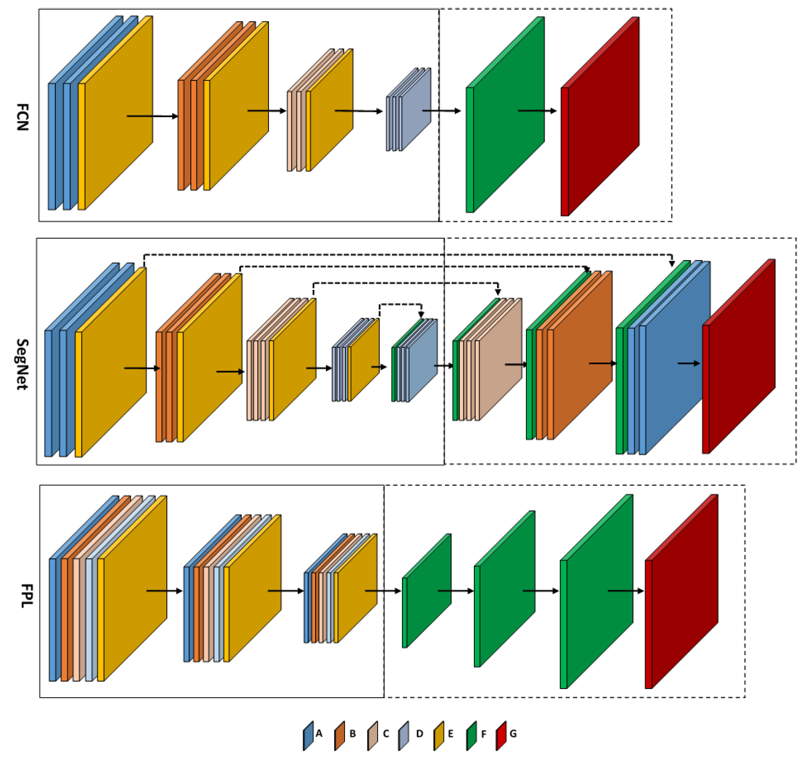
Unlike patch-based approaches, pixel-wise methods infer the labels for all of the pixels in the input image at the same time. One of the first CNN architectures for pixel-wise semantic segmentation is the fully-convolutional network (FCN) method introduced by Long et al. in [18]. In this method, a transposed convolutional layer is employed to perform up-sampling. This operation is essential in order to produce outputs of the same spatial dimensions as the inputs.
The FCN architecture was recently employed for semantic segmentation of remote sensing images in [21]. Its architecture, shown in Figure 2, can be divided into two parts, namely encoding and decoding. The latter is depicted within the dotted-line box in the figure. The encoding part follows the same architecture as the VGG-net of [32], which is one of the most powerful architectures for image classification. In Figure 2, the layers A, B, C and D are convolutional layers; their configurations (width, height, depth) are shown in Table 1. Each convolutional layer is followed by a batch normalization layer [33] and ReLU activation function. The final convolutional layer of Type D is followed by a 1 × 1 convolution, producing an output with scores for each classes. Layer E is a max pooling layer with size F = 2 and stride S = 2 . It performs a down-sampling operation with a factor of two in each dimension. Layer F is a transposed convolutional layer, with filter size F = 16 and stride number S = 8 . It up-samples the scores to original image size. It should be noted that after each pooling layer, the number of filters in the next convolutional layers is doubled to compensate the spatial information loss. To train the network, a median frequency weighted softmax loss layer (Layer G) is appended after the last transposed convolutional layer.
In this FCN design [21], the transposed convolutional layer up-samples the score by a large factor of eight in each dimension. This incurs the risk of introducing classification ambiguities in the up-sampled result. To mitigate this problem, in [22], Volpi et al. proposed to use multiple transposed convolutional layers to progressively up-sample the classification scores. This design is named full patch labeling by learned up-sampling (FPL) [22], its architecture being depicted in Figure 2. Similar to FCN, the FPL network also consists of encoding and decoding modules. However, unlike the FCN design, which incorporate unique layer types in each convolutional module, in FPL, the convolutional modules consist of all four different convolutional layer types, A, B, C and D (see Figure 2). Their configurations are shown in Table 1. Each convolutional module is followed by a max pooling layer, batch normalization layer and leaky ReLU activation. In Figure 2, the pooling and leaky ReLU layers in FPL are grouped together and shown as Layer E. In the decoding stage, three transposed convolutional layers (Type F) are stacked sequentially to spatially up-sample the score to the input image size. They all have an up-sampling factor of two in each spatial dimension. For training, a softmax loss layer (Type G) is appended at the end of the network. The FCL design aims at improving the output classification result by allowing the transpose convolutional layers to learn to recover the fine spatial details. Semantic segmentation results on the Vaihingen dataset reported in [22] show that the FPL network outperforms the FCN design in terms of overall accuracy.
Besides using the transposed convolutional layer for up-sampling in the decoding stage, Vijay et al. proposed to use unpooling in SegNet [19] for pixel-wise segmentation tasks. The encoder part of SegNet (see Figure 2) consists of consecutive convolution layers with uniform 3 × 3 size filters, followed by ReLU activations and pooling layers. The detailed network parameter settings are given in Table 1. The decoder uses pooling indices computed in the max-pooling step of the corresponding encoder to perform non-linear up-sampling (via an unpooling Layer F), followed by mirror-structured convolution layers to produce the pixel-wise full size label map. Finally, a loss Layer G is attached for network training. The SegNet design aims at preserving the essential spatial information by remembering the pooling indices in the encoding part, which produces state-of-the-art accuracy in generic image segmentation tasks.
Both FCN and FPL architectures suffer from two problems, namely the insufficient spatial information in the decoding stage and the lack of contextual information. Due to the first problem, the FCN and FPL networks often mislabel small objects like cars and produce poor results around object boundaries. Due to the second problem, the lack of contextual information makes it difficult for these architectures to correctly infer classes in difficult areas, such as shadow regions projected by high-altitude buildings and trees.
SegNet effectively mitigates the insufficient spatial information problem by adopting unpooling layers in the decoder part, but it may also suffer from the lack of contextual information. Furthermore, as shown in Table 2, SegNet has three-times more trainable weights than FCN and FPL, making the training phase much more difficult. In this paper, we propose a novel network architecture to address these issues.

3. Proposed CNN Architecture for Semantic Segmentation

In this section, we present our novel CNN architecture for semantic segmentation of remote sensing images. The section details first the network design, followed by the training and inference strategies, our post-processing technique and a brief analysis.

3.1. Proposed Hourglass-Shaped Convolutional Neural Network

Our CNN follows a pixel-wise design paradigm, which has been shown to produce state-of-the-art results in semantic segmentation. However, as mentioned in Section 2.2, existing pixel-wise network architectures suffer from the spatial-information loss problem. To overcome this problem, we propose a novel hourglass-shaped network (HSN) architecture. Our HSN design was partially inspired from recent important works in deep learning research [17,34,35].

3.1.1. Network Design

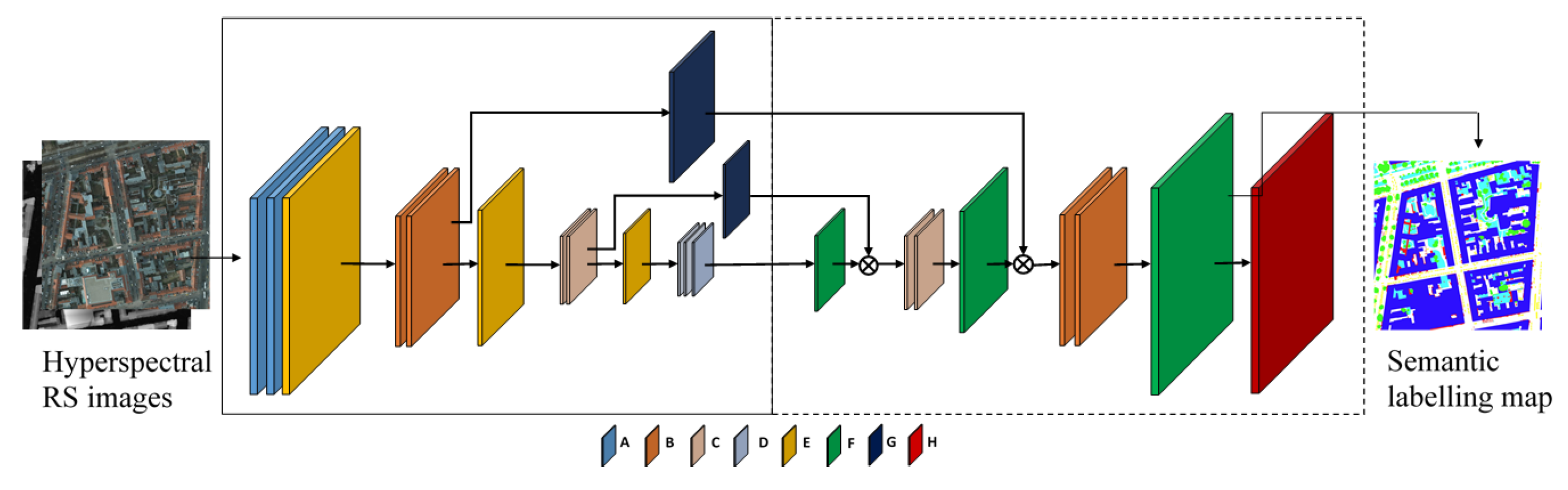
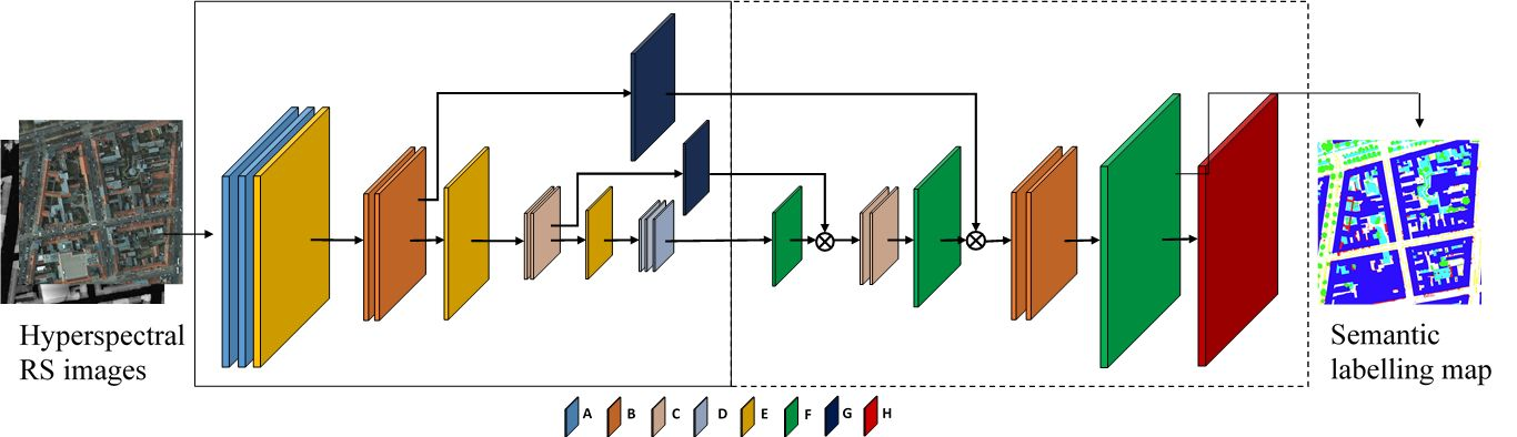
Similar to FCN and FPL, our HSN architecture follows the generic encoder-decoder paradigm, as illustrated in Figure 3. In the figure, the encoder and decoder parts are delimited by continuous and dashed rectangular boxes, respectively. As mentioned in Section 2.2, one key point is to use transposed convolutional layers to progressively up-sample the pixels’ class scores to the original spatial resolution of the input image. However, novel components are brought in the network design. Inspired by the hourglass-shaped network introduced for human pose estimation [36] and image depth estimation [35], we propose a network that features (i) multi-scale inference by using inception modules [34] replacing simple convolutional layers and (ii) forwarding information from the encoding layers directly to decoding ones by skip connections.
The network starts with two layers of A and two layers of B, which are common convolutional layers with filter size F = 3 
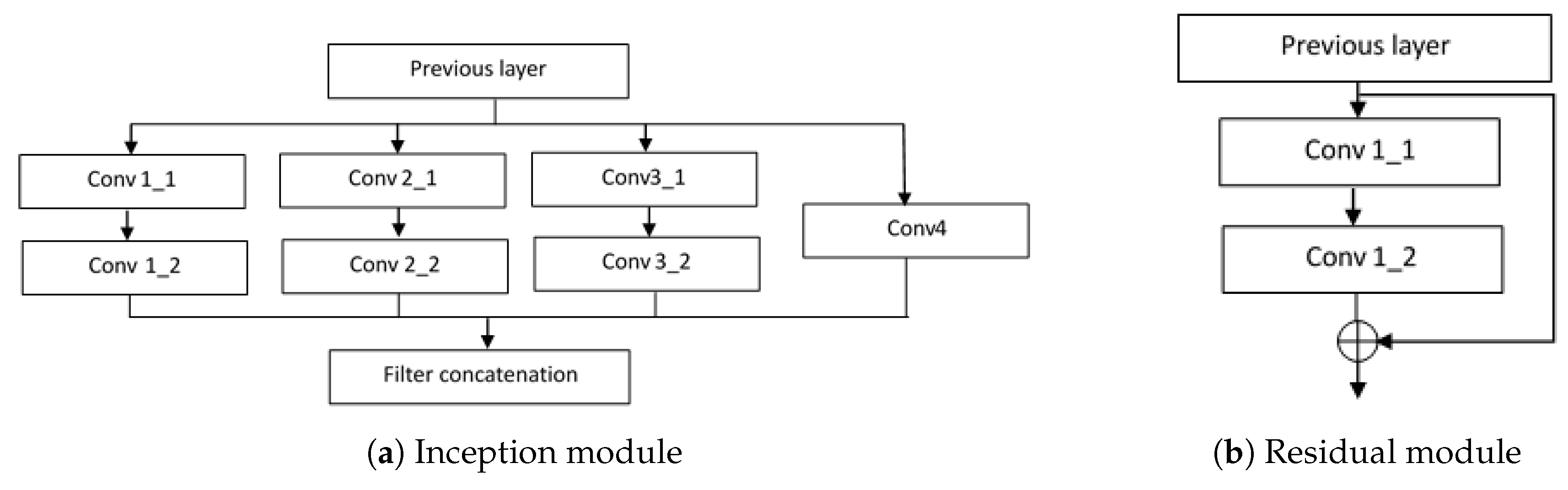
. The number of filters are 64 and 128 for Layers A and B, respectively. Each convolution layer is followed by a batch normalization layer and ReLU activation. Layer E is a max pooling layer, with a down-sampling factor of two. Layers C and D are composed of inception modules, as shown in Figure 4a. The configurations of convolutional layers in the inception modules are shown in Table 3. As can be seen from the table, filters of different sizes are assembled in one inception module to enable multi-scale inference through the network.
In the encoding part, after the second Layer B and after Layer C, two skip branches are made with Layer G, forwarding information directly to the corresponding layers in the decoding part. Layer G is a residual module inspired by ResNet [17]. The residual module is shown in Figure 4b, where c o n v 1 _ 1 is a bank of 128 filters with size 1 × 1, and c o n v 1 _ 2 is another bank of 128 filters with size 3 × 3 . The input of the module is directly element-wise added to the output of c o n v 1 _ 2 . It is worth mentioning that, due to the use of filters with size 1 × 1, the number of trainable weights for the whole network is significantly reduced. As shown in Table 2, the total number of trainable weights of HSN is comparable to that of FPL and nearly three-times less than that of SegNet.
In the decoding part, Layer F serves as the transposed convolutional layer, with the same up-sampling factor of two. After the first and second up-sampling, data directly forwarded from the encoding part are concatenated with the outputs of the transposed convolutional layers. Finally, Layer H, which is a weighted softmax layer, is used in the training phase of the network.

3.1.2. Median Frequency Balancing

We train our network using the cross-entropy loss function, which is summed over all of the pixels. Nevertheless, the ordinary cross-entropy loss can be heavily affected by the imbalance of the class distribution when applied to high-resolution remote sensing data. To address this problem, the loss for each pixel is weighted based on the median frequency balancing [21,37] technique. The weighted loss for a pixel i is calculated as:
L ( i ) = c = 1 C [ y i = c ] l o g ( p ^ i ( c ) ) × w c
where y i is the ground-truth class of pixel i, w c is the weight for class c, f c is the pixel frequency of the class and:
w c = m e d i a n ( f c | c C ) f c

3.2. Training Strategy

We train the network to optimize the weighted cross-entropy loss function using mini-batch stochastic gradient descent (SGD) with momentum [38]. The parameters are initialized following [39]. The learning rate is set to step down 10-times from 1 × 10 5 every 50 epochs, with momentum set to 0.99. The batch size is set to fit the memory. Data augmentation is carried out to mitigate overfitting. The image patches are extracted with size 256 × 256 with 50% of overlap and flipped horizontally and vertically. Each patch is also rotated at 90 degree intervals. In total, this produces eight augmentations for each overlapping patch. We train our network from scratch until the loss converges. Batch normalization is employed, similar to existing network architectures. The training and testing processes are performed on a desktop machine equipped with Nvidia GeForce Titan X (12 Gb vRAM).

3.3. Overlap Inference

In the inference stage, due to the memory limit, the input high-resolution images can be sliced into small non-overlapping patches to feed-in the network. However, this may cause inconsistent segmentation across the patch borders and hence result in degraded accuracy.
To address such boundary effects, overlap inference is employed whereby input images are split into overlapped patches. At the output of the network, the class scores in overlapped areas are averaged. We experimentally justify the benefit of this strategy compared to non-overlapping inference in Section 4.

3.4. Post-Processing with Weighted Belief Propagation

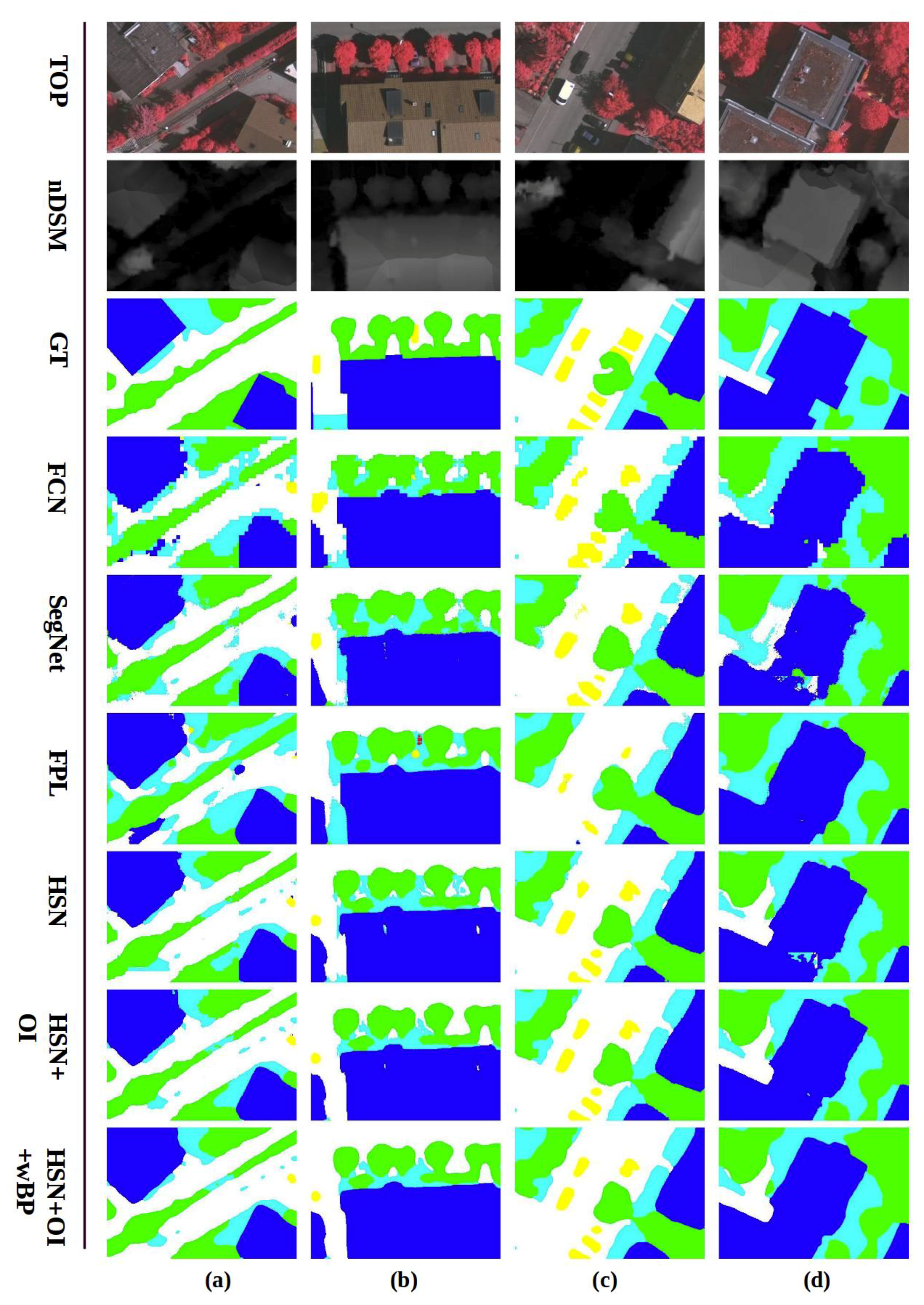
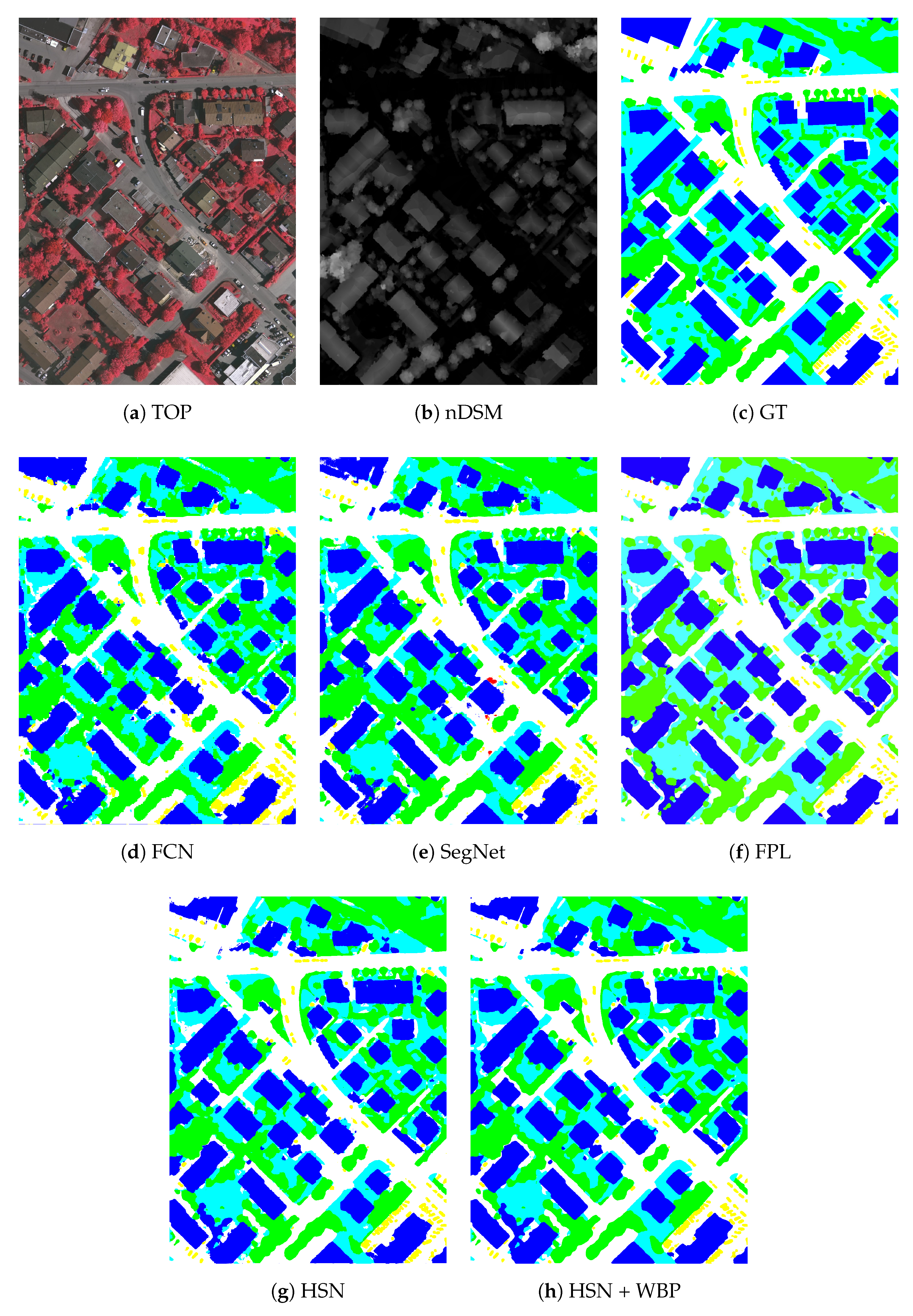
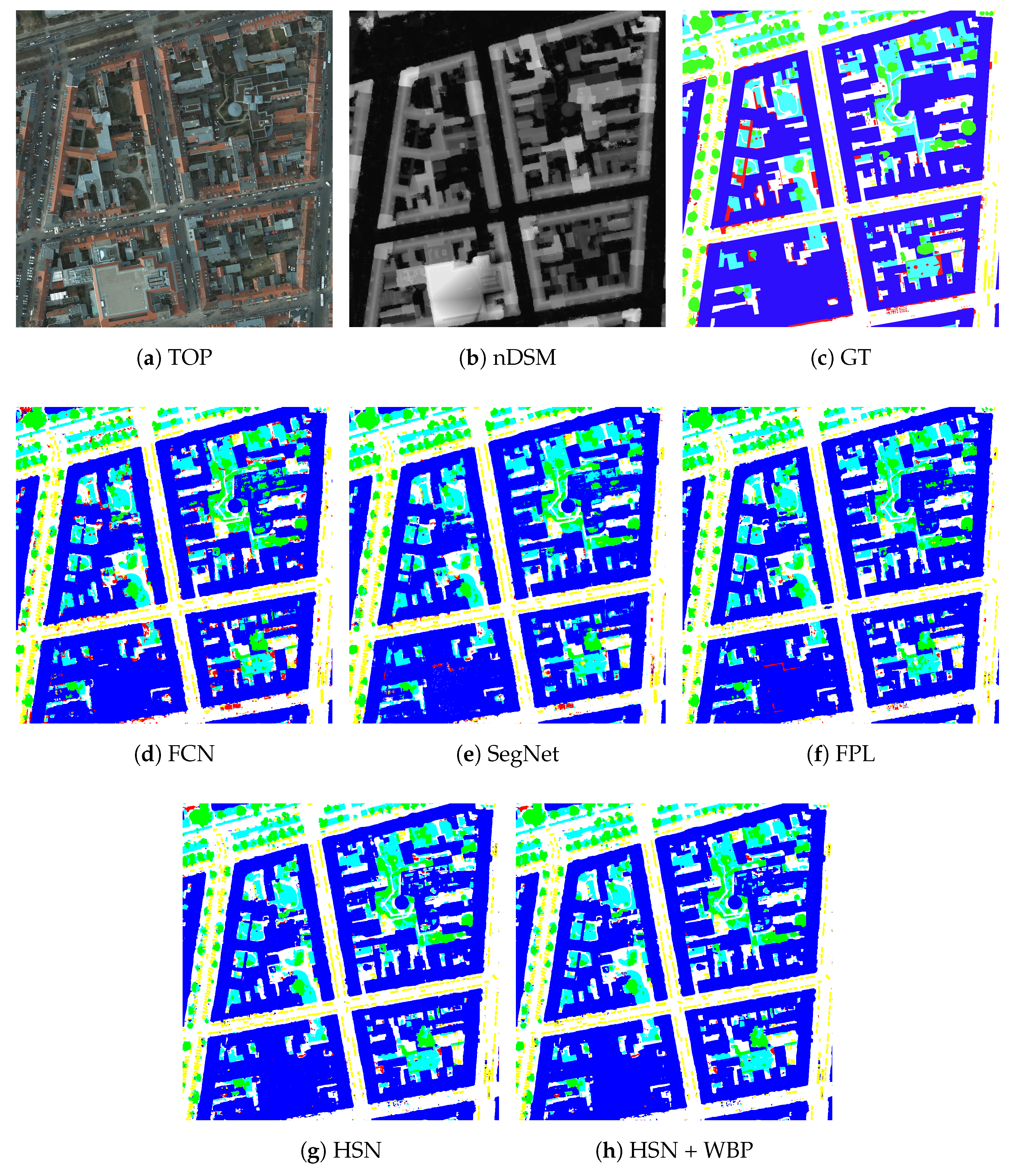
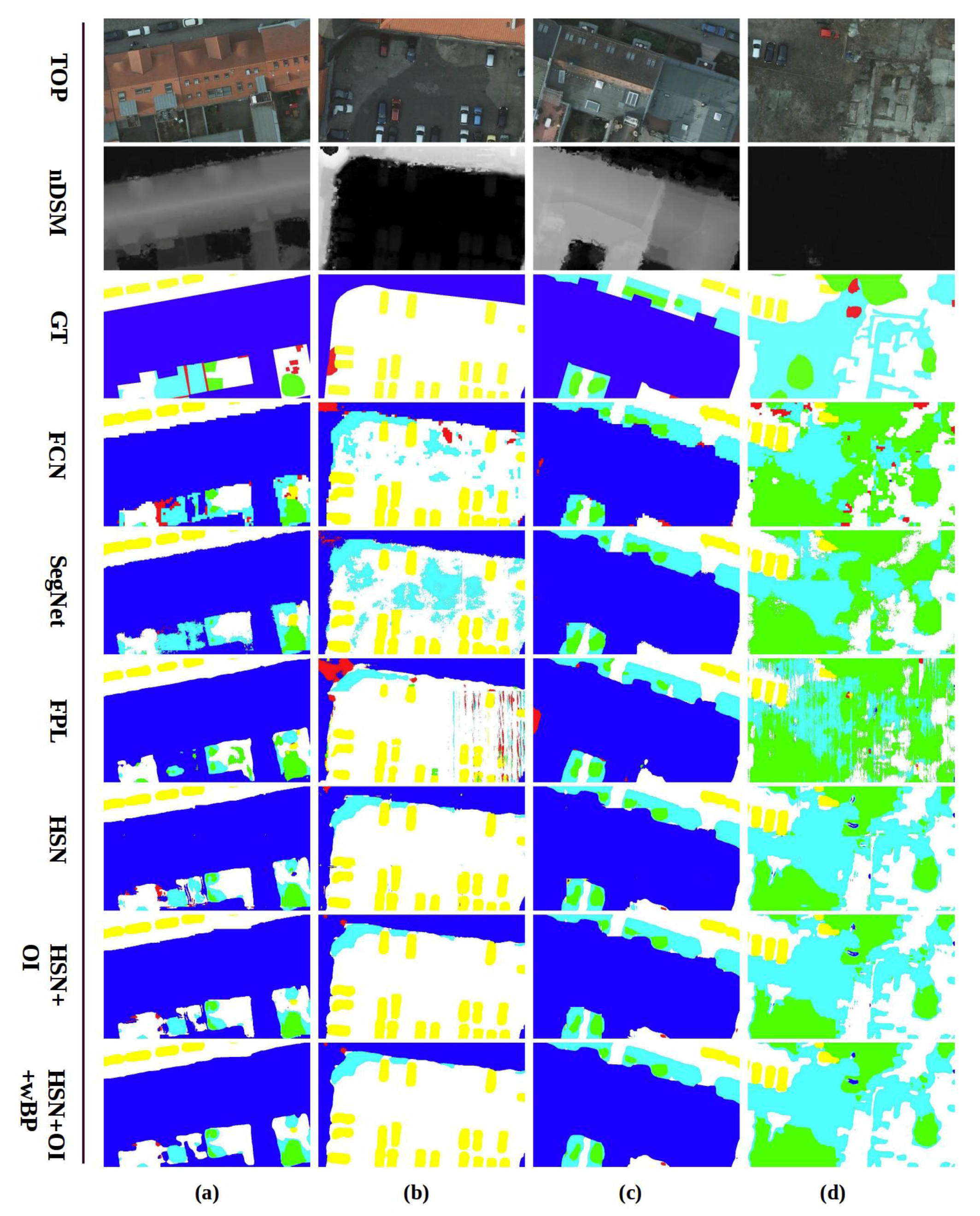
Semantic segmentation for high-resolution remote sensing imagery often requires accurate and visually clear results to serve further automatic processing or manual investigations. However, the raw network output may feature zigzag segment borders and incorrect blobs. Some examples are shown in Figure 5, Figure 6 and Figure 7. To address this problem, we propose to use weighted belief propagation for post-processing the raw network outputs.
In the proposed HSN architecture, the semantic label for a pixel at an arbitrary position i is determined as L ( i ) = arg max c f i ( c ) , where f i ( c ) denotes the score of class c for pixel i. This corresponds to the top one class prediction, i.e., the class label with the highest score. Similarly, the top two prediction for any arbitrary pixel is defined as the set of class labels when taking the best two scores for that pixel. We experimentally observed that the top two prediction accuracy for the validation data is around 97% on the Vaihingen dataset. This shows that most of the time, the right labels lie in the top two scores determined by the network.
Let d i = f i ( c 1 ) f i ( c 2 ) , in which f i ( c 1 ) and f i ( c 2 ) refer to the top two scores, i.e., the highest and second highest class scores for pixel i, respectively. Intuitively, for a trained network, the higher d i is, the more confident the network is about its prediction. Therefore, d i can be thought of as the confidence of the output at position i.
We consider post-processing as a pixel labeling problem and formulate a Markov random field (MRF) model to solve it. A node i in our MRF model corresponds to a pixel in the original image I, which is directly connected to its four spatial neighbors N i . y i denotes the class label assigned to node i. We find the optimal labels for the whole image by minimizing the following energy function:
E = i I E d ( y i ) + i , j I E s ( y i , y j )
where E d , defined in Equation (5), refers to the data energy term describing how confident the estimated label y i is; E s is the smoothness energy defined in Equation (6), which penalizes the inconsistency between node i and its neighbors N i :
E d ( y i ) = exp f i ( y i ) Σ j C exp f i ( j )
E s ( y i , y j ) = v 2 exp ( 1 δ ( y i y j ) T )
where v 2 and T are hyper-parameters, which are set empirically, and δ ( x ) is the Dirac delta function. We employ the weighted belief propagation algorithm (WBP) [40,41] to iteratively minimize the energy function E. At each iteration, the update rule of WBP is expressed by Equations (7) and (8) below:
m i j ( y j ) = w i y i C E s ( y i , y j ) E d ( y i ) y k N i \ y j m k i ( y i )
b i ( y i ) = E d ( y i ) y k N ( y i ) m k i ( y i )
in which m i j ( y j ) is the message passed from node i to node j; w i is the weight for node i, which is set to its confidence value d i ; b i ( y i ) is the belief, which represent how confident the node i is to take label y i .
The messages are updated until convergence. The final label y i ^ at node i is determined by y i ^ = arg max y i b i ( y i ) .

4. Experimental Results

We carried out extensive experiments to assess the effectiveness of our proposed HSN architecture. We employed two well-known datasets in the semantic segmentation literature, namely the Vaihingen and Postdam datasets [42,43]. In this section, we describe our experimental settings and report quantitative and qualitative results. We evaluate the benefits of each of the components in our proposed method and compare our results to those of the FCN [21], SegNet [19] and FPL [22] networks. It should be noted that, as Kampffmeyer et al. [21] do not provide their trained model, we strictly followed their network design and training configuration to reproduce their results. For FPL [22], we have carried out experiments using the original FPL network, which was trained on the Vainhingen and Potsdam datasets and was publicly made available by its authors. Concerning SegNet, it was originally devised and tested on generic image datasets; to produce the results, we employed the network provided by the authors and trained it from scratch using the aforementioned remote sensing datasets.

4.1. Datasets

4.1.1. Vaihingen Dataset

The Vaihingen dataset consists of thirty three very high-resolution true orthophoto (TOP) tiles and their corresponding digital surface models (DSMs). Normalized DSMs (nDSMs), which limit the effects of varying ground height, are also provided by Gerke et al. [44]. The tiles have a spatial resolution of 2949 × 2064, with the number of pixels varying from three million to 10 million pixels. Each TOP image is composed of three channels: near-infrared (NIR), red (R) and green (G), with a spatial resolution of 9 cm. Ground-truth labeled images for sixteen out of thirty three tiles were provided by ISPRS. In these images, pixels are labeled as one of the six classes: impervious surfaces, building, low vegetation, tree, car and clutter/background. Examples of the TOP, nDSMs and the corresponding ground truth images are shown in Figure 6.
Following the same training and testing procedures as set by FCN [21] and FPL [22], we used the sixteen annotated tiles in our experiments. Eleven tiles (areas: 1, 3, 5, 7, 13, 17, 21, 23, 26, 32, 37) were selected for training, while the other five tiles (areas: 11, 15, 28, 30, 34) were reserved for testing.

4.1.2. Potsdam Dataset

The Potsdam 2D segmentation dataset includes 38 tiles of high resolution remote sensing images. All of them feature a spatial resolution of 5 cm and have a uniform resolution of 6000 × 6000 pixels. For each tile, five channels are provided, namely near-infrared (NIR), red (R), green (G), blue (B), together with the digital surface models (DSMs). The normalized DSMs (nDSMs) are also made available by Gerke et al. [44]. Twenty four tiles are provided with ground-truth pixel labels, using the same six classes as in the Vaihingen dataset. In our experiments, we employed all five channels, namely NIR-R-G-B and the nDSMs as inputs to the networks. Following the practice in [22], six tiles (02_12, 03_12, 04_12, 05_12, 06_12, 07_12) were selected as testing set, while the other eighteen among the annotated tiles were used for training.

4.2. Evaluation Metrics

To compare our results with the state-of-the-art, we strictly use the same evaluation metrics as in [20,21,22,42]. Besides the conventional pixel-wise ground truth, in both datasets, border-eroded ground-truth label images are also available. In these images, borders between classes are eroded with a disk radius of three pixels [42,43]. We report our results for both ground-truth versions. All pixels are considered for the conventional pixel-wise ground-truth version, while for the eroded version, border pixels are not accounted for.
We evaluate the performance of the different methods based on three criteria, namely, per-class F-score, overall accuracy and average F-score. The F-score is defined as:
F-score = 2 × p r e c i s i o n × r e c a l l ( p r e c i s i o n + r e c a l l )
The overall accuracy is the total number of correctly-labeled pixels divided by the total number of pixels. In the Vaihingen dataset, the clutter class only accounts for an extremely small number of pixels. As a result, following the common practice [20,21,22], we neglect the clutter class when reporting the result for this dataset. For the Potsdam dataset, we report the results on all six classes.
Confusion matrices are also provided in the Appendix A for the experiments based on the eroded ground-truth for both datasets. We averaged the values in the confusions matrices across all tested tiles and reported the results for the proposed HSN and the reference techniques.
It is also worth mentioning that ambiguities and mislabeling exist in the provided dataset [20]. There are also some errors for the input normalized DSM [44].

4.3. Overlap Inference Size

Table 4 reports the experimental results obtained on the Vaihingen dataset with four different overlap inference sizes, namely 0%, 25%, 50% and 75%. The results are organized into two groups, corresponding to the two ground-truth versions used in the evaluation: the eroded version (indicated by erGT) and the original version (denoted by GT). It can be observed that the classification performance improves when increasing the overlap size. Overlap inference solves potential border effects at tile boundaries and returns the final classification results by performing a multi-hypothesis prediction of pixel classes instead of single-hypothesis prediction performed in the non-overlapped case. Further increasing the overlap size beyond 75% does not lead to significant improvements in classification performance.

4.4. Skip Connections and Inception Modules

We further analyze the influence on the performance of our key design components by performing the following experiments: firstly, we remove all skip connections from HSN to study the possible benefit brought by the residual modules; secondly, we keep the residual modules, but replace all of the inception layers with normal convolutional layers to check the influence of inception modules. The results are reported in Table 5 for the first and second set of experiments denoted as HSN-NS (no skip) and HSN-NI (no inception), respectively.
From Table 5, it can be observed that both residual and inception modules critically contribute in the HSN design. When removing the residual module, corresponding to the HSN-NS results, a sharp drop in the F-score of the car class is observed. Replacing the inception module with normal convolutional layers leads to a nearly 4% drop in overall accuracy when compared to the eroded ground truth (see NSN-NI results in Table 5).
Visually, from Figure 5, we can observe that the segmentation result of HSN is more coherent compared to the results of HSN-NI and HSN-NS. For instance, when removing the inception layers, there are mislabeled artifacts on the bottom of the image or on the building on the right up corner, the result of HSN being more clean. When removing skip connections, the same effect can also be observed on the road segmentation in the middle bottom of the image.

4.5. Performance Evaluations

In this section, we report extensive experimental results obtained with the proposed HSN and other networks, namely FCN [21], SegNet [19] and FPL [22], which serve as baselines. The HSN applied in this section includes both the inception layers and residual modules. Overlap inference with 75% overlapping size and post-processing with weighted belief propagation are also integrated to demonstrate their effectiveness.

4.5.1. Vaihingen Dataset

Numerical results

Table 6 reports the experimental results obtained in the Vaihingen dataset. The results are organized in the same manner as in Table 4. From the table, it can be observed that the proposed HSN network outperforms the other networks in terms of overall performance. For all classes, except the buildings class, HSN reaches a better performance. Especially in the car class category, HSN significantly outperforms FCN and FPL by more than 10%, and outperforms SegNet by around 5%. Further, by consulting the confusion matrix provided in Table A1, we find that the car class is often mislabeled as impervious surface; trees and low vegetation are also easily confused by the network. It can also be observed that the augmentation in HSN’s average F-score is mainly due to the improvement in the car class. Overlap inference (OI) systematically improves the prediction accuracy for each class, bringing up the average F-score to 87.52%. This proves the effectiveness of overlap inference. Post-processing with WBP slightly improves the overall accuracy to 88.82%.
In case border pixels are taken into account (GT), all of the networks perform worse than in the case in which the border pixels are ignored (erGT). This is due to the ambiguities around object boundaries. In case the original GT is used as the reference, post-processing with WBP shows minor performance degradation in some classes, such as car, impervious surface and buildings; yet, the overall accuracy is not affected, and the visual results are improved, as we will see next.
In both cases, all of the networks have high accuracy on the building class thanks to the provided normalized DSM.
Table 7 shows the average inference time per image on the test dataset (five images in total). As the proposed HSN employs a more complex architecture, it takes 15.87 s (3.17 s per image) to finish inference on the five test images with an average size of 2563 × 1810 pixels. While HSN gives the best overall accuracy, it almost doubles the inference time when compared to SegNet, which shows the trade-off between performance and time efficiency. We also note that in [22], the authors of FPL report an average time of 6.2 seconds for inference on the same dataset; this longer inference time for FPL may be caused by the implementation of the network (FCN, SegNet and the proposed HSN are implemented based on the Caffe framework, while FPL is provided in MatConvNet).

Qualitative Results

As semantic segmentation often serves other remote sensing applications, visual output quality plays also an important role besides pixel-wise accuracy. For a visual demonstration, Figure 6 shows the labeling results for a complete tile, while Figure 7 zooms into certain areas showing the details of the outputs.
From the figures, it can be seen that the shadows from tall buildings or trees pose great difficulties for semantic labeling. For example, in Figure 7d, we can observe that the road on the left of the building is completely shadowed by the buildings in the middle. In this case, both FCN and FPL methods label this part as the low vegetation class. SegNet managed to detect the road existence, but the segmentation accuracy is quite low. The proposed HSN managed to roughly tag the road. We argue that the inception module design may contribute to this advantage, since using filters of different sizes in one layer allows the network to access multi-scale receptive areas. This aids the network to acquire richer contextual information, which is essential to predict pixels in occluded or shadowed regions.
The car class is quite difficult to deal with, since in the images, cars have various colors leading to a large intra-class difference, whereas dark colored cars are quite similar to the road under shadows (see Figure 7c, for example). FPL fails to label most of the cars, as shown in Figure 7c, due to shadows. HSN successfully detects most of the cars, and the pixel-wise labeling is clear and precise compared to the ground truth. One notes that, since the cars are rather small objects compared to the other classes like buildings, they take fewer pixels in total which in general leads to the class imbalance problem. Median frequency balancing puts a larger weight on the loss for the car class, compensating for its lower occurrence rate in the training phase.
Due to limitations in GPU memory, the high resolution remote sensing image is often split into small-sized patches to perform network inference. As explained in Section 3.3, this practice may possibly introduce erroneous artifacts in the result. For example, in Figure 7d, in the center of the building, both the raw results of HSN and SegNet show artifacts by mislabeling part of the building as low vegetation. However, overlap inference effectively solves this problem by performing multi-hypothesis prediction, whereby the class for each pixel is identified in several overlapping patches. This always leads to more robust results compared to single-hypothesis prediction performed when using non-overlapping inference. Moreover, each patch provides different contextual information for classification, which again contributes to improved classification accuracy compared to the raw HSN.
The provided normalized DSMs help the segmentation of the buildings and trees, as for all of the results, the building segmentation is coherent with the ground-truth. FCN results show obvious zigzags on the class boundaries, while HSN produces sharper and more accurate boundaries (for example, see in Figure 7d the building segment boundaries). Both the hourglass design and post-processing with WBP contribute to this improvement. Thanks to the skip connections with residual modules, information from the encoding stage can be passed directly to the decoding stage. In the early layers of encoding, the data maintain high spatial resolution. Hence, when being fed forward directly to the decoding stage, this information helps with reducing the spatial ambiguities. The WBP in the post-processing stage encourages continuity by propagating the class confidences across pixels throughout the output, hence making the results smoother and correcting small erroneous blobs.

4.5.2. Potsdam Dataset

Numerical Results

Table 8 shows experimental results for the Potsdam dataset. The results are organized similar to those reported in Table 6 for the Vaihengen dataset. The F-score for each class and overall performance are shown respectively for erGT and GT.
From the table, it can be seen that the raw HSN outperforms FCN [21], SegNet [19] and FPL [22] in terms of accuracy for all but the clutter class. In terms of overall accuracy, the proposed HSN outperforms the reference techniques, but SegNet outperform HSN in terms of average F-score and F-score in the clutter class. Overlap inference and WBP help further improve the accuracy, leading to higher overall performance compared to the other three network architectures.
In the Potsdam dataset, the clutter class accounts for a higher percentage of pixels than in the Vaihingen dataset, making it non-negligible. Nevertheless, various types of objects like pedestrian, fence, playground, constructions sets, etc., are all labeled as clutter. This high intra-class variance makes it challenging for the networks to correctly classify clutter pixels (see Figure 8 and Figure 9). As can been seen from Table 8, all of the networks, except FCN and SegNet, give a F-score with values below 20 in the clutter class; Table A2 also shows that the clutter class is often mislabeled as impervious surface and buildings. In contrast, for the building class, all networks reach a high accuracy of more than 95%. We claim that this saturation is due to the provided nDSM channel as the height of the surface gives a strong indication of buildings when combined with other channels’ information.
Generally, all of the networks perform better in the Potsdam dataset compared to the Vaihingen dataset, since the images in the Potsdam dataset have a higher spatial resolution (of 5 cm) and an extra blue channel is available. In addition, more data are available in the Potsdam dataset, which leads to better training of the networks.

Qualitative Results

Full tile prediction results from different networks are depicted in Figure 8. Certain clips are selected and shown in Figure 9 to illustrate and analyze the performance of the networks.
The buildings are always well labeled thanks to the aid provided by the nDSM channel, as shown in Figure 8. However, in Figure 9c, the building roofs show a complex pattern, which leads to partial mislabeling for FCN and FPL. For HSN, the inception module mitigates this problem, as it provides the network with multi-scale contextual information. The same effect can be also observed in Figure 9b. The label maps from both SegNet and FCN are quite noisy, with low vegetation class scattered among the road. FPL provides better results, but still with some mislabeling, like part of the small car in the center is labeled as tree. HSN provides a more accurate and visually improved result.
FPL infers pixel labels using a patch with a smaller size of 64 × 64 compared to the other networks, which may lead to a restricted receptive area. As shown in Figure 9a, the court yard behind the buildings is mislabeled as buildings, while the other two networks label the yard correctly. As shown in Figure 9, for all three network structures, the clutter areas are hard to accurately label; from the same figure, we can also observe smoother borders in the class map obtained with the proposed networks.
It is also worth mentioning that, in the Potsdam dataset, most trees are not covered with leaves, which causes difficulties for the networks to detect and segment them accurately. As shown in Figure 9d, trees can be barely distinguished from the surrounding grasses. All reference networks mislabeled nearly half a part of the tree class, but HSN can still correctly distinguish the tree class from the low vegetation.

5. Discussion

The experimental results in Section 4 prove that state-of-the-art performance on well-known remote sensing datasets is achieved with our approach. On the Vaihingen dataset, the proposed approach outperforms reference methods by substantial margins in terms of both average F-score and overall accuracy. On the Potsdam dataset, it is marginally worse than SegNet in term of average F-score, but noticeably better in terms of overall accuracy. Besides, the proposed approach systematically performs better than FCN and FPL on this dataset. In addition, this high performance is achieved with relatively low complexity. The number of trainable parameters in our network is just slightly higher than that of FPL while being far lower than those of FCN and especially SegNet, which has three-times more parameters than the proposed network.
We argue that the effectiveness of the propose approach comes from the highly complementary characteristics of different components in the architecture. Firstly, the use of skip connection with residual modules helps with transferring spatial information from the encoder directly to the decoder, improving the segmentation around object borders. Secondly, the use of inception provides the decoder with richer contextual information. This helps the network to label difficult areas such as roads, which are shadowed and which can be correctly inferred if enough surrounding contexts are available. Richer spatial and contextual information in the decoder also resolves the class ambiguities, especially in high resolution images. Thirdly, the weight balancing employed during training mitigates the class imbalance problem and improves the labeling of classes that account for a small number of pixels, e.g., the car class. This is of particular significance when working with remote sensing data of high resolutions. Fourthly, overlapped inference, which returns the final segmentation making use of multi-hypothesis prediction, diminishes the patch border effects and improves the robustness of the results. Finally, post-processing based on weighted belief propagation corrects the object borders and erroneous small blobs and systematically improves the segmentation results both quantitatively and visually. Combining all of these components, especially the skip connections and inception module in the CNN, mitigates the two problems of existing approaches in the literature, namely insufficient spatial information and lack of contextual information.
Possible directions for future research include: reducing the memory consumption while keeping efficiency and enough spatial and contextual information for high quality segmentation; improving the generalizability of the network by employing more data augmentation. This will be highly relevant in some applications in which large datasets are impossible or expensive to obtain.

6. Conclusions

In this paper, we propose a novel hourglass-shape network architecture for semantic segmentation of high-resolution aerial remote sensing images. Our architecture adopts the generic encoder-decoder paradigm and integrates two powerful modules in state-of-the-art CNNs, namely the inception and residual modules. The former assembles differently-sized filters into one layer, allowing the network to extract information from multi-scale receptive areas. The latter is employed together with the skip connection, feeding forward information from the encoder directly to the decoder, making use more effectively of the spatial information. Furthermore, our solution for remote sensing semantic segmentation employs (i) weighted cross-entropy loss to address the class imbalance problem in the training phase, (ii) overlap processing in inference phase and (iii) weighted belief propagation for post-processing.
Extensive experiments on well-known high-resolution remote sensing datasets demonstrate the effectiveness of our proposed approach. Our hourglass-shaped network outperforms state-of-the-art networks on these datasets in terms of overall accuracy and average F-score while being relatively simpler in terms of the number of trainable parameters.

Acknowledgments

The research has been supported by Fonds Wetenschappelijk Onderzoek (project no. G084117), Brussels Institute for Research and Innovation (project 3DLicornea) and Vrije Universiteit Brussel (PhD bursary Duc Minh Nguyen).

Author Contributions

Yu Liu, Duc Minh Nguyen and Adrian Munteanu proposed the network architecture design. Yu Liu performed the experiments and analyzed the data. Yu Liu, Duc Minh Nguyen wrote the paper. Adrian Munteanu, Wenrui Ding, Nikos Deligiannis revised the paper and provided valuable advices for the experiments.

Conflicts of Interest

The authors declare no conflict of interest.

Appendix A. Confusion Matrices for Vaihingen and Potsdam Datasets

In this section, we report the confusion matrices for both the proposed HSN and the reference techniques tested on the Vaihingen and Potsdam datasets. The values are given in percentages, and the diagonal elements are highlighted in bold.

Appendix A.1. Vaihingen Dataset

Table A1. Confusion matrix on the Vaihingen dataset.
Reference→ Predictions↓Imp. SurfBuildingsLow VegTreeCar
FCNImp. Surf88.993.145.391.091.38
Buildings3.8993.212.220.570.11
Low Veg5.882.4774.1117.320.22
Tree0.920.379.3689.350.01
Car15.601.711.000.5781.11
SegNetImp. Surf91.682.463.871.180.81
Buildings4.1693.222.020.550.55
Low Veg6.622.4473.6317.220.09
Tree1.090.340.9097.660.01
Car17.310.800.900.7280.27
FPLImp. Surf91.662.244.473.961.24
Buildings3.2493.462.744.141.40
Low Veg6.471.7576.2115.500.07
Tree1.320.519.8788.280.03
Car10.061.542.690.385.67
HSNImp. Surf92.642.543.710.650.46
Buildings3.5094.112.180.180.03
Low Veg6.732.4478.0912.670.08
Tree1.240.3510.9687.440.01
Car15.911.961.220.3285.59

Appendix A.2. Potsdam Dataset

Table A2. Confusion matrix on the Potsdam dataset.
Reference→ Predictions↓Imp. SurfBuildingsLow VegTreeCarClutter
FCNImp. Surf85.522.364.841.801.094.39
Buildings1.6993.791.591.550.301.08
Low Veg2.240.7487.198.300.121.41
Tree4.010.8815.0678.540.870.64
Car0.650.870.130.2096.741.41
Clutter16.8717.9912.832.878.2741.17
SegNetImp. Surf87.421.816.721.810.801.43
Buildings2.3394.191.960.840.140.54
Low Veg2.220.5789.447.340.040.38
Tree2.970.9416.0479.070.810.17
Car1.391.071.300.3295.731.37
Clutter27.1317.682.182.877.5422.60
FPLImp. Surf92.082.542.421.000.291.66
Buildings2.5695.210.710.420.150.95
Low Veg5.790.9185.456.840.011.00
Tree7.052.3616.3373.120.210.92
Car4.742.560.342.3683.146.85
Clutter44.0313.678.421.931.5930.37
HSNImp. Surf90.692.054.920.600.591.14
Buildings2.4595.061.130.660.200.51
Low Veg4.260.7087.177.560.060.25
Tree3.310.9517.7077.050.920.07
Car1.041.870.080.1196.810.08
Clutter37.6026.3312.722.227.3613.75

References

  1. Rees, W.G. Physical Principles of Remote Sensing; Cambridge University Press: Cambridge, UK, 2013. [Google Scholar]
  2. Wang, Q.; Lin, J.; Yuan, Y. Salient band selection for hyperspectral image classification via manifold ranking. IEEE Trans. Neural Netw. Learn. Syst. 2016, 27, 1279–1289. [Google Scholar] [CrossRef] [PubMed]
  3. Yuan, Y.; Ma, D.; Wang, Q. Hyperspectral anomaly detection by graph pixel selection. IEEE Trans. Cybern. 2016, 46, 3123–3134. [Google Scholar] [CrossRef] [PubMed]
  4. Oliva, A.; Torralba, A. Modeling the shape of the scene: A holistic representation of the spatial envelope. Int. J. Comput. Vis. 2001, 42, 145–175. [Google Scholar] [CrossRef]
  5. Huang, J.; Kumar, S.R.; Mitra, M.; Zhu, W.J.; Zabih, R. Image indexing using color correlograms. In Proceedings of the IEEE Conference on Computer Vision and Pattern Recognition (CVPR), 17–19 June 1997; pp. 762–768. [Google Scholar]
  6. Stehling, R.O.; Nascimento, M.A.; Falcão, A.X. A Compact and Efficient Image Retrieval Approach Based on Border/Interior Pixel Classification. In Proceedings of the International Conference on Information and Knowledge Management (CIKM), McLean, VA, USA, 4–9 November 2002; pp. 102–109. [Google Scholar]
  7. Avila, S.; Thome, N.; Cord, M.; Valle, E.; AraúJo, A.D.A. Pooling in image representation: The visual codeword point of view. Comput. Vis. Image Underst. 2013, 117, 453–465. [Google Scholar] [CrossRef]
  8. Lazebnik, S.; Schmid, C.; Ponce, J. Beyond bags of features: Spatial pyramid matching for recognizing natural scene categories. In Proceedings of the IEEE Conference on Computer Vision and Pattern Recognition (CVPR), New York, NY, USA, 17–22 June 2006; pp. 2169–2178. [Google Scholar]
  9. Agrawal, R.; Gehrke, J.; Gunopulos, D.; Raghavan, P. Automatic subspace clustering of high dimensional data. Data Min. Knowl. Discov. 2005, 11, 5–33. [Google Scholar] [CrossRef]
  10. Lu, H.; Plataniotis, K.N.; Venetsanopoulos, A.N. A survey of multilinear subspace learning for tensor data. Pattern Recognit. 2011, 44, 1540–1551. [Google Scholar] [CrossRef]
  11. Peng, X.; Yu, Z.; Yi, Z.; Tang, H. Constructing the L2-graph for robust subspace learning and subspace clustering. IEEE Trans. Cybern. 2017, 47, 1053–1066. [Google Scholar] [CrossRef] [PubMed]
  12. Tokarczyk, P.; Wegner, J.D.; Walk, S.; Schindler, K. Features, Color Spaces, and Boosting: New Insights on Semantic Classification of Remote Sensing Images. IEEE Trans. Geosci. Remote Sens. 2015, 53, 280–295. [Google Scholar] [CrossRef]
  13. Cheriyadat, A.M. Unsupervised feature learning for aerial scene classification. IEEE Trans. Geosci. Remote Sens. 2014, 52, 439–451. [Google Scholar] [CrossRef]
  14. Sun, H.; Sun, X.; Wang, H.; Li, Y.; Li, X. Automatic Target Detection in High-Resolution Remote Sensing Images Using Spatial Sparse Coding Bag-of-Words Model. IEEE Geosci. Remote Sens. Lett. 2012, 9, 109–113. [Google Scholar] [CrossRef]
  15. Krizhevsky, A.; Sutskever, I.; Hinton, G.E. ImageNet Classification with Deep Convolutional Neural Networks. In Proceedings of the Advances in Neural Information Processing Systems (NIPS), Stateline, NV, USA, 3–8 December 2012; pp. 1097–1105. [Google Scholar]
  16. Razavian, A.S.; Azizpour, H.; Sullivan, J.; Carlsson, S. CNN Features Off-the-Shelf: An Astounding Baseline for Recognition. In Proceedings of the IEEE Conference on Computer Vision and Pattern Recognition Workshops (CVPRW), Columbus, OH, USA, 23–28 June 2014; pp. 512–519. [Google Scholar]
  17. He, K.; Zhang, X.; Ren, S.; Sun, J. Deep residual learning for image recognition. In Proceedings of the IEEE Conference on Computer Vision and Pattern Recognition (CVPR), Las Vegas, NV, USA, 27–30 June 2016; pp. 770–778. [Google Scholar]
  18. Long, J.; Shelhamer, E.; Darrell, T. Fully convolutional networks for semantic segmentation. In Proceedings of the IEEE Conference on Computer Vision and Pattern Recognition (CVPR), Boston, MA, USA, 7–12 June 2015; pp. 3431–3440. [Google Scholar]
  19. Badrinarayanan, V.; Kendall, A.; Cipolla, R. Segnet: A deep convolutional encoder-decoder architecture for image segmentation. Comput. Vis. Pattern Recognit. 2015. [Google Scholar]
  20. Paisitkriangkrai, S.; Sherrah, J.; Janney, P.; Hengel, V.D. Effective semantic pixel labeling with convolutional networks and conditional random fields. In Proceedings of the IEEE Conference on Computer Vision and Pattern Recognition Workshops (CVPRW), Boston, MA, USA, 7–12 June 2015; pp. 36–43. [Google Scholar]
  21. Kampffmeyer, M.; Salberg, A.B.; Jenssen, R. Semantic Segmentation of Small Objects and Modeling of Uncertainty in Urban Remote Sensing Images Using Deep Convolutional Neural Networks. In Proceedings of the IEEE Conference on Computer Vision and Pattern Recognition Workshops (CVPRW), Las Vegas, NV, USA, 26 June–1 July 2016; pp. 1–9. [Google Scholar]
  22. Volpi, M.; Tuia, D. Dense Semantic Labeling of Subdecimeter Resolution Images With Convolutional Neural Networks. IEEE Trans. Geosci. Remote Sens. 2017, 55, 1–13. [Google Scholar] [CrossRef]
  23. Zeiler, M.D.; Taylor, G.W.; Fergus, R. Adaptive deconvolutional networks for mid and high level feature learning. In Proceedings of the IEEE International Conference on Computer Vision (ICCV), Barcelona, Spain, 6–13 November 2011; pp. 2018–2025. [Google Scholar]
  24. Glorot, X.; Bordes, A.; Bengio, Y. Deep Sparse Rectifier Neural Networks. In Proceedings of the International Conference on Artificial Intelligence and Statistics (AISTATS), Fort Lauderdale, FL, USA, 11–13 April 2011; pp. 315–323. [Google Scholar]
  25. Maas, A.L.; Hannun, A.Y.; Ng, A.Y. Rectifier nonlinearities improve neural network acoustic models. In Proceedings of the International Conference on Machine Learning (ICML), Atlanta, GA, USA, 16–21 June 2013. [Google Scholar]
  26. Saxe, A.; Koh, P.W.; Chen, Z.; Bhand, M.; Suresh, B.; Ng, A.Y. On random weights and unsupervised feature learning. In Proceedings of the International conference on machine learning (ICML), Bellevue, WA, USA, 28 June–2 July 2011; pp. 1089–1096. [Google Scholar]
  27. Springenberg, J.T.; Dosovitskiy, A.; Brox, T.; Riedmiller, M. Striving for simplicity: The all convolutional net. In Proceedings of the International Conference on Learning Representations (ICLR), San Diego, CA, USA, 7–9 May 2015. [Google Scholar]
  28. Lee, C.Y.; Gallagher, P.W.; Tu, Z. Generalizing pooling functions in convolutional neural networks: Mixed, gated, and tree. In Proceedings of the International Conference on Artificial Intelligence and Statistics (AISTATS), Cadiz, Spain, 9–11 May 2016. [Google Scholar]
  29. Sermanet, P.; Eigen, D.; Zhang, X.; Mathieu, M.; Fergus, R.; LeCun, Y. Overfeat: Integrated recognition, localization and detection using convolutional networks. In Proceedings of the International Conference on Learning Representations (ICLR), Banff, AB, Canada, 14–16 April 2014. [Google Scholar]
  30. Farabet, C.; Couprie, C.; Najman, L.; LeCun, Y. Learning hierarchical features for scene labeling. IEEE Trans. Pattern Anal. Mach. Intell. 2013, 35, 1915–1929. [Google Scholar] [CrossRef] [PubMed]
  31. Pinheiro, P.; Collobert, R. Recurrent convolutional neural networks for scene parsing. In Proceedings of the International Conference on Machine Learning (ICML), Beijing, China, 21–26 June 2014; pp. 82–90. [Google Scholar]
  32. Simonyan, K.; Zisserman, A. Very deep convolutional networks for large-scale image recognition. In Proceedings of the International Conference on Learning Representations (ICLR), San Diego, CA, USA, 7–9 May 2015. [Google Scholar]
  33. Ioffe, S.; Szegedy, C. Batch Normalization: Accelerating Deep Network Training by Reducing Internal Covariate Shift. In Proceedings of the International Conference on Machine Learning (ICML), San Diego, CA, USA, 7–9 May 2015; pp. 448–456. [Google Scholar]
  34. Szegedy, C.; Liu, W.; Jia, Y.; Sermanet, P.; Reed, S.; Anguelov, D.; Erhan, D.; Vanhoucke, V.; Rabinovich, A. Going deeper with convolutions. In Proceedings of the IEEE Conference on Computer Vision and Pattern Recognition (CVPR), Boston, MA, USA, 7–12 June 2015; pp. 1–9. [Google Scholar]
  35. Chen, W.; Fu, Z.; Yang, D.; Deng, J. Single-image depth perception in the wild. In Proceedings of the Advances in Neural Information Processing Systems (NIPS), Barcelona, Spain, 5–10 December 2016; pp. 730–738. [Google Scholar]
  36. Newell, A.; Yang, K.; Deng, J. Stacked Hourglass Networks for Human Pose Estimation. In Proceedings of the European Conference on Computer Vision (ECCV), Amsterdam, The Netherlands, 8–16 October 2016; pp. 483–499. [Google Scholar]
  37. Eigen, D.; Fergus, R. Predicting depth, surface normals and semantic labels with a common multi-scale convolutional architecture. In Proceedings of the IEEE International Conference on Computer Vision (ICCV), Los Alamitos, CA, USA, 7–13 December 2015; pp. 2650–2658. [Google Scholar]
  38. Tieleman, T.; Hinton, G. Lecture 6.5-rmsprop: Divide the gradient by a running average of its recent magnitude. Neural Netw. Mach. Learn. 2012, 4, 26–30. [Google Scholar]
  39. He, K.; Zhang, X.; Ren, S.; Sun, J. Delving Deep into Rectifiers: Surpassing Human-Level Performance on ImageNet Classification. In Proceedings of the IEEE International Conference on Computer Vision (ICCV), Los Alamitos, CA, USA, 7–13 December 2015; pp. 1026–1034. [Google Scholar]
  40. Murphy, K.P.; Weiss, Y.; Jordan, M.I. Loopy belief propagation for approximate inference: An empirical study. In Proceedings of the Conference on Uncertainty in artificial intelligence (UAI), Stockholm, Sweden, 30 July–1 August 1999; pp. 467–475. [Google Scholar]
  41. Kschischang, F.R.; Frey, B.J.; Loeliger, H.A. Factor graphs and the sum-product algorithm. IEEE Trans. Inf. Theory 2001, 47, 498–519. [Google Scholar] [CrossRef]
  42. ISPRS Vaihingen 2D Semantic Labeling Dataset. Available online: http://www2.isprs.org/commissions/comm3/wg4/2d-sem-label-vaihingen.html (accessed on 24 May 2017).
  43. ISPRS Potsdam 2D Semantic Labeling Dataset. Available online: http://www2.isprs.org/commissions/comm3/wg4/2d-sem-label-potsdam.html (accessed on 24 May 2017).
  44. Gerke, M. Use of the Stair Vision Library within the ISPRS 2D Semantic Labeling Benchmark (Vaihingen); Technical Report; University of Twente: Enschede, The Netherlands, 2015. [Google Scholar]
Figure 1. Illustration of elementary modules for the convolutional layer. (a) Convolutional layer and (b) Transposed convolutional layer.
Remotesensing 09 00522 g001
Figure 2. The fully-convolutional network (FCN) [21], SegNet [19] and full patch labeling (FPL) [22] network designs. A, B, C and D are convolutional layers; E is a pooling layer; F is a transposed convolutional layer or unpooling layer (in SegNet); G is a loss layer.
Remotesensing 09 00522 g002
Figure 3. The proposed hourglass-shaped network (HSN) architecture. A and B are convolutional layers; C and D are inception modules; E is the max pooling layer; F is the transposed convolutional layer; G is the residuals modules; H is the loss layer.
Remotesensing 09 00522 g003
Figure 4. Composition modules in the proposed HSN architecture. (a) Inception module; (b) Residual module.
Remotesensing 09 00522 g004
Figure 5. Full tile prediction for tile No. 34. Legend on the Vaihingen dataset: white: impervious surface; blue: buildings; cyan: low vegetation; green: trees; yellow: cars; red: clutter (best viewed in color). (a) Ground truth; (b) HSN; (c) HSN-NS; (d) HSN-NI.
Remotesensing 09 00522 g005
Figure 6. Full tile prediction for No. 30. Legend on the Vaihengen dataset: white: impervious surface; blue: buildings; cyan: low vegetation; green: trees; yellow: cars; red: clutter (best viewed in color). (a) TOP, true orthophoto; (b) nDSM, normalized DSM; (c) GT, Ground truth labeling; (dg) the inference result from FCN, SegNet, FPL and HSN respectively; (h) HSN + WBP, HSN inference result after WBP post-processing.
Remotesensing 09 00522 g006
Figure 7. Semantic segmentation results for some patches of Vaihingen dataset. white: impervious surface; blue: buildings; {cyan}: low vegetation; {green}: trees; {yellow}: cars; {red}: clutter (best viewed in~color). Four different tiles from Vaihingen are included: (a) a narrow passage; (b) shadowed areas from trees and buildings; (c) cars in the shadow; and (d) building roofs with depth discontinuities.
Remotesensing 09 00522 g007
Figure 8. Full tile prediction for tile No. 04_12. Legend on the Potsdam dataset: white: impervious surface; blue: buildings; cyan: low vegetation; green: trees; yellow: cars; red: clutter (best viewed in color). (a) TOP, true orthophoto; (b) nDSM, normalized DSM; (c) GT, Ground truth labeling; (dg) the inference result from FCN, SegNet, FPL and HSN respectively; (h) HSN + WBP, HSN inference result after WBP post-processing.
Remotesensing 09 00522 g008
Figure 9. Semantic segmentation results for some patches of Potsdam dataset.white: impervious surface; blue: buildings; {cyan}: low vegetation; {green}: trees; {yellow}: cars; {red}: clutter (best viewed in~color). Four tiles from Potsdam are included: (a) buildings with backyards; (b) parking lot; (c) rooftops; and (d) low vegetation areas.
Remotesensing 09 00522 g009
Table 1. Configurations of convolutional and transposed convolutional layer types in the FCN [21], SegNet [19] and FPL [22] architectures.
Layer IDABCDF
FCN3 × 3, 643 × 3, 1283 × 3, 2563 × 3, 51216 × 16, 6
SegNet3 × 3, 643 × 3, 1283 × 3, 2563 × 3, 512Unpooling
FPL7 × 7, 645 × 5, 645 × 5, 1285 × 5, 2562 × 2, 512
Table 2. Trainable weight counts in the FCN [21], SegNet [19], FPL [22] and the proposed HSN architectures.
NetworkFCNSegNetFPLHSN
#Trainable weights7.82M15.27M5.66M5.56M
Table 3. Configurations of convolutional layers in the inception modules.
Layer IDconv1_1conv1_2conv2_1conv2_2conv3_1conv3_2conv4
C1 × 1, 1283 × 3, 1281 × 1, 645 × 5, 321 × 1, 327 × 7, 321 × 1, 64
D1 × 1, 2563 × 3, 3841 × 1, 645 × 5, 321 × 1, 327 × 7, 321 × 1, 64
Table 4. Experimental results for different overlap sizes for the Vaihingen dataset.
Overlap PercentImp.SurfBuildingsLow VegTreeCarAverage F-scoreOverall Accuracy
erGT0%90.8994.5178.8387.8481.8786.7988.32
25%91.1894.6079.5788.1983.2387.3588.67
50%91.2394.6479.5488.2083.7487.4788.70
75%91.3294.6679.7388.3083.6087.5288.79
GT0%87.5792.2075.0384.4475.1682.8884.92
25%87.8892.3075.6984.7676.2083.3785.27
50%87.9292.3475.6484.7776.6183.4685.29
75%88.0192.3775.8384.8676.5083.5185.38
Table 5. Experimental results on the effect of skip connections (Vaihingen dataset). erGT, eroded ground-truth; NS, no skip; NI, no inception.
NetworkImp. SurfBuildingsLow VegTreeCarAverage F-ScoreOverall Accuracy
erGTHSN90.8994.5178.8387.8481.8786.7988.32
HSN-NS89.4093.6878.9087.5762.1782.3487.48
HSN-NI85.6392.8374.6085.7462.1880.1784.89
GTHSN87.5792.2075.0384.4475.1682.8884.92
HSN-NS85.9491.2574.7884.0856.2678.4683.92
HSN-NI82.3490.5671.0582.3155.7676.4181.52
Table 6. Experimental results on the Vaihingen dataset [42]. OI, overlap inference.
MethodsImp. SurfBuildingsLow VegTreeCarAverage F-ScoreOverall Accuracy
erGTFCN [21]89.4193.8076.4686.6371.3283.5286.75
SegNet [19]90.1594.1177.3587.4077.3185.2787.59
FPL [22]90.4394.6278.1186.8166.8183.3687.70
HSN90.8994.5178.8387.8481.8786.7988.32
HSN + OI91.3294.6679.7388.3083.6087.5288.79
HSN + OI + WBP91.3494.6779.8388.3183.5987.5588.82
GTFCN [21]85.8291.2772.3983.3063.1079.1883.18
SegNet [19]86.6891.7473.2283.9971.3681.4084.07
FPL [22]86.6292.0373.7382.7357.6878.5683.69
HSN87.5792.2075.0384.4475.1682.8884.92
HSN + OI88.0192.3775.8384.8676.5083.5185.38
HSN + OI + WBP88.0092.3475.9284.8675.9583.4185.39
Table 7. Average inference time per image tile (on Vaihingen test set) for CNNs.
NetworkFCNSegNetFPLHSN
Average inference time (s)0.781.546.23.17
Table 8. Experimental results on the Potsdam dataset [42].
MethodsImp. SurfBuildingsLow VegTreeCarClutterAverage F-ScoreOverall Accuracy
erGTFCN [21]89.7394.8784.2476.6781.6428.3975.9287.40
SegNet [19]90.4495.3483.4878.4984.8425.8176.4188.37
FPL [22]90.5995.3483.5475.5885.6217.5974.7188.12
HSN91.3995.4983.9178.8686.2817.7775.6288.97
HSN + OI91.6395.6584.2879.4287.4717.9576.0789.29
HSN + OI + WBP91.7795.7184.4079.5688.2517.7676.2489.42
GTFCN [21]87.3693.8381.7374.0676.6329.0173.7785.04
SegNet [19]88.1094.3781.0575.7679.4024.7273.9086.02
FPL [22]88.5594.3181.1372.9080.5216.3072.2985.93
HSN89.0194.4281.1876.0981.0515.3572.8586.56
HSN + OI89.2694.6081.5476.6382.0815.3673.2586.89
HSN + OI + WBP89.4594.6681.6776.7882.9715.1273.4487.05

