1. Introduction
Since the widespread introduction of aerial imaging spectrometer (IS) data (hyperspectral imagery) in the 1990s [
1,
2], researchers have been developing processing algorithms to analyze and interpret the vast data produced by IS sensors [
3,
4]. Often, these algorithms are designed to produce labeled maps where each pixel is assigned to one of a finite number of ground cover classes. Common ground cover classes for ecological research are photosynthetic vegetation (PV), non-photosynthetic vegetation (NPV), bare soil (BS), rock, etc. This type of processing, where each whole pixel is assigned to a class, is called classification [
3,
5].
Spectral unmixing is another method of processing imaging spectrometer data that is similar to classification, except that each pixel is allowed to be a mixture of the pure classes [
6,
7]. Instead of classifying whole pixels, each pixel is assigned to be a fraction or abundance of each class. For example, a given pixel could be 15% PV, 50% NPV and 35% BS. Since the ground sample distance (GSD) of imaging spectrometer data is often 10 m or greater [
1,
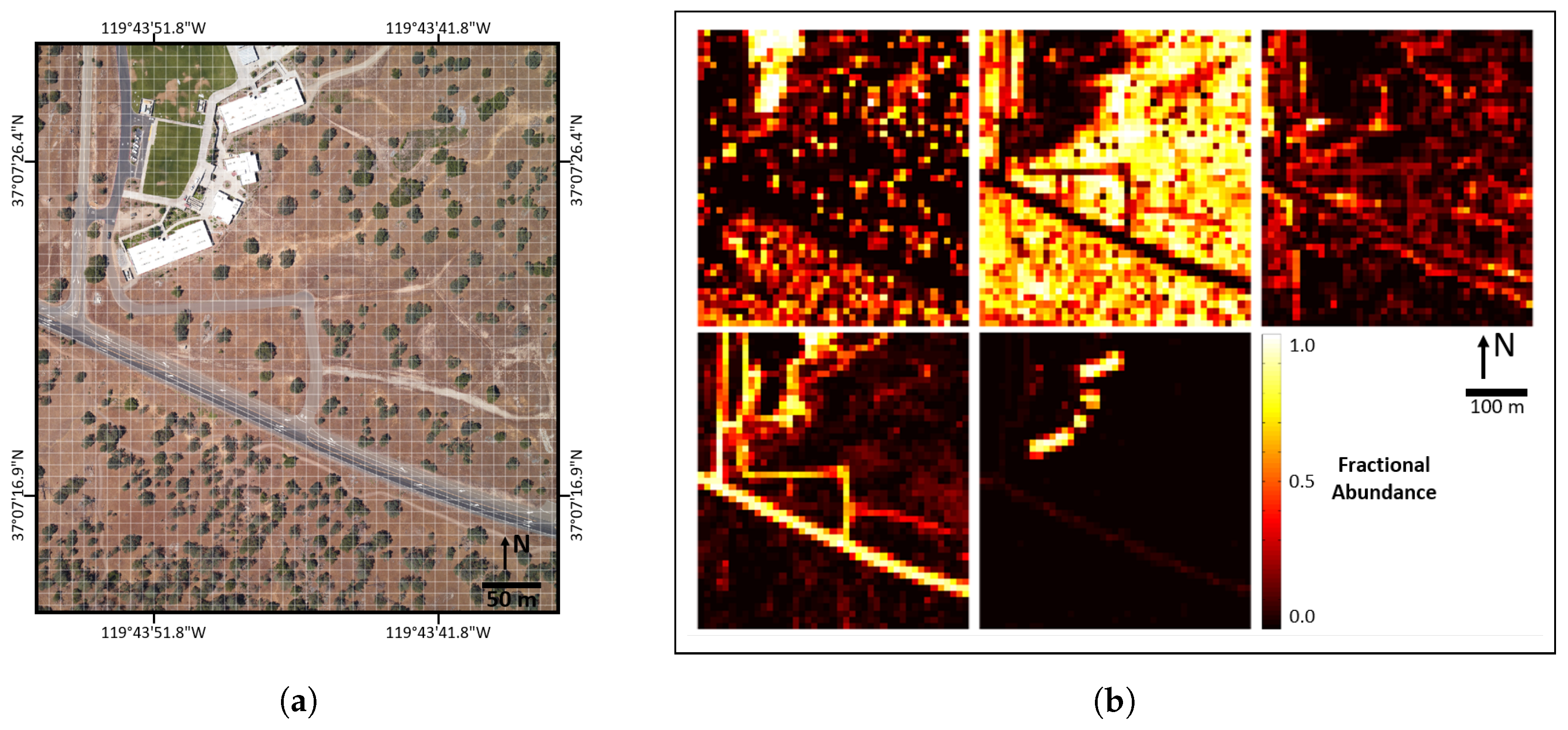
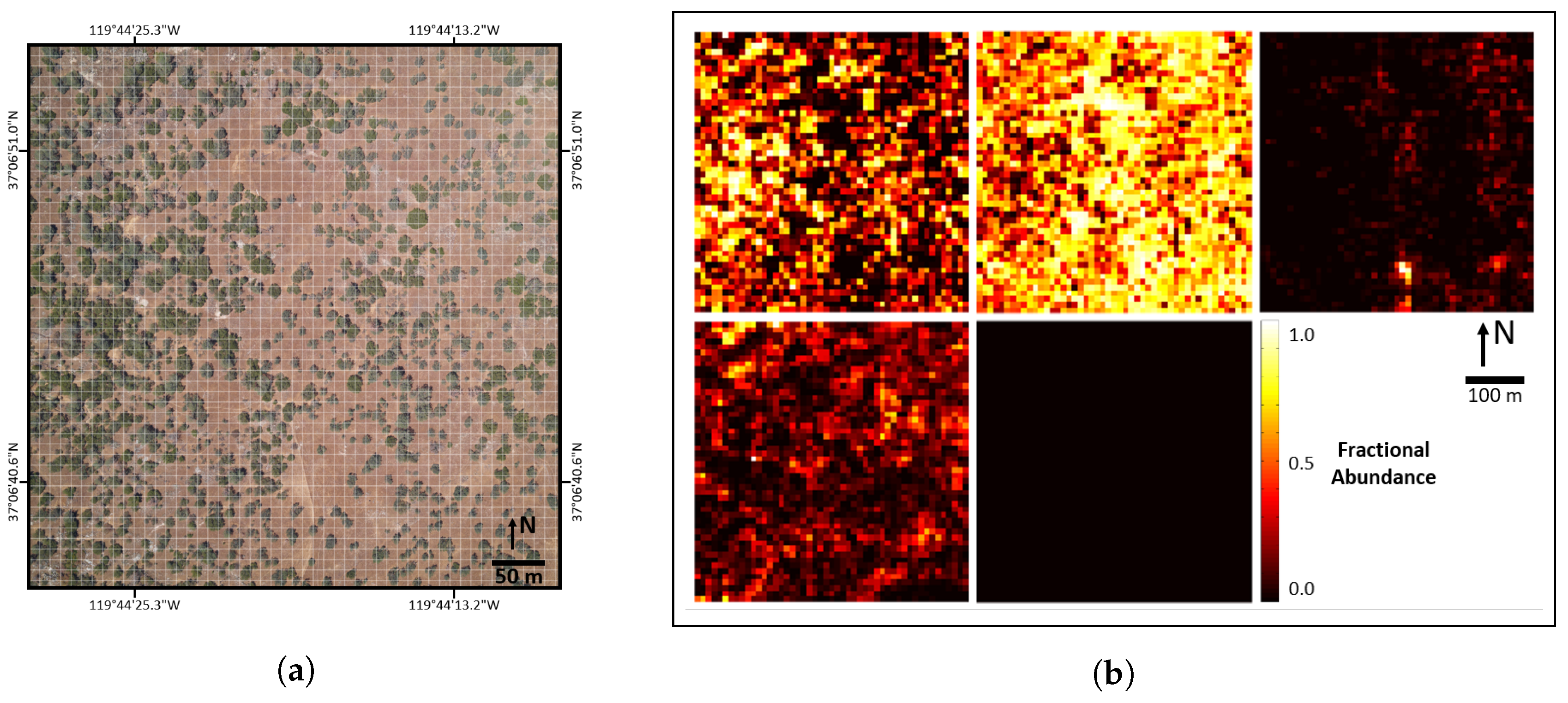
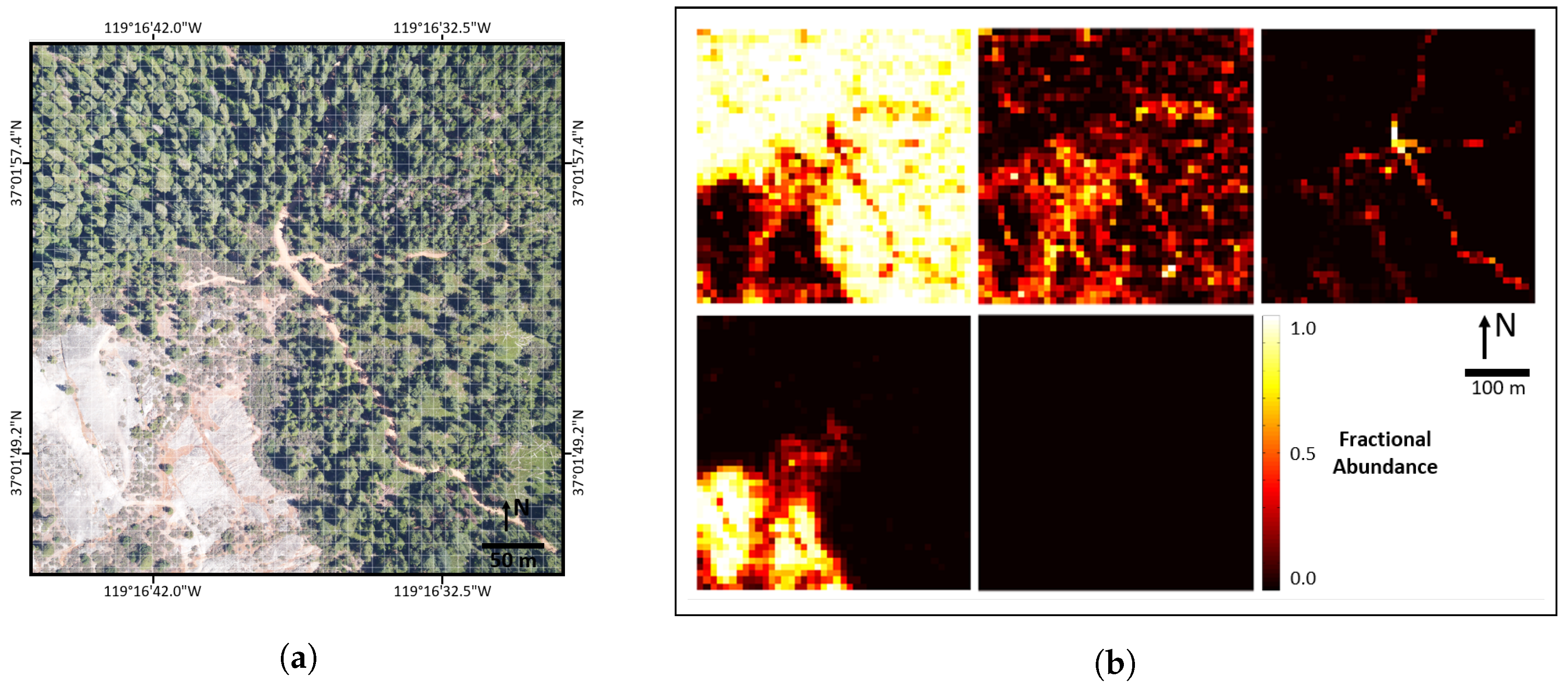
8], most of the pixels in a scene are composed of a mixture of classes. Spectral unmixing accounts for these mixed pixels and produces abundance maps, where each class has a corresponding abundance map that estimates the fraction of that class in each pixel. An example abundance map is shown in
Figure 1. Abundances for each pixel range from zero (0%) to one (100%), represented by black and white, respectively.
Reference data, or reference data maps, represent a specific type of map that is used to quantitatively assess how well a classification or spectral unmixing algorithm performs [
9]. Reference data maps are usually created through field surveys, imagery analysis, algorithms or a mixture of these methods [
10,
11,
12]. Reference data maps have often been called “ground truth” maps within the remote sensing community, but recently, there has been an effort to use reference data terminology [
9]. We strongly support this change, because the term ground truth is overused and implies that the maps are free of error.
Due to the large spatial extent of aerial imaging spectrometer scenes, generating new reference data maps is expensive and time consuming [
11,
13]. As a result, few reference data maps have been created, even though imaging spectrometers have been operational for several decades. Cuprite [
10], Indian Pines [
14], Salinas [
15] and Pavia [
12] are examples of commonly-used reference data products. Despite being widely used for several decades to assess the performance of new classification algorithms, we have not been able to locate validation reports that characterize the error or uncertainty in these reference data. Additionally, these products label whole pixels as belonging to classes, making them of little use for assessing the performance of spectral unmixing algorithms.
Researchers have used various methods to assess the performance of spectral unmixing algorithms. Qualitative assessments have visually compared unmixing results to well-known reference data, such as Cuprite, Indian Pines and Pavia [
7,
16,
17]. Quantitative assessments have used synthetic data [
7,
16,
17], average per-pixel residual error [
7,
18], taken the mean of several algorithms as the ideal and computed residuals from the ideal [
18], etc. Furthermore, there are several studies that have created sub-pixel reference data using high-resolution RGB videography [
19], RGB imagery [
20], multi-spectral imagery [
21] and IS imagery [
22]. However, although many of these studies alluded to the need for the validation of sub-pixel reference data, none implemented an assessment approach of reference data, nor did they expand on which reference data development approach is best suited to this challenge. This research therefore further explores the topic of sub-pixel reference data generated via high-resolution imagery.
In summary, the main challenges with reference data are that new reference data maps are prohibitively expensive to produce; existing reference data products have not been validated for accuracy; and we are not aware of any commonly-used reference datasets that contain abundance level detail.
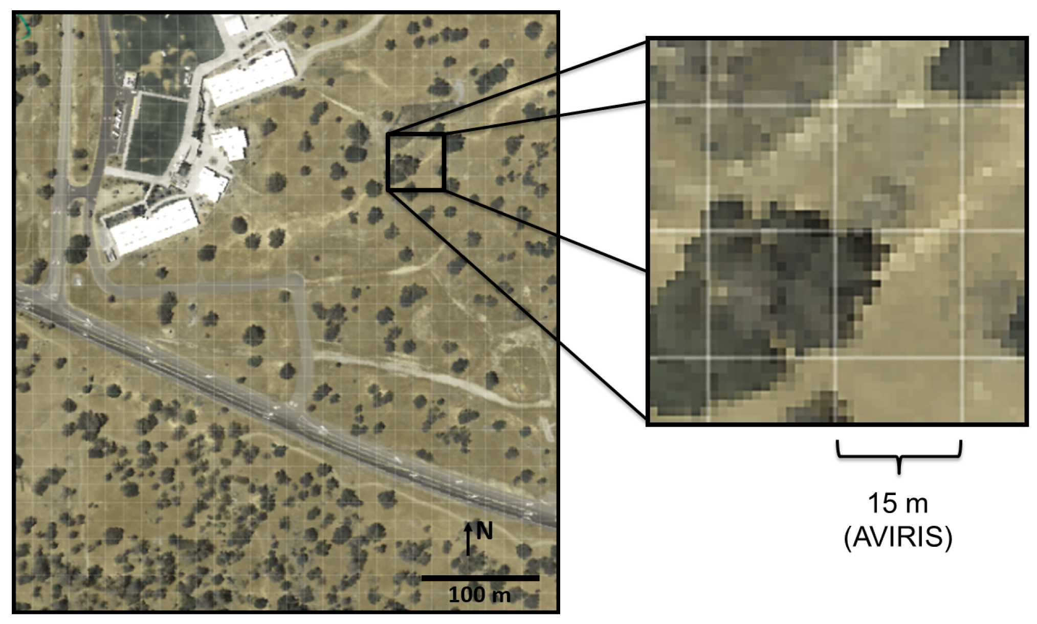
Our previous work [
23] proposed a new technique for efficiently generating abundance map reference data (AMRD). This technique is called remotely-sensed reference data (RSRD). RSRD aggregates the results of standard classification or spectral unmixing algorithms on fine-scale imaging spectrometer data (e.g., 1-m GSD National Ecological Observatory Network (NEON) IS data) to generate scene-wide AMRD for co-located coarse-scale imaging spectrometer data (e.g., 15-m GSD Airborne Visible-Infrared Imaging Spectrometer (AVIRIS) IS data), thereby enabling quantitative assessment of spectral unmixing algorithms. An example AVIRIS pixel grid pattern, overlaid on NEON imagery, is shown in
Figure 2.
The primary objective of this paper is to validate three AMRD scenes that were produced using the RSRD technique. The secondary objective of this paper is to promote the understanding that every method of generating reference data is vulnerable to certain types of error; reference data should not be used to assess classification or unmixing performance without a validation report that characterizes error and uncertainty in the reference data itself.
2. Methodology
2.1. Airborne Data and Cover Classes
The three scenes used throughout this paper are located on or adjacent to NEON D17 research sites near Fresno, CA [
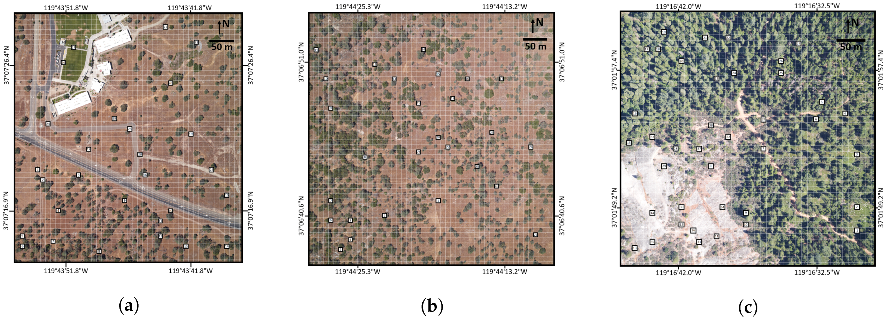
24]. Overhead images of the three scenes, collected by NEON’s co-mounted framing RGB camera, are shown in
Figure 3. Imagery over NEON D17 research sites was chosen for this study because NEON and AVIRIS conducted a joint campaign in June 2013, collecting imagery over the same areas on the same days [
25]. The three specific scenes were chosen to be representative of a wide variety of remote sensing scenes. The selected scenes include asphalt roads, dirt roads, concrete, buildings, grass fields, dry valley grasslands, high mountain forests, large rock outcroppings, etc. As such, the specific validation methods and conclusions in this paper should be generally applicable to many remote sensing scenes, especially environments dominated by rural or suburban features. It is worth noting that the intent of this research was to introduce the fine spatial resolution approach to coarser spatial resolution imaging spectroscopy pixel unmixing. Although we attempted to include both natural and man-made environments, we would not expect these scenes to be representative of dense urban environments.
During the June 2013 campaign, NEON collected 0.25-m GSD RGB and 1-m GSD IS data and AVIRIS collected 15-m GSD IS data. Imagery was provided to us in the orthorectified reflectance data format, including nearest neighbor resampling to a north-south-oriented grid. Further data details are listed in
Table 1. It is important to note that while we intend to produce AMRD specifically for AVIRIS data, the validation study in this paper was done for a generic 10-m GSD coarse-scale grid, allowing specific application for any imagery product with GSD larger than 10 m (i.e., AVIRIS, HyspIRI, Hyperion, EnMap, Landsat, etc.)
Through analysis of RGB imagery of the three scenes, we chose a classification scheme similar to common ecological studies [
26,
27]. The following is a list of the ground cover classes we chose for our three scenes:
Photosynthetic vegetation (PV): live green trees, bushes, weeds, grass, etc.
Non-photosynthetic vegetation (NPV): dead brown trees, bushes, weeds, grass, etc.
Bare soil (BS): undisturbed soil, sand, dirt trails, dirt roads, etc.
Rock: rocks, concrete, asphalt, etc.
Other: roof, metal, road paint, etc.
These classes represent the main ground constituents of our scenes, without over-complicating reference data generation and validation, i.e., they serve to illustrate the approach in this ecological context.
Historically, reference data maps have been generated using field surveys, imagery analysis, algorithms or a combination of multiple methods [
15]. Each of these methods for generating reference data has strengths and weaknesses. For example, field surveys provide the best situational awareness and ability to closely examine ground cover. However, they are subject to human error, such as bias, fatigue, mistakes, etc. Field surveys are also subject to perspective and positional error [
9]. Imagery analysis eliminates perspective and positional error, but reduces situational awareness and retains human error. Algorithms eliminate perspective and positional error, and reduce human error, but remove human intuition and situational awareness. Taking this information into account, the optimal method of generating reference data is not clear and will be further explored in this paper.
An important question for our study is how to validate and characterize the error in reference data, when reference data are already the most accurate estimates available. Our approach is to produce multiple independent versions of reference data for the same plots on the ground using traditional methods and RSRD and then to compare the results. To our knowledge, this is the first validated reference data presented at abundance-level spatial detail.
Time and budget constraints permitted the compilation of seven independent versions of reference data for 51 10 m×10 m plots, spread across the three scenes. Sample plots were selected using a pseudo-random number generator. The reference data methods and observers are listed below (
Supplementary S1):
Field surveys by Observer-A (Field-A)
Field surveys by Observer-B (Field-B)
Imagery analysis by Observer-A on NEON IS, aided by NEON RGB (Analyst-A)
Imagery analysis by Observer-B on NEON IS, aided by NEON RGB (Analyst-B)
RSRD by Euclidean distance (ED) on NEON IS (RSRD-ED)
RSRD by non-negative least squares (NNLS) spectral unmixing on NEON IS (RSRD-NNLS)
RSRD by maximum likelihood (ML) on NEON IS (RSRD-ML)
The observers were both graduate students in imaging science, i.e., a degree of familiarity with imaging products and image interpretation was assured.
Validation and characterization of error was accomplished by comparing each of these data to each other, as well as comparing each version of reference data to the mean of all (MOA) data. Through this analysis, we examined whether certain datasets were statistically different from one another, estimated the mean and standard deviation of differences from MOA and used equivalence hypothesis tests to determine statistical similarity to MOA.
2.2. Reference Data Collection
Validation of RSRD as a credible technique for producing AMRD is dependent on compiling multiple independent versions of reference data that are each of the highest quality. As such, our team compiled seven independent versions of reference data for 51 of the selected 10 m×10 m plots shown in
Figure 3. All but eight of the 51 plots were randomly selected, discarding plots that were located on busy roads, rooftops, etc. Eight non-randomly selected plots targeted under-represented cover types, such as asphalt, sidewalks and dirt roads. Due to time and budget constraints, private property issues, etc., the 51 plots were a subset of the original randomly selected plots.
The goal of reference data collection was to carefully estimate the abundance of ground cover classes in each of the 51 10 m×10 m plots, using field surveys, imagery analysis and RSRD methodologies. The following sections explain the details for each of these collection methodologies.
2.2.1. Field Surveys
Observers traveled to Fresno, CA, in summer 2016 and spent 12 days in the field measuring the abundance of ground cover classes in 51 10 m×10 m plots. The plots were spread nearly evenly across three scenes:
San Joaquin Experimental Range High School (SJERHS): the area surrounding Minarets High School, which lies adjacent to SJER on the north site of the range.
San Joaquin Experimental Range 116 (SJER116): the area surrounding NEON SJER field site #116.
Soaproot Saddle 299 (SOAP299): the area surrounding NEON SOAP field site #299.
Potential plots were chosen prior to the trip and are shown in
Figure 3. All of the potential plots were accessible, with the exception of SJERHS plots south of the main road, which are located on private, actively grazed, ranch land.
The landscape in SJERHS and SJER116 experienced little apparent change between 2013 imagery collection and 2016 field surveys; however, SOAP299 experienced a significant pine beetle infestation, resulting in the death of many trees in the area [
28]. This forced us to abandon most of the forest-dominated plots in SOAP299, instead focusing on plots with little apparent change, such as those dominated by dirt roads, bush, rock and soil.
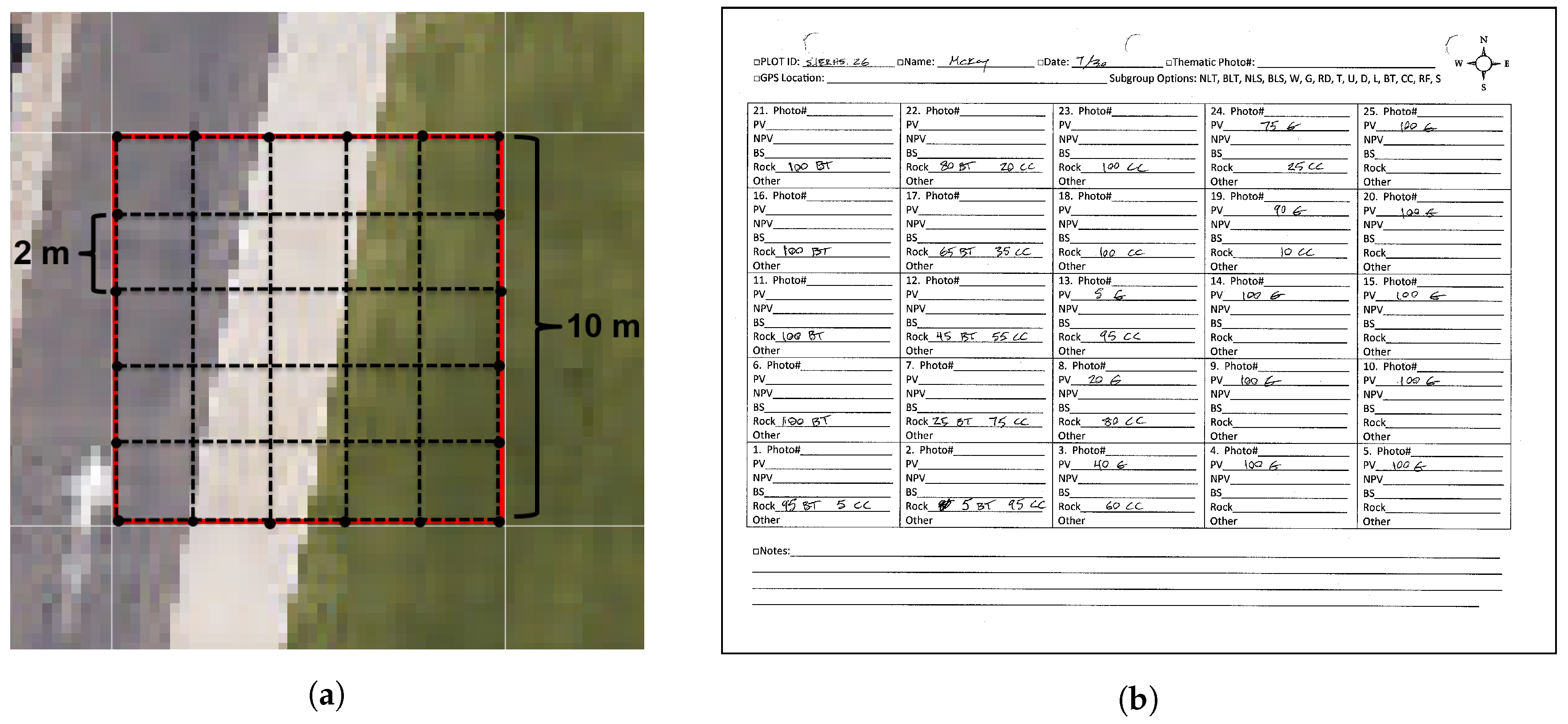
Approximate navigation to plot locations was accomplished using GPS-enabled smartphone mapping software and a compass. Fine placement of measurement grids was accomplished using detailed NEON RGB images of each plot, similar to
Figure 4a. In other words, our 10 m×10 m sampling grids were positioned by matching in-scene objects, rather than relying on the unknown precision of field GPS readings and imagery georeferencing; we assumed that this approach limited geospatial inaccuracies.
In order to more accurately estimate plot level abundances, a rope grid was positioned on top of the 10 m×10 m plot, dividing the plot into 25 2 m×2 m samples. This is illustrated in
Figure 4a. With the grid in place, the two observers independently estimated the abundance of ground cover classes in each of the 2 m×2 m samples. If the observers’ estimates differed by more than 15% cover area for a given class, the sample was re-examined by both researchers to reduce errors. Estimates were recorded on data collection sheets, as shown in
Figure 4b. In addition to abundance estimates for each 2 m×2 m sample, photos were captured showing the entire plot, near nadir photos were captured of each 2 m×2 m sample, GPS coordinates of plot center locations were measured, and a library of spectral samples was compiled using a Spectra Vista Corporation (SVC) field portable spectrometer. Paper data collection sheets and other data were compiled and recorded in a spreadsheet each evening so that errors and ambiguities could be resolved before forgetting important information.
2.2.2. Imagery Analysis
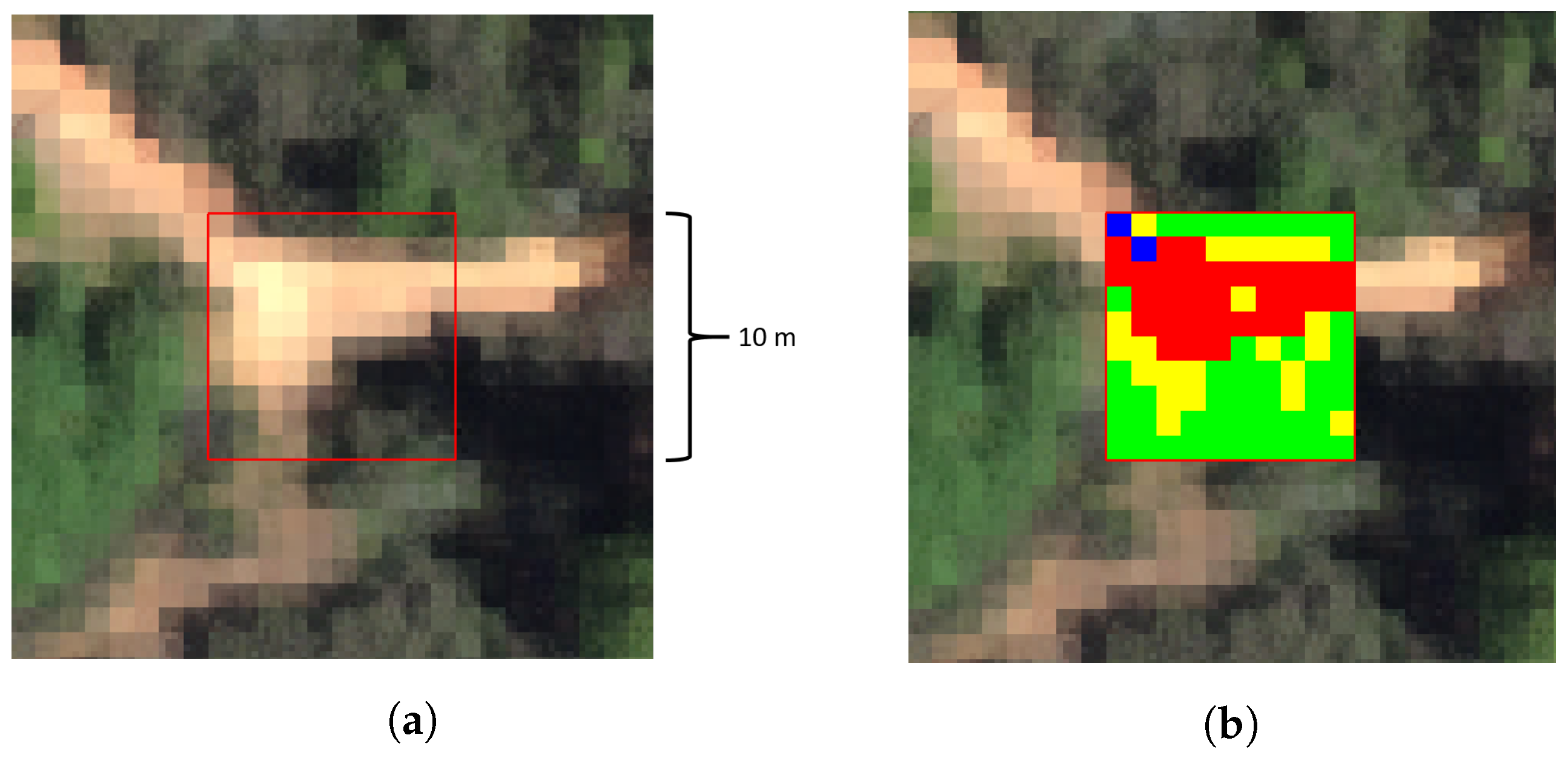
Imagery analyst-derived reference data were generated, corresponding to the same 51 plots estimated by the observers in the field. Instead of estimating fractional abundances for 25 2 m×2 m samples, as was done in the field, analyst reference data classified 100 1 m×1 m NEON IS whole pixels within each plot to one of the cover classes. Imagery analysis was performed several months after completing the field surveys, and field survey data were not consulted during imagery analysis. Analysis was accomplished in the ENVI 5.3 environment using pseudo-RGB visualizations of NEON IS data and NEON RGB imagery.
Figure 5 illustrates what the analysts saw as they classified the plots. This figure shows a hybrid view, where a pseudo-RGB view of NEON IS is 20% transparent on top of NEON RGB. The analyst was able to toggle between the hybrid view shown here, NEON IS and NEON RGB in order to make the best classification decision for the NEON IS pixels.
2.2.3. Remotely-Sensed Reference Data
Euclidean distance (ED) [
3], NNLS unmixing [
29] and ML [
3] were selected to estimate scene-wide AMRD using the RSRD technique. We chose these algorithms because of their widespread adoption, established reputation, and relative simplicity. This study was not intended to identify the best possible algorithm, i.e., we opted to use established methods to evaluate reference data outcomes.
Endmembers were extracted for each scene separately by selecting ten exemplar pixels for each cover class and taking their spectral mean. We opted for this approach, rather than algorithmic endmember extraction techniques, in order maintain human analyst control and interpretative intent over class representative spectra. The same endmembers were used for ED, NNLS and ML within each scene.
For ED, which is equivalent to a nearest-neighbor classifier, NEON IS pixels were evaluated using Equation (
1), where
x represents the spectrum of a pixel,
s is an endmember, and
n is the number of spectral bands. Pixels were assigned to the class whose endmember yielded the smallest distance. For NNLS, NEON IS pixels were represented by the linear mixture model in Equation (
2), where
a are abundances,
n is noise, and
M is the number of classes. Lawson’s implementation of non-negative least squares was used to solve for
a [
29]. It should be noted that while the NNLS algorithm does not impose a sum-to-one constraint, we later imposed this constraint on resulting abundances, such that ED, NNLS and ML methods all provided sum-to-one constrained solutions. For ML, initial prior probabilities,
, were obtained via spectral angle mapper (SAM) classification (Equation (
3)), then results were processed for ten iterations using Equation (
4), where
s represents the various ground cover classes. Final posterior probabilities were used as abundances. RSRD was performed on the entire SJERHS, SJER116 and SOAP299 scenes, with results corresponding to the 51 10 m×10 m plots extracted for comparison to field and analyst estimated reference data.
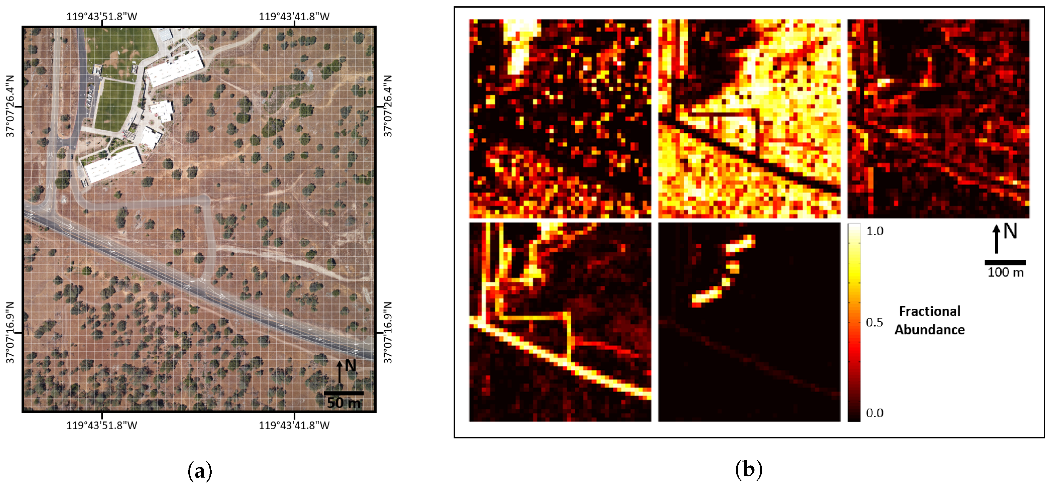
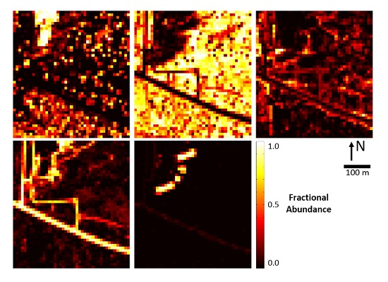
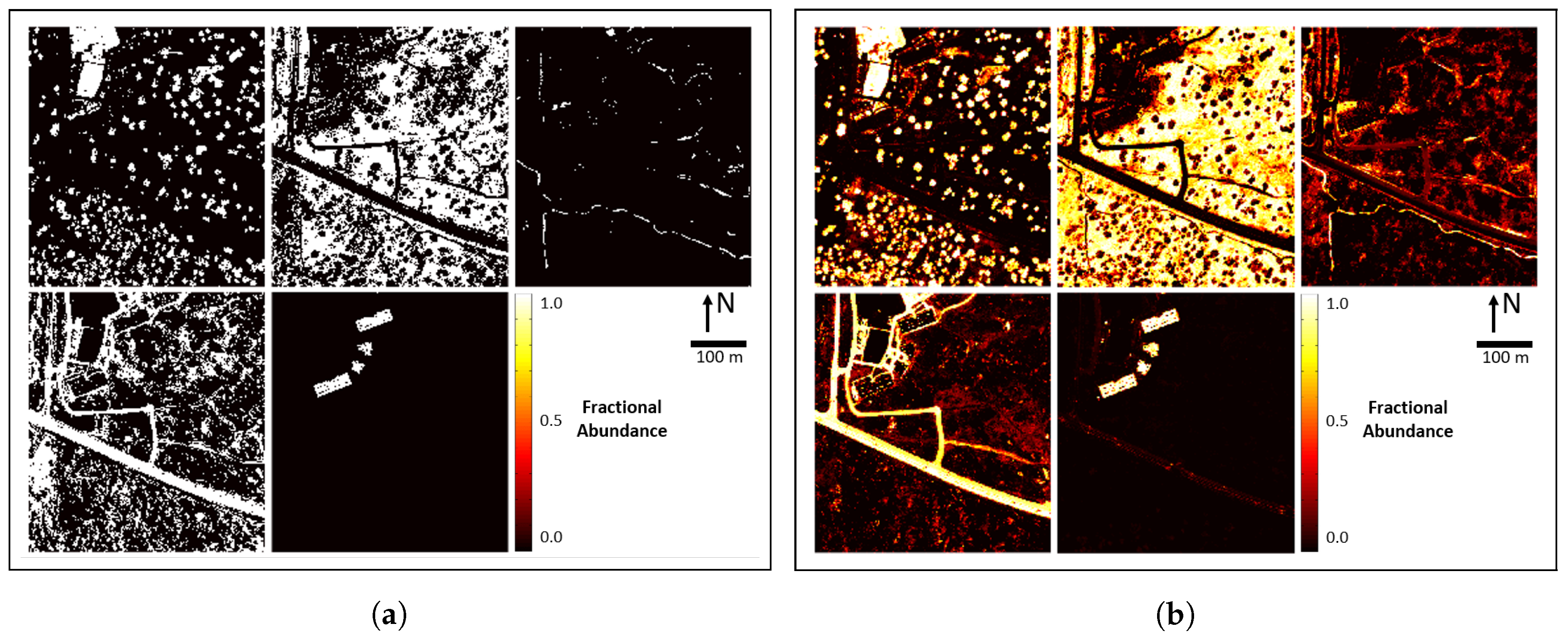
Figure 6 shows an example of fine-scale abundances generated using ED and NNLS. Both results are presented in abundance map format, even though ED assigns whole pixels to one class or another. For this reason, ED abundance maps are black and white, representing 0 (0%) or 1 (100%) coverage, while NNLS abundance maps have values ranging continuously from 0 to 1.
2.3. Data Aggregation
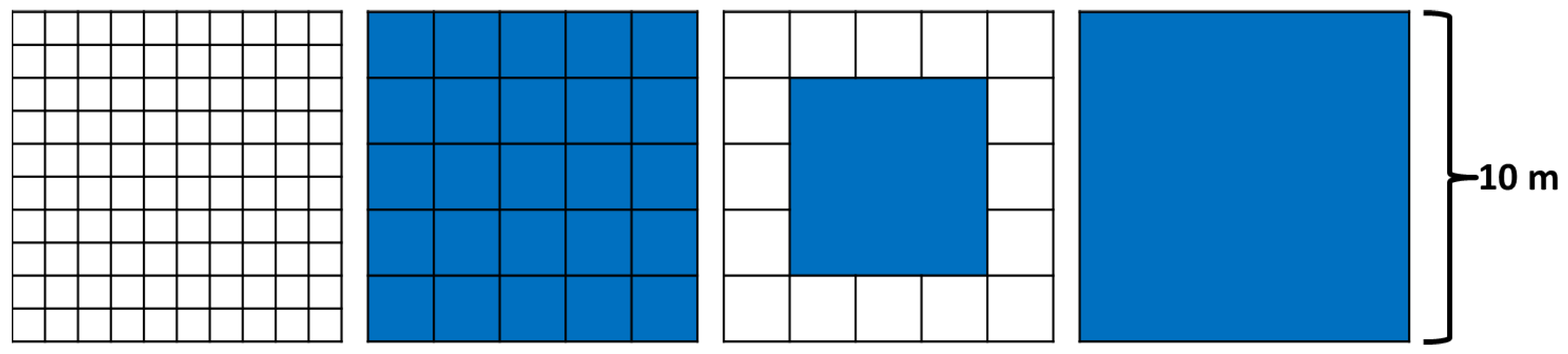
Field-A and Field-B data estimated abundances at the 2-m scale. Analyst-A, Analyst-B, RSRD-SAM and RSRD-ED classified whole NEON IS pixels at the 1-m scale. RSRD-NNLS and RSRD-ML estimated abundances at the 1-m scale. In order to directly compare field survey data with the other methods, 1-m scale data were aggregated to the 2-m scale through simple averaging of four 1-m samples. Further aggregation yielded 6 m and 10 m-scale data. Data aggregation is illustrated in
Figure 7. Note that aggregation at the 6-m scale excluded edge data.
Aggregating data and comparing results allowed us to build confidence that the RSRD methodology can be utilized to provide quality AMRD for any medium to large GSD imagery. As individual samples were aggregated to the 2-m, 6-m and 10-m scales, the variance of abundance estimates decreased, showing that the RSRD methodology, applied to 1-m NEON IS data, can be used to generate AMRD for any imagery with GSD greater than or equal to 10 m.
2.4. Methods of Data Comparison
Abundance map reference data estimates from the seven methods discussed above (Field-A, Field-B, Analyst-A, Analyst-B, RSRD-ED, RSRD-NNLS, RSRD-ML) were compared at the 2-m, 6-m and 10-m spatial aggregation scale. At the 2-m scale, there were 1275 data points for each of the seven versions of reference data, while 6-m and 10-m scale data each had 51 data points. Pairwise comparisons were made to evaluate how close each version was to the other versions. Each version was also compared to the mean of all (MOA) versions per plot and class. In making these comparisons, data were often subtracted from each other to produce difference data. Difference data were evaluated using histograms, statistical measures such as mean and standard deviation of differences, t-tests and equivalence tests.
When using a
t-test, the intention is to reject the null hypothesis, with the null hypothesis being that all data or treatments are the same. In other words,
t-tests are intended to demonstrate differences between datasets or treatments [
30]. The purpose of using
t-tests in this paper was to show that independent versions of reference data exhibit statistically significant differences from one another and, as such, need to be validated rather than simply assuming “ground truth”.
Failing to reject the null hypothesis does not prove similarity, but provides inconclusive results. Equivalence tests are similar to
t-tests, but are used to prove similarity. When using an equivalence test, the intention is still to reject the null hypothesis, but in this case, the null hypothesis is that data are different. Rejecting the null hypothesis in this case proves statistical equivalence. Equivalence tests require establishing a zone of equivalence,
. An equivalence test then finds the probability
p that
. If
, the data are proven equivalent with
% confidence [
31]. The purpose of using equivalence tests in this paper was to define equivalence zones wherein versions of reference data were statistically equivalent [
31] to MOA.
In practice, equivalence tests are performed by calculating confidence intervals for the difference between two datasets; if the entire confidence interval falls with the zone of equivalence, the two datasets are deemed statistically equivalent. It should also be noted that we want reference data to have both small mean and small standard deviation differences from one another; however, it is easier to “pass” statistical tests when data have a large standard deviation. For this reason, the mean and standard deviation of difference data are presented along with t-tests and equivalence tests.
3. Results
3.1. Comparison of Field Survey Data
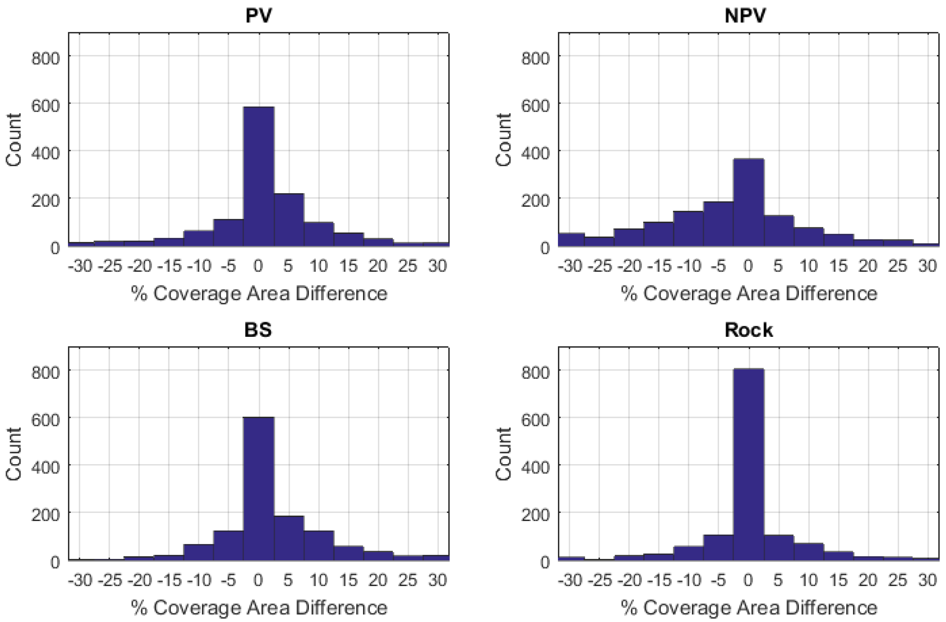
Histograms of the difference between Field-A and Field-B data at 2-m aggregation are presented in
Figure 8. These histograms highlight the frequency with which the observers differed by more than 15%, despite the careful collection procedures, which mandated re-assessment of any such samples. These histograms also demonstrate that difference data between the two field surveys were relatively Gaussian in shape, allowing for comparison using metrics such as the mean and standard deviation.
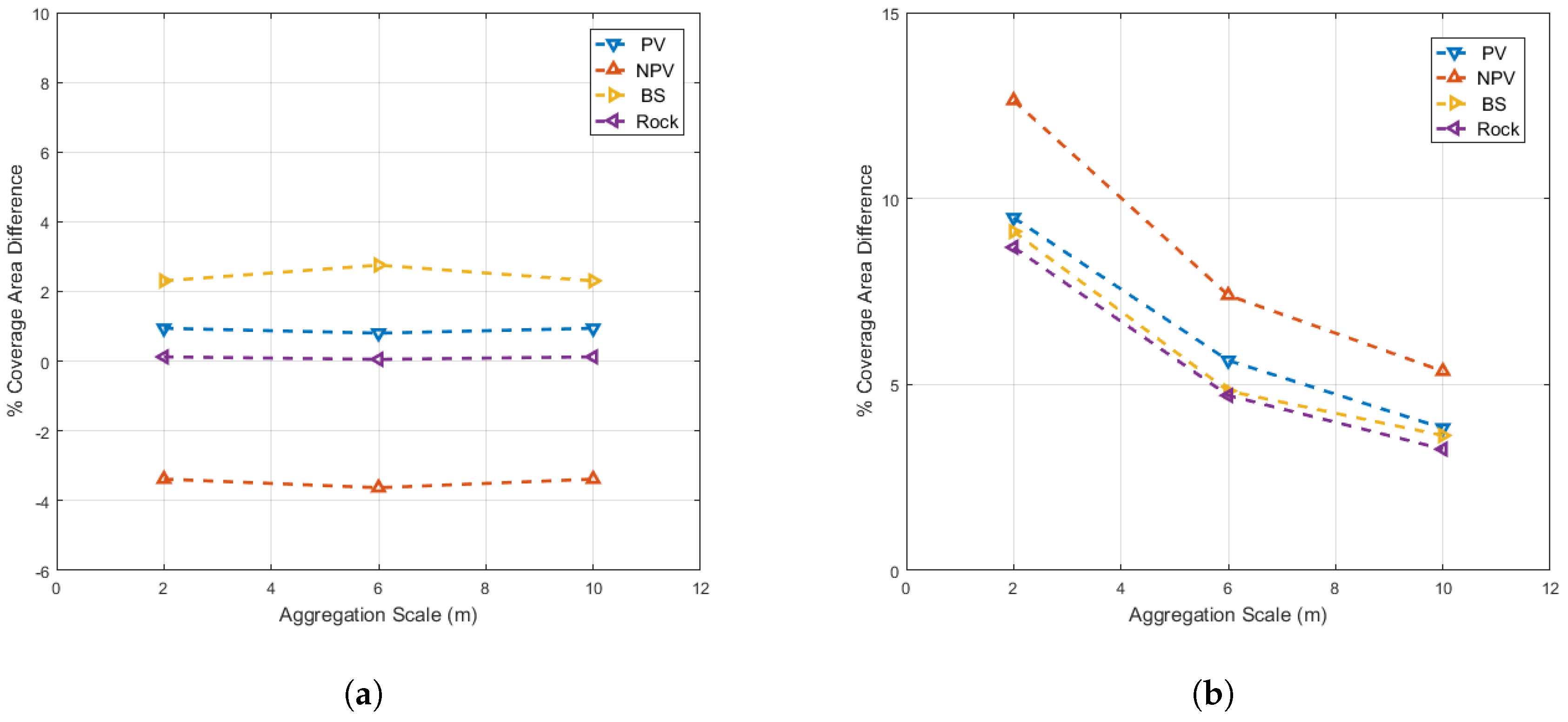
The mean and standard deviation of the data in
Figure 8 are presented in
Figure 9, along with the same data aggregated to 6 m and 10 m. Mean differences between samples at 2-m and 10-m aggregation ranged from
to 2.3%, depending on cover class. Mean differences only changed at the 6-m scale because edge samples were excluded in 6-m aggregation, as shown in
Figure 7. On average, Field-B data overestimated NPV and underestimated PV and BS when compared to Field-A data. Differences for rock were near zero mean.
As expected, aggregation to 6 m and 10 m data significantly reduced the variance of difference data. This reduction in variance occurred similarly for field survey, imagery analysis and RSRD-derived reference data, as they were aggregated from fine to coarse scale. The standard deviations of 2-m aggregation samples were 8.7 to 12.6%, depending on cover class, with NPV having the largest standard deviations. Not coincidentally, NPV is also the most abundant cover class in the scenes. When 2-m samples were aggregated to 6-m and 10-m plot sizes, the standard deviation decreased consistently. At 10-m aggregation, standard deviations dropped to 3.3 to 5.4%.
A
t-test rejects the null hypothesis when
.
, representing type I error, is typically set to 0.05 [
32]. In this case, the null hypothesis was that difference data had a zero mean.
Table 2 displays paired
t-test results for Field-A and Field-B data, along with the standard deviation of differences (
). The results indicate that statistically significant differences exist between the field observers’ estimates for all spatial levels of NPV and BS and PV at the 2-m scale.
3.2. Pairwise Comparisons of Reference Data Versions
In the previous section, Field-A and Field-B data were compared in some detail, including
Table 2, which showed
t-test results and standard deviations between the two datasets. In this section, we expand our pairwise comparisons to all seven versions of reference data and produce a similar table of
t-test results and standard deviations for pairwise comparisons at the 10-m aggregation scale.
Table 3 displays these results, with bold values indicating
, where the
t-test rejected the null hypothesis, indicating significant difference between data.
Each reference data version was compared to six other versions with four ground cover classes, resulting in 24 t-tests. The null hypothesis was rejected for at least half of the 24 t-tests for all reference data versions. Comparing field survey and imagery analysis methods only, the null hypothesis was rejected for 13 of the 24 t-tests. These results showed that our independent versions of reference data were significantly different from one another and that no single method stood out as the clear winner.
3.3. Comparison of Reference Data Versions to the Mean of All
Results from pairwise comparisons showed that various forms of carefully estimated reference data were significantly different. Furthermore, it was not clear which version of reference data was superior. Given these findings, we propose that for each plot and class, the mean of all (MOA) versions of reference data is more likely to represent true ground cover class abundances than any single method or observer. In this section, all reference data versions are compared to MOA, in order to determine which reference data approach was closest to the best available estimate of true abundances.
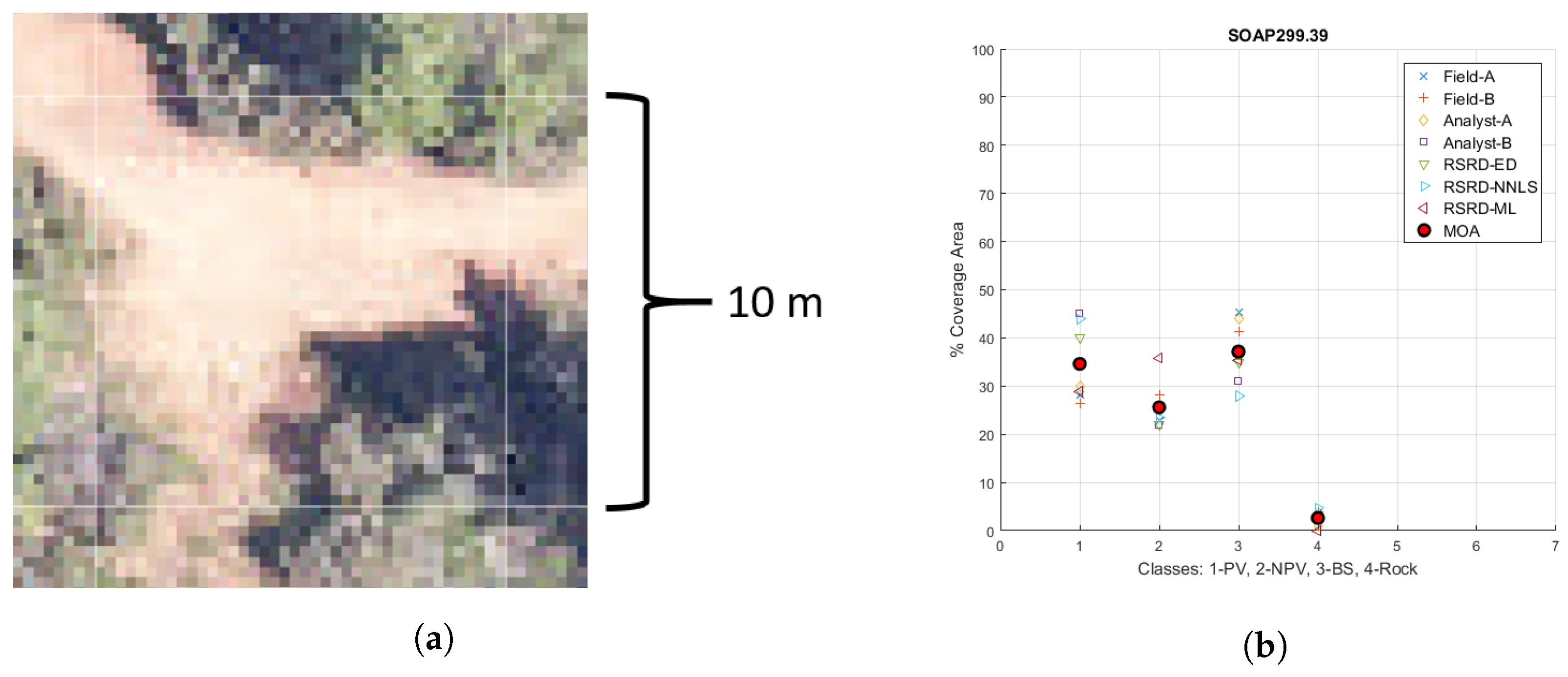
In order to better visualize the MOA concept, we present
Figure 10, which shows an example plot, along with abundance estimates from each version of reference data and MOA for each class. The variance among abundance estimates in
Figure 10 was near the median of our 51 sample plots. Difference from MOA data was calculated by subtracting MOA for each plot and class from the various reference data versions.
One way to explore which reference data method is closest to MOA would be to display difference data histograms, similar to
Figure 8, for each combination of different reference data methods and aggregation scales. However, we can also represent much of the information in a histogram by finding the center (mean) and spread (standard deviation) of difference data. To further streamline data presentation, we can combine mean and standard deviation data across classes. These data are presented in
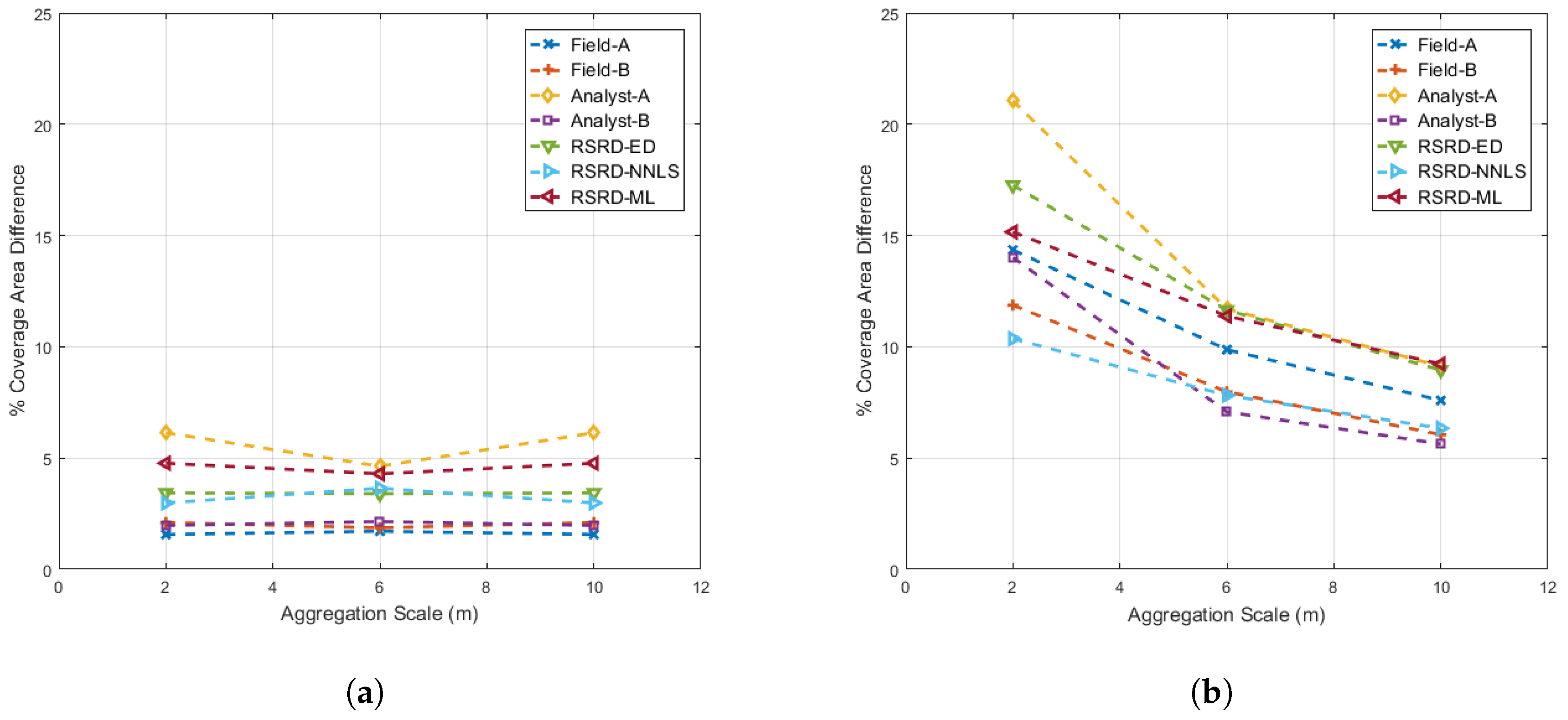
Figure 11.
Figure 11a displays the result of calculating the mean of difference data across 51 plots (histogram distribution center locations per class), then calculating the absolute value (otherwise, classes would cancel each other out) and then extracting the mean across classes.
Figure 11b displays the results of calculating the standard deviation of difference data across 51 plots (histogram distribution spread per class), followed by extracting the mean across classes.
Both plots in
Figure 11 are scaled from 0 to 25% coverage area to emphasize that mean differences from MOA (histogram distribution center locations) were relatively small compared to standard deviation differences. Examination of
Figure 11b suggests that Field-B, Analyst-B and RSRD-NNLS reference data estimates were more precise than Field-A, Analyst-A, RSRD-ED and RSRD-ML.
3.4. Statistical Equivalence Tests
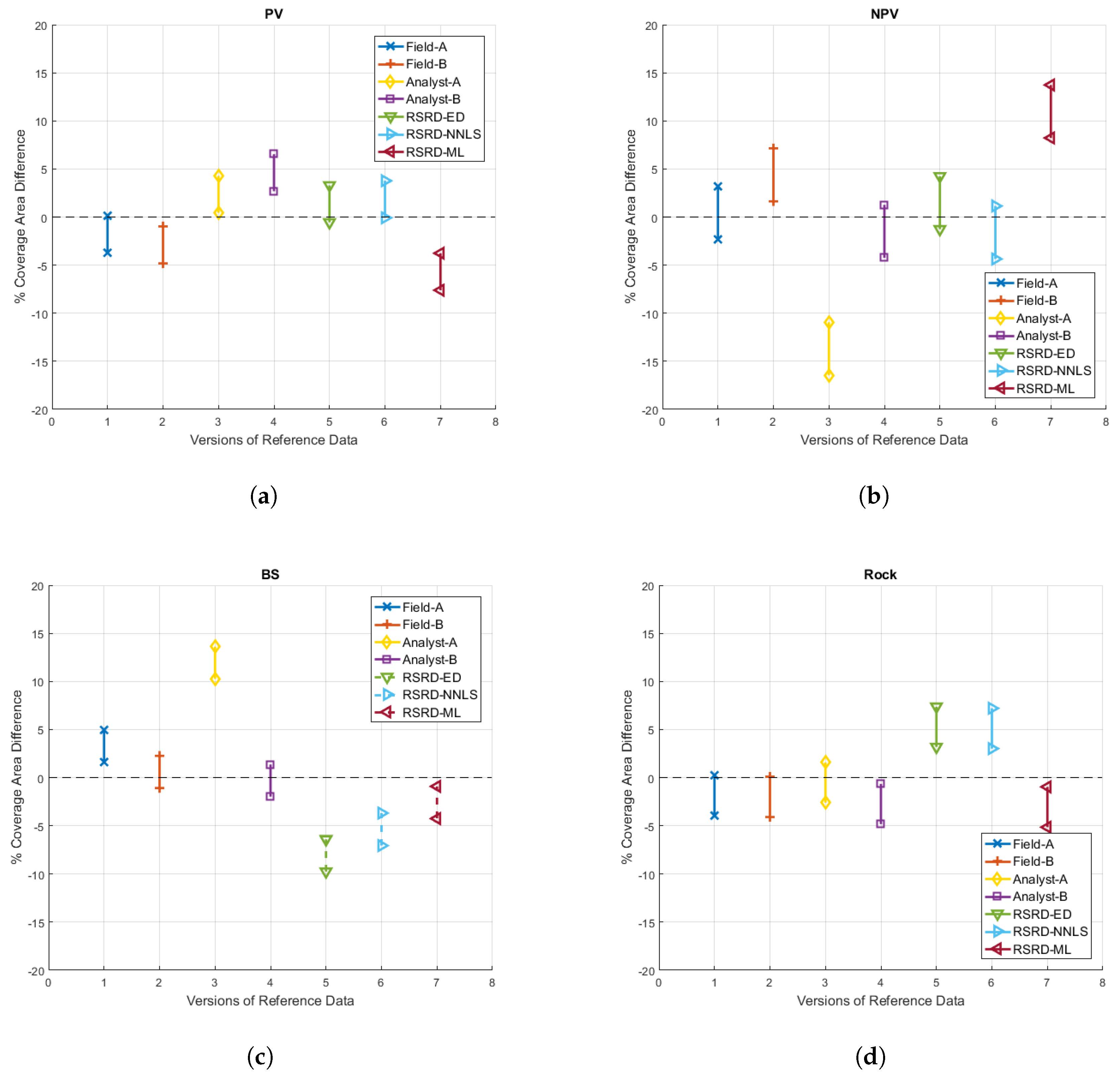
MATLAB R2016a’s ttest function provides confidence intervals that could be used for equivalence testing; however, we modeled all versions of our reference data within the Statistical Analysis Software (SAS OnDemand) general linear model (GLM) environment to produce more robust confidence intervals. The results of this analysis are provided in
Figure 12. It should be noted that for modeling purposes in the SAS GLM environment, we compared each reference data version to a linear combination of all other versions. This “leave-one-out” approach is slightly different than comparison to MOA, as MOA includes the data being compared. For this reason, SAS GLM confidence intervals are not perfectly centered on mean distance from MOA results displayed in subsequent tables.
The ideal confidence interval result would be narrow intervals centered on zero. Our results showed that the accuracy of reference data versions varied considerably across classes, e.g., Analyst-A data were the best version of reference data for rock, but were the worst version for NPV and BS. Among RSRD versions, RSRD-NNLS had the overall tightest zone of equivalence, with RSRD-ED a close second. Tabulated confidence interval data and the resulting equivalence zone are provided for RSRD-NNLS data in
Table 4. Note that the overall equivalence zone is simply the extent of extreme lower and upper CI values.
4. Discussion
As noted before, both field observers were graduate students in imaging science, with an emphasis in remote sensing, who carefully and independently estimated reference data for 1275 2 m×2 m samples, within 51 10 m×10 m plots. Their estimates were collected at the same time and compared in the field after every fifth sample to reduce the chances of human error. If any percent coverage estimate varied by 15% or more for any class, they each examined the 2 m×2 m sample again. Data were transferred to electronic form each evening with errors being corrected on the same day as data collection. Our field surveys were assumed to be of the highest quality that can reasonably be collected, and procedures were in place to reduce human error. Yet, despite this careful estimation of reference data, statistically significant differences existed between Field-A and Field-B data at 2-m, 6-m and 10-m spatial aggregation scales. Further examination revealed statistically significant differences between all our versions of reference data, and traditional methods of field surveys and imagery analysis faired no better than RSRD methods.
It should be noted that the standard deviation of differences between Field-A and Field-B data were smaller than for the other pairwise comparisons. This may indicate that field surveys were the most dependable way to produce accurate reference data. However, it should also be noted that the field survey data may have been less independent than the other versions. The observers worked in tandem throughout the field surveys. While they each independently estimated all 1275 2 m×2 m samples, the collection procedures included comparing results every five samples in an effort to reduce errors and mistakes. This process of checking answers inevitably had some effect on abundance estimation decisions.
The t-test results in this paper are a reminder that even carefully generated reference data are not perfectly accurate and should be validated prior to use in assessing other algorithms. In the past, remote sensing algorithm papers generally have not discussed the accuracy of reference data and often have not cited how reference data were created. Given the results in this paper, we encourage a more robust treatment of reference data in the remote sensing community.
Having used t-tests to demonstrate significant differences between versions of reference data, in order to reinforce the importance of accuracy validation, we now turn our attention toward determining the degree of similarity among reference data. We accomplished this by examining the mean and standard deviation of differences, as well as confidence intervals and resulting zones of equivalence.
We interpreted mean differences as absolute bias between different forms of reference data, i.e., Observer-A “saw” less NPV on average than Observer-B. These biases between reference data versions and MOA were relatively similar across reference data versions. Standard deviation of differences from MOA, on the other hand, were interpreted as the steadiness or reliability of each reference data estimate, i.e., Observer-B’s estimates were reliably close to MOA and there were few outliers. These mean and standard deviation differences can be equated to accuracy and precision, respectively. Spatial aggregation of reference data from 2 m to 10 m did not decrease mean differences; however, aggregation significantly and predictably reduced standard deviation differences.
This reduction in variance with spatial aggregation was a positive trend, showing the power of the RSRD concept of aggregating many fine-scale pixels to produce AMRD for coarse-scale imagery. We expect that aggregation to coarse imagery with GSD >10 m would result in little change to mean differences, but would further reduce standard deviation differences. As such, we consider the validation in this paper to be valid for any coarse imagery with GSD >10 m.
Statistical analysis of difference data revealed that Field-B, Analyst-B and RSRD-NNLS versions of reference data were the closest versions to MOA. Analyst-B appeared to represent the best overall version of reference data when compared to MOA, with a mean difference of 2.0% and a standard deviation of 5.6% at 10-m aggregation. RSRD-NNLS was nearly as accurate and precise, with a mean difference of 3.0% and standard deviation of 6.3%. Furthermore, RSRD-NNLS also had the tightest overall zone of equivalence among RSRD versions, .
It should be noted here that the generation of MOA required significant effort for just 51 plots of data and would be unrealistic across large spatial extents. Similarly, the generation of scene-wide AMRD using traditional field survey or imagery analysis methods would be unsustainable. As such, the MOA concept is used to validate the accuracy of scene-wide AMRD generated using the RSRD technique. Based on standard deviation differences and zones of equivalence, we selected RSRD-NNLS to serve as validated scene-wide AMRD.
We considered using the best case version of RSRD for each ground cover class in an effort to reduce the expected error and uncertainty in the final reference data. However, constructing scene-wide AMRD from different algorithms would introduce sum-to-one error (an assumption in many unmixing algorithms) in the final abundances, and correcting this would introduce another source of error.
Using the NNLS implementation of RSRD to produce scene-wide AMRD for our three scenes yields
Figure 13,
Figure 14 and
Figure 15. The accuracy of these reference data has been validated in this paper, resulting in the data provided in
Table 5.
5. Conclusions
The purpose of this paper was to validate abundance map reference data (AMRD) generated using the remotely-sensed reference data (RSRD) technique, which aggregates classification or unmixing results from fine-scale imaging spectrometer (IS) data to produce AMRD for co-located coarse-scale IS data. This validation effort included three separate remote sensing scenes. The scenes were specifically chosen to be representative of many remote sensing environments. They contain a variety of common ground cover, including asphalt roads, dirt roads, concrete, buildings, grass fields, dry valley grasslands, high mountain forests, large rock outcroppings, etc. Therefore, we expect the conclusions of this paper to be generally applicable to similar rural and suburban scenes. We recommend that additional validation studies focus on more diverse and even densely-mixed land cover types.
Validation was accomplished by estimating AMRD in 51 randomly selected 10 m×10 m plots, using seven different methods or observers, and comparing the results. These independent versions of reference data included field surveys by two observers, imagery analysis by two observers and RSRD by three algorithms. Given that t-test comparisons showed statistically significant differences between all seven versions of reference data, we proposed that the best estimate of actual ground cover abundance fractions within the 51 plots is found by taking the mean of all (MOA) independent versions of reference data for each plot and class. Generating MOA for a limited number of random plots is labor intensive, but once generated, MOA can then be used to validate AMRD generated using the RSRD technique, which efficiently produces scene-wide reference data and can serve as a validated baseline for all future algorithm developments.
At the 10-m GSD aggregation scale, mean differences between versions of reference data and MOA were 1.6 to 6.1%, with standard deviations of 5.6 to 9.2%. The closest version of reference data to MOA was a version of imagery analysis, with mean differences of 2.0% and a standard deviation of 5.6%. The RSRD algorithm based on NNLS spectral unmixing was nearly as close to MOA, achieving mean differences of 3.0% and a standard deviation of 6.3%. Equivalence testing yielded a zone of equivalence between for RSRD-NNLS. Considering the efficiency of RSRD in producing scene-wide AMRD, these results are promising. Validated scene-wide AMRD generated using RSRD-NNLS are available for use by the remote sensing community.
The novel contributions to the pixel unmixing branch of remote sensing research include: (1) a documented validation of the accuracy of abundance map reference data (AMRD) itself; (2) the inclusion of five reference data classes, which is similar to many contemporary classification/unmixing efforts; and (3) the creation and validation of AMRD for three new study scenes using different IS sensors. Secondary goals are to make the larger remote sensing community more aware of the need to validate reference data itself and to establish methods to quantitatively assess the performance of spectral unmixing algorithms.
This validation effort centered around using generic 10-m GSD coarse-scale imagery, which was designed such that the reference data accuracy validation in this paper would be valid for use with any coarse imagery with GSD >10 m. The next step of our research is to apply the validated AMRD to examples of real coarse-scale imagery, such as the AVIRIS data mentioned previously. Applying AMRD to real imagery requires addressing various important topics, including the sub-pixel spatial alignment of fine- and coarse-scale imagery (critical to overlaying imagery with different spatial resolutions), comparing aggregation strategies, such as simple rectangular pixel aggregation and sensor point-spread function (PSF) aggregation, and the introduction of methods to compare coarse unmixing results to AMRD.


 and
and 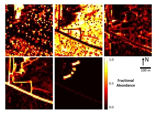


