SMOS-IC: An Alternative SMOS Soil Moisture and Vegetation Optical Depth Product

Abstract

The main goal of the Soil Moisture and Ocean Salinity (SMOS) mission over land surfaces is the production of global maps of soil moisture (SM) and vegetation optical depth (τ) based on multi-angular brightness temperature (TB) measurements at L-band. The operational SMOS Level 2 and Level 3 soil moisture algorithms account for different surface effects, such as vegetation opacity and soil roughness at 4 km resolution, in order to produce global retrievals of SM and τ. In this study, we present an alternative SMOS product that was developed by INRA (Institut National de la Recherche Agronomique) and CESBIO (Centre d’Etudes Spatiales de la BIOsphère). One of the main goals of this SMOS-INRA-CESBIO (SMOS-IC) product is to be as independent as possible from auxiliary data. The SMOS-IC product provides daily SM and τ at the global scale and differs from the operational SMOS Level 3 (SMOSL3) product in the treatment of retrievals over heterogeneous pixels. Specifically, SMOS-IC is much simpler and does not account for corrections associated with the antenna pattern and the complex SMOS viewing angle geometry. It considers pixels as homogeneous to avoid uncertainties and errors linked to inconsistent auxiliary datasets which are used to characterize the pixel heterogeneity in the SMOS L3 algorithm. SMOS-IC also differs from the current SMOSL3 product (Version 300, V300) in the values of the effective vegetation scattering albedo (ω) and soil roughness parameters. An inter-comparison is presented in this study based on the use of ECMWF (European Center for Medium range Weather Forecasting) SM outputs and NDVI (Normalized Difference Vegetation Index) from MODIS (Moderate-Resolution Imaging Spectroradiometer). A six-year (2010–2015) inter-comparison of the SMOS products SMOS-IC and SMOSL3 SM (V300) with ECMWF SM yielded higher correlations and lower ubRMSD (unbiased root mean square difference) for SMOS-IC over most of the pixels. In terms of τ, SMOS-IC τ was found to be better correlated to MODIS NDVI in most regions of the globe, with the exception of the Amazonian basin and the northern mid-latitudes.

1. Introduction

The estimation of surface soil moisture (SM) at global scale is a key objective for the recent L-band microwave missions SMOS (Soil Moisture and Ocean Salinity) (Kerr et al., 2012 [1]) and SMAP (Soil Moisture Active Passive) (Entekhabi et al., 2010 [2]). Measurements of soil moisture are needed for applications related to the study of climate change or agriculture (droughts, floods, etc.) and hydrological processes (Brocca et al., 2010 [3]) such as precipitation, infiltration, runoff and evaporation. Moreover, SM is considered as an Essential Climate Variable (ECV) and it is included in in the Climate Change Initiative (CCI) project (Hollmann et al., 2013 [4]). An ECV is defined as a physical, chemical or biological variable that critically contributes to the characterization of the Earth’s climate.

The soil moisture of the first 2–3 cm soil layer is highly related to the soil emissivity at L-band through the soil permittivity. SMOS uses an interferometric radiometer, which delivers multi-angular brightness temperature measurements at L-band. Currently, various products are derived from the SMOS data at Level 2 (Kerr et al., 2012 [1]) and at Level 3 (Al Bitar et al., 2017 [5]), such as the SMOSL3 Brightness Temperature (SMOSL3 TB) and the SMOSL3 SM and τ products, with a 625 km² sampling. The SMOS SM retrieval algorithm, which is common to both SMOS Level 2 (L2) and Level 3 (L3) products, has been continuously improved since the launch of the satellite in 2009 (Kerr et al., 2001 [6]; Mialon et al., 2015 [7]; Al Bitar et al., 2017 [5]). It has been evaluated against several datasets from various space-borne sensors such as SMAP, the active Advanced Scatterometer (ASCAT), the Advanced Microwave Scanning Radiometer (AMSR-E) or different versions of the SMOS products (Al-Yaari et al., 2014 [8]; Al-Yaari et al., 2015 [9], 2017 [10], Kerr et al., 2016 [11]). All versions of the Level 2 (L2) and Level 3 (L3) products, are based on the inversion of the L-band Microwave Emission of the Biosphere (L-MEB) radiative transfer model (Wigneron et al., 2017 [12], thus retrieving two main parameters: soil moisture and vegetation optical depth at nadir (τ).

The SMOS τ is a measure of the attenuation of the microwave radiations by the vegetation canopy at L-band. Vegetation is commonly studied at optical or infrared frequencies. However, the longer wavelength of L-band sensors allows penetration of the radiations within the canopy. Thus, τ can be related to different vegetation features such as forest height (Rahmoune et al., 2013 [13], 2014 [14]), vegetation structure (Schwank et al., 2005 [15], 2012 [16]), water content (Jackson and Schmugge, 1991 [17], Mo et al., 1982 [18], Wigneron et al., 1995 [19]; Grant et al., 2012 [20]), sapflow (Schneebeli et al., 2011 [21]) and leaf fall (Guglielmetti et al., 2008 [22]; Patton et al., 2012 [23]). Furthermore, some vegetation indices can also be related to τ such as the Leaf Area Index (LAI) (Wigneron et al., 2007 [24]) and the normalized difference vegetation index (NDVI) (Grant et al., 2016 [25]). Note that some studies have also demonstrated the notable influence of soil roughness on the retrieved values of the τ parameter at both local and regional scales (Patton et al., 2013 [23]; Fernandez-Moran et al., 2015 [26]; Parrens et al., 2017 [27]).

The L-MEB model has been progressively refined and improved (Wigneron et al., 2011 [28], 2017 [12]). The SMOS L2 and L3 algorithms are based on a bottom-up approach where the TB contributions of 4 x 4 km land cover surfaces are convoluted using the antenna pattern to upscale the TB simulations to the sensor resolution. The use of such a bottom-up approach to retrieve SM and τ presents two main drawbacks. First, this approach is impacted by the uncertainties associated with the higher resolution auxiliary files, like the land cover maps, which are used to characterize the pixel heterogeneity. Second, the approach is more time consuming as the exact antenna patterns have to be applied for each view angle.

In this study, an alternative SMOS product is presented, hereinafter referred to as SMOS-IC (SMOS-INRA-CESBIO). This product is based on a simplified approach developed by INRA (Institut National de la Recherche Agronomique) and CESBIO (Centre d’Etudes Spatiales de la BIOsphère) and differs from the operational SMOS Level 2 and Level 3 products in four main ways:

I

The main objective of this product is to be as independent as possible from auxiliary data. The SMOS-IC algorithm does not take into consideration pixel land use and assumes the pixel to be homogeneous as suggested by Wigneron et al., 2012 [29]. The SM and τ retrieval is performed over the whole pixel rather than over the fraction designated as either low vegetation or forest. Note that this approach is similar to the one considered in the development of the AMSR-E and SMAP SM algorithms (O’Neill et al., 2012 [27]). By simplifying the retrieval approach, the SMOS-IC product becomes independent of the ECMWF soil moisture information currently used as auxiliary information to estimate TB in the subordinate pixel fractions of heterogeneous pixels in the operational SMOS L2 and L3 algorithms (Kerr et al., 2012 [1]).

II

In relation to the above point, in some cases, the Level 2 and Level 3 algorithms use values of LAI derived from MODIS [30] to initialize the value of optical depth in the inversion algorithm (Kerr et al., 2012 [1]). In SMOS-IC, this is not implemented, and the initialization of optical depth in the inversion algorithm is based on a very simple approach (given in the following) and is completely independent of the MODIS data.

III

SMOS-IC uses as input SMOS Level 3 fixed angle bins Brightness Temperature (TB) data at the top of the atmosphere and contains different flags allowing to filter SM retrievals accounting for the quality of the input TB data and for the TB angular range in the L-MEB inversion. SMOS-IC does not make use of the computationally expensive corrections based on angular antenna patterns to account for pixel heterogeneity as in the L2 and L3 retrieval algorithms.

IV

New values of the effective vegetation scattering albedo (ω) and soil roughness parameters (H_R, N_RV, and N_RH) are considered in the SMOS-IC product. This change is based on the results of Fernandez-Moran et al. (2016) [31] who calibrated the L-MEB vegetation and soil parameters for different land cover types based on the International Geosphere-Biosphere Programme (IGBP) classes, as well as the findings of Parrens et al. (2016) [32] who computed a global map of the soil roughness H_R values. The calibration of Fernandez-Moran et al. (2016) [31] was obtained by selecting the values of the parameters (H_R, N_RV, N_RH, and ω) which optimized the SMOS SM retrievals, with respect to the in situ SM values measured over numerous sites obtained from ISMN (International Soil Moisture Network). The parameter values resulting from this new calibration differ from those used in the current SMOS L2 and L3 products. Values currently used in the SMOS L2 and L3 algorithms (Kerr et al., 2012 [1]) were defined before launch from literature. Over forested areas, values were updated but not over low vegetation. Consequently, in Version 620 of the L2 (and Version 300 for L3) algorithm, ω is still assumed to be zero over low vegetation canopies and ω ~ 0.06–0.08 over forests. Similarly, H_R is equal to 0.3 for forests and H_R = 0.1 for the rest of the cover types, whereas N_RH and N_RV are respectively set to 2 and 0 at global scale.

An evaluation and calibration of SMOS-IC at local scale was performed in Fernandez-Moran et al. (2016) [31]. The present study aims at presenting SMOS-IC and illustrating the main features of the SMOS-IC SM and τ products at global scale, in comparison to the current SMOSL3 product. To achieve this, the SMOS-IC and SMOSL3 SM products were compared against the ECMWF SM product for ease of comparison. Furthermore, NDVI (Rouse et al., 1974 [33]) from the Moderate-Resolution Imaging Spectroradiometer (MODIS) was used as a vegetation index to analyze the seasonal changes in the τ products from both SMOS-IC and SMOSL3. The NDVI index which is derived from optical observations cannot be directly compared to the τ product, which is derived from microwave observations. It must be noted that the L-band TB observations are almost insensitive to green leaves (Guglielmetti et al., 2007 [34], Santi et al., 2009 [35]), and τ is related to the vegetation water content (VWC, kg/m²) of the whole vegetation layer. However, the NDVI index is a good indicator of the vegetation density and it can be used to interpret the seasonal changes in the SMOS τ product at large scale over low vegetation as found by Grant et al. (2016) [25], but with some caveats: saturation effects at high levels of vegetation density, sensitivity to the effects of snow and soil reflectivity (Qi et al., 1994 [36]), etc. It may be noted that NDVI is the proxy used for estimating τ in the current operational algorithm of the SMAP mission (O’Neill et al., 2012 [37]).

In Section 2, we present a description of both SMOS algorithms (SMOSL3 and SMOS-IC) and of the MODIS NDVI and ECMWF SM datasets. The inter-comparison of the SMOS products in terms of soil moisture and vegetation optical depth is given in Section 3. The inter-comparison covers almost six years of data, from 2010 to 2015, excluding the commissioning phase (the first six months of 2010; Corbella et al., 2011 [38]). Discussion and conclusions are presented in Section 4.

2. Materials and Methods

2.1. SMOSL3 Brightness Temperature, Soil Moisture and Vegetation Optical Depth

At Level 3, there are different SMOS products (Al Bitar et al., 2017 [5]). In this study, we used the SMOS L3 products which include TB, τ and SM (version 300) data produced by the CATDS (Centre Aval de Traitement des Données SMOS) (Al Bitar et al., 2017 [5]). These products are available in the NetCDF format and on the Equal-Area Scalable Earth (EASE) 2.0 grid (Armstrong et. al, 1997 [39]) with a 625 km² sampling [40]. The SMOSL3 TB is measured at the top of the atmosphere and provided in the surface reference frame (i.e., H and V polarizations) at angles ranging from 2.5 ± 2.5 to 62.5 ± 2.5. Ascending (~06:00 LST at the equator) and descending (~18:00 LST) orbits are processed separately. The Level 3 processor uses the same physically based forward model (L-MEB) as the ESA SMOS Level 2 processor (Kerr et al., 2012 [1], Kerr et al., 2013 [41]) for the retrieval of both SM and τ from dual polarization (H, V) and multi-angular SMOS measurements. The retrieval algorithm consists of the minimization of the differences between observed and modeled Level 1 TB (through the L-MEB forward model) in a Bayesian cost function, which accounts for the observation uncertainty, and also contains a prior parameter constraint. One of the characteristics of the TB modeling is the consideration of surface heterogeneity. The total modeled TB is simulated as the sum of TB contributions from several fractions (nominal or low vegetation, forest, and others as urban, water, etc.). In most of the cases, the SM retrieval is estimated from the TB contribution which corresponds to areas with low vegetation (nominal fraction), while the TB forest contribution is computed using ancillary data such as ECMWF SM. In other cases, the retrieval is performed entirely over the forest fraction. Dynamic changes as freezing or rainfall events are considered through ancillary weather data from ECMWF.

The SMOSL3 τ and SM retrievals are provided at different temporal resolutions: daily, 3-days, 10-days, and monthly averaged (Kerr et al., 2013 [41]; Jacquette et al., 2010 [42]). The quality of the SMOSL3 product containing SM and τ data is improved by the use of multi-orbit retrievals (Al Bitar et al., 2017 [5]). The SMOS ascending (06:00 LST) and descending (18:00 LST) orbits are processed separately in this product in order to better account for the diurnal effects (surface, total electron content which drives Faraday rotation and sun corrections) and, in some areas, radio frequency interferences (RFI) effects (Oliva et al., 2012 [43]) and sun glint impacts at L-band (Khazâal et al., 2016 [44]).

In SMOS-IC, we used the SMOS L3 TB product as input to the inversion algorithm. This product, which includes many corrections, is very easy and convenient to use (conversely, the L2 and L3 algorithms are based on L1 C TB data, which include multi-incidence angle brightness temperatures at the top of the atmosphere with a spatial resolution grid of 15 km).

2.2. SMOS-IC

2.2.1 Model Description

As for the L2 and L3 algorithms, in SMOS-IC, the retrieval of the soil moisture and vegetation optical depth at nadir is based on the L-MEB model inversion (Wigneron et al., 2007 [24]). The retrieval is performed over pixels which are considered as entirely homogeneous; in other words, a single representative value of each input model parameter is used for the whole pixel.

In L-MEB, the simulation of the land surface emission is based on the τ-ω radiative transfer model (Mo et al., 1982 [18]) using simplified (zero-order) radiative transfer equations. The model represents the soil as a rough surface with a vegetation layer. The modeled TB from the soil vegetation medium is calculated as the sum of the direct vegetation emission, the soil emission attenuated by the canopy and the vegetation emission reflected by the soil and attenuated by the canopy following Equation (1). The atmospheric contribution is neglected.

$$T{B}_P\left(\theta \right)=\left(1-\omega \right)\left[1-{\gamma }_P\left(\theta \right)\right]\left[1+{\gamma }_P\left(\theta \right)r_{GP}\left(\theta \right)\right]T_C+\left[1-r_{GP}\left(\theta \right)\right]{\gamma }_P\left(\theta \right)T_G$$

(1)

where $\theta$ is the incidence angle, $r_{GP}$ is the soil reflectivity, $T_G$ and $T_C$ are the soil and canopy effective temperatures (K), ${\gamma }_p$ is the vegetation transmissivity (or vegetation attenuation factor) and ω is the effective scattering albedo (polarization effects are not taken into account for this parameter).

Soil roughness effects are parameterized through a semi-empirical approach initially developed by Wang and Choudhury (1981) [45] and refined in more recent studies (Escorihuela et al., 2007 [46]; Lawrence et al., 2013 [47]; Parrens et al., 2016 [27]). The roughness modeling in SMOS-IC is based on three parameters (H_R, N_RH and N_RV) and the calculation of the soil reflectivity $r_{GP}$ is given by:

$$r_{GP}\left(\theta \right)=r_{GP}^{*}\left(\theta \right)exp\left[-H_R·co{s}^{N_{RP}}\left(\theta \right)\right]$$

(2)

where $r_{GP}^{*}$ (P = H, V) is the reflectivity of a plane (specular) surface, which is computed from the Fresnel equations (Ulaby, 1982 [48]) as a function of θ and of the soil dielectric constant (ε), expressed as a function of SM, soil clay fraction and soil temperature using the model developed by Mironov et al. (2012) [49]. H_R accounts for the decrease of $r_{GP}$ due to soil roughness effects and its value was estimated from global maps computed by Parrens et al. (2016) [32]. The values of N_RP (P = H, V) have been calibrated in Fernandez-Moran et al. (2015, 2016) [31,50]. Optimized values of N_RP = −1 (P = H, V) were obtained over low vegetation and N_RH = 1 and N_RV = −1 over forests.

Under the assumption of isotropic conditions and no dependence of the vegetation optical depth on polarization, the vegetation attenuation factor ${\gamma }_P$ can be computed using the Beer’s law as:

$${\gamma }_p=exp\left[-\tau /cos\left(\theta \right)\right]$$

(3)

The retrieval of SM and τ involves the minimization of the following cost function x:

$$x=\frac{{{\displaystyle \sum }}_{i=1}^N{\left(T{B}_p{\left(\theta \right)}_{mes}-T{B}_p\left(\theta \right)\right)}^2}{\sigma {\left(TB\right)}^2}+{\displaystyle \sum }_{i=1}^2\frac{{(P_i^{ini}-P_i)}^2}{\sigma {\left(P_i\right)}^2}$$

(4)

where N is the number of observations for different viewing angles ($\theta$) and both polarizations (H, V), $T{B}_P{\left(\theta \right)}_{mes}$ is the measured value over the SMOS pixels from the SMOSL3 TB product (presented in Section 2.2.2), $\sigma \left(TB\right)$ is the standard deviation associated with the brightness temperature measurements (this parameter was set to the constant value of 4 K in this study), $T{B}_P\left(\theta \right)$ is the brightness temperature calculated using Equation (1), $P_i$ (i = 1, 2) is the value of the retrieved parameter (SM, τ); $P_i^{ini}$ (i = 1, 2) is an a priori estimate of the parameter $P_i$; and $\sigma \left(P_i\right)$ is the standard deviation associated with this estimate. A constant initial value of 0.2 m³/m³ was considered for SM and $\sigma \left(SM\right)$ and the value of ${\tau }_{NAD}$ was set equal to a yearly average value (computed from previous runs) and $\sigma \left({\tau }_{NAD}\right)$ was computed as follows:

$$\sigma \left({\tau }_{NAD}\right)=min\left(0.1+0.3·{\tau }_{NAD},0.3\right)$$

(5)

2.2.2. Effective Vegetation Scattering Albedo, Soil Roughness and Soil Texture Parameters

One of the most important features of the SMOS-IC product is the ability to test new calibrated values of ω (Fernandez-Moran et al, 2016 [31]) and H_R (Parrens et al., 2016 [32].

Table 1. Calibrated Values of ω and H_R as a Function of the IGBP Land Category Classes for SMOS-IC and SMOSL3.

Class	ω (SMOS-IC)	ω (SMOSL3 V300)	HR (SMOS-IC)	HR (SMOSL3 V300)
1—Evergreen needle leaf forest	0.06	0.06–0.08 *	0.30	0.30
2—Evergreen broadleaf forest	0.06	0.06–0.08 *	0.30	0.30
3—Deciduous needle leaf forest	0.06	0.06–0.08 *	0.30	0.30
4—Deciduous broadleaf forest	0.06	0.06–0.08 *	0.30	0.30
5—Mixed forests	0.06	0.06–0.08 *	0.30	0.30
6—Closed shrublands	0.10	0.00	0.27	0.10
7—Open shrublands	0.08	0.00	0.17	0.10
8—Woody savannas	0.06	0.00	0.30	0.10
9—Savannas	0.10	0.00	0.23	0.10
10—Grasslands	0.10	0.00	0.12	0.10
11—Permanent wetland	0.10	0.00	0.19	0.10
12—Croplands	0.12	0.00	0.17	0.10
13—Urban and built-up	0.10	0.00	0.21	0.10
14—Cropland/Natural Vegetation Mosaic	0.12	0.00	0.22	0.10
15—Snow and ice	0.10	0.00	0.12	0.10
16—Barren and sparsely vegetated	0.12	0.00	0.02	0.10

* ω = 0.08 over boreal forests, ω = 0.06 over other forest types.

presents these values for SMOS-IC and SMOSL3 V300 as a function of the IGBP land category classes. It must be noted that SMOSL3 V300 uses the ECOCLIMAP classification (Masson et al., 2003 [51]) and that in new versions of SMOSL3, IGBP land use maps could be used.

In SMOS-IC, the retrieval of SM and τ is performed over the totality of each pixel and the input parameters H_R and ω are consequently constant values for the whole pixel. However, due to the heterogeneity present in all pixels, the input H_R and ω parameters used in the retrieval are calculated by linear weighting the H_R and ω contribution according to the percentage of each IGBP class within the pixel based on the values provided in Table 1. For instance, if a pixel is covered by 60% of grasslands and 40% of croplands, the effective vegetation scattering albedo considered for that pixel is calculated as follows: ω = 0.60 × 0.10 + 0.40 × 0.12 = 0.108. The assumption of linearity, which is questionable, was made here as it leads to a very simple correction, and as no other more physical and general formulation was available.

The soil texture in terms of clay content is obtained in the SMOS-IC product from the Food and Agriculture Organization map (FAO, 1988) [52]. This map is re-gridded in the same EASE 2.0 grid used by SMOSL3.

2.2.3. Quality Flags

The data filtering of the SMOS-IC product can be done through different scene and processing flags which are summarized in

Table 2. Description of the SMOS-IC Scene Flags.

Scene Flags	Description
Presence of moderate topography	Same filter as SMOSL3 V300
Presence of strong topography	Same filter as SMOSL3 V300
Polluted scene	Water, urban and ice fractions (according to the IGBP classification) represent less than 10% of the pixel
Frozen scene	Soil temperature < 273 K

and

Table 3. Description of the SMOS-IC Processing Flags.

Processing Flags	Description
SM retrieved successfully
SM retrieved successfully but not recommended	RMSE < 12 K
Failed retrieval	SM < 0 or SM > 1 m3/m3

. The scene flags indicate the presence of moderate and strong topography, frozen soil or polluted scene. TB data for pixels where the sum of the water, urban and ice fractions are higher than 10% are considered as polluted scene. For ECMWF soil temperatures below 273 K, the soil is considered as frozen. The processing flags help to filter out all cases suspected to give dubious results. Retrievals for which the RMSE values between the measured (L3 TB) and the L-MEB modeled TB data are larger than 12 K can be filtered out as suggested in Wigneron et al. (2012) [29]. These retrievals and the SM retrievals, which are out of the physical range (0–1 m³/m³), are flagged using a processing flag (Table 3).

In order to extend the number of retrievals and the spatial coverage of the retrievals of SM and τ, scene and processing flags were not all considered in this study. More details about the data filtering used in this study are given in Section 2.4.1.

2.3. ECMWF and MODIS Data

The ECMWF dataset used in this study for the SM product inter-comparison was obtained from the SMOSL3 SM pre-processor. This ECMWF product has a spatial resolution of 625 km² and 1-day temporal resolution, using the same EASE 2.0 grid and interpolated in time and space to fit the SMOSL3 sampling resolutions. It is based on the ERA-Interim dataset. ERA-Interim uses a numerical weather prediction (NWP) system (IFS-Cy31r2) to produce reanalyzed data (Berrisford et al., 2011) [53].

The ECMWF soil surface (Level 1, top 0–7 cm soil layer) and soil deep temperature (Level 3, 28–100 cm) are used in the computation of the effective soil temperature for the SMOS-IC and SMOSL3 SM products following the parameterization of Wigneron et al. (2001) [54]. It is worth noting that, unlike the SMOSL3 SM product, the SMOS-IC processor does not use the ECMWF SM product to compute contributions from the fixed fractions (i.e., fraction of the scene over which the SM retrieval is not performed), and is only considered for evaluation purpose in this study. The ECMWF SM product represents the top 0–7 cm surface layer and it has been frequently compared to retrieved SM at global scale (Al-Yaari et al., 2014 [55]; Albergel et al., 2013 [56]; Leroux et al., 2014) [57]. ECMWF SM was found by Albergel et al. (2012) [58] to represent very well the SM variability at large scales. It is also known to give erroneous values in some areas (Louvet et al., 2015 [59]; Kerr et al., 2016 [11]).

The NDVI product used in this study was obtained from the 16-day NDVI MODIS Aqua and Terra data (MOD13A2), with a 1 km resolution. This product was re-gridded in the EASE 2.0 grid in order to make it comparable with SMOS-IC and SMOSL3 SM. Different studies have shown that τ at microwave frequencies has high spatial correspondences with MODIS NDVI (De Jeu and Owe, 2003 [60]; Andela et al., 2013 [61]) and also temporal correspondences regarding both seasonal and inter-annual scales (Tian et al., 2016a [62], 2016b [63]) even though both products have shown sensitivity to different aspects of the vegetation dynamics (Grant et al., 2016 [25]).

2.4. Inter-Comparison

The inter-comparison was made for both SMOS-IC and SMOSL3 products by direct comparison between SM (m³/m³) and τ, respectively, the ECMWF SM and MODIS NDVI products. This section explains the filtering, which was applied to the latter datasets and the metrics used in the evaluation process.

2.4.1 Data Filtering

In the evaluation step, only ascending SMOS SM retrievals were selected (Al-Yaari et al., 2014 [8,55]). For SMOS-IC retrievals, only TB values whose standard deviations were within radiometric accuracy were kept (TB with a standard deviation exceeding 5 K plus the TB radiometric accuracy were filtered out). Moreover, only retrievals meeting the following conditions were considered: (i) made in the range of incidence angles of 20° to 55°; and (ii) with a range of angular values exceeding 10° (to ensure a sufficient sampling of the angular distribution).

For the SMOSL3 SM product, a quality index (DQX) estimates the retrieval quality. In this study, data with DQX > 0.06 m³/m³ were excluded. In parallel, the Level 3 RFI probability flag was used to filter out SM data contaminated by RFI. SM retrievals with an associated RFI probability higher than 20% and frozen areas were removed (surface temperature < 273 K). The SMOS-IC and SMOSL3 retrievals of SM and τ used in the study were inter-compared for the same dates. This means that all the Level 3 flags were implicitly applied to both the SMOS-IC and SMOSL3 data. For both SMOS products (SMOSL3 and SMOS-IC), SM values out of the range 0–0.6 m³/m³ (Dorigo et al., 2013 [64]) and τ values out of the range 0–2 were filtered out. We only considered pixels with temporal series of at least 15 values for the product inter-comparison.

In order to compare τ with MODIS NDVI, the daily τ values were re-gridded to 16-day mean values produced every 8 days following the same methodology as described in Grant et al. (2016) [25].

2.4.2 Metrics

For evaluation purposes, the following metrics were used: Pearson correlation coefficient (R), bias, root mean square difference (RMSD) and unbiased RMSD (ubRMSD). Equations for the calculation of the SM metrics are the following:

$$R=\frac{{{\displaystyle \sum }}_{i=1}^n\left(S{M}_{EC\left(i\right)}-\overline{S{M}_{EC}}\right)\left(S{M}_{SMOS\left(i\right)}-\overline{S{M}_{SMOS}}\right)}{\sqrt{{{\displaystyle \sum }}_{i=1}^n{\left(S{M}_{EC\left(i\right)}-\overline{S{M}_{EC}}\right)}^2{{\displaystyle \sum }}_{i=1}^n{\left(S{M}_{SMOS\left(i\right)}-\overline{S{M}_{SMOS}}\right)}^2}}$$

(6)

$$bias=\overline{\left(S{M}_{SMOS}-S{M}_{EC}\right)}$$

(7)

$$RMSD=\sqrt{\overline{{\left(S{M}_{SMOS}-S{M}_{EC}\right)}^2}}$$

(8)

$$ubRMSD=\sqrt{RMS{D}^2-bia{s}^2}$$

(9)

where n is the number of SM data pairs, SM_SMOS is the SMOS SM product (SMOSL3 SM or SMOS-IC) and SM_EC is the ECMWF SM. The use of RMSD instead of root mean square error (RMSE) should be noted as ECMWF SM contain errors and cannot be considered as the “true” ground SM value (Al-Yaari et al., 2014 [55]). In this study, only significant correlations were considered by means of a p-value filtering for SM retrievals, i.e., pixels where the p-value was above 0.05 were filtered out.

In order to evaluate τ, R was calculated as follows:

$$R=\frac{{{\displaystyle \sum }}_{i=1}^n\left(NDV{I}_i-\overline{NDVI}\right)\left({\tau }_{SMOS\left(i\right)}-\overline{{\tau }_{SMOS}}\right)}{\sqrt{{{\displaystyle \sum }}_{i=1}^n{\left(NDV{I}_i-\overline{NDVI}\right)}^2{{\displaystyle \sum }}_{i=1}^n{\left({\tau }_{SMOS\left(i\right)}-\overline{{\tau }_{SMOS}}\right)}^2}}$$

(10)

where τ_SMOS is the vegetation optical depth at nadir (τ) retrieved from the SMOSL3 or SMOS-IC product.

3. Results and Discussion

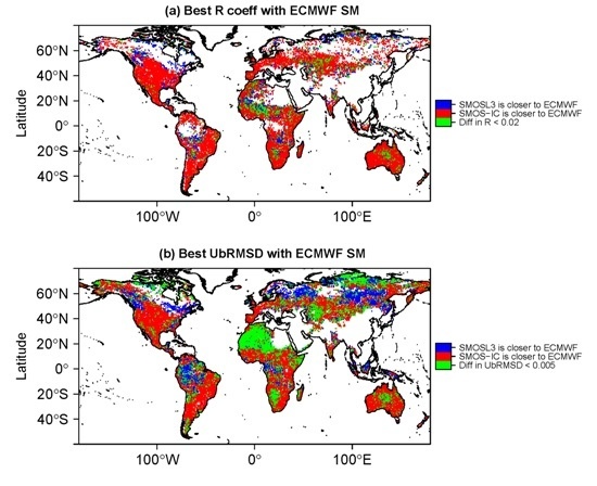
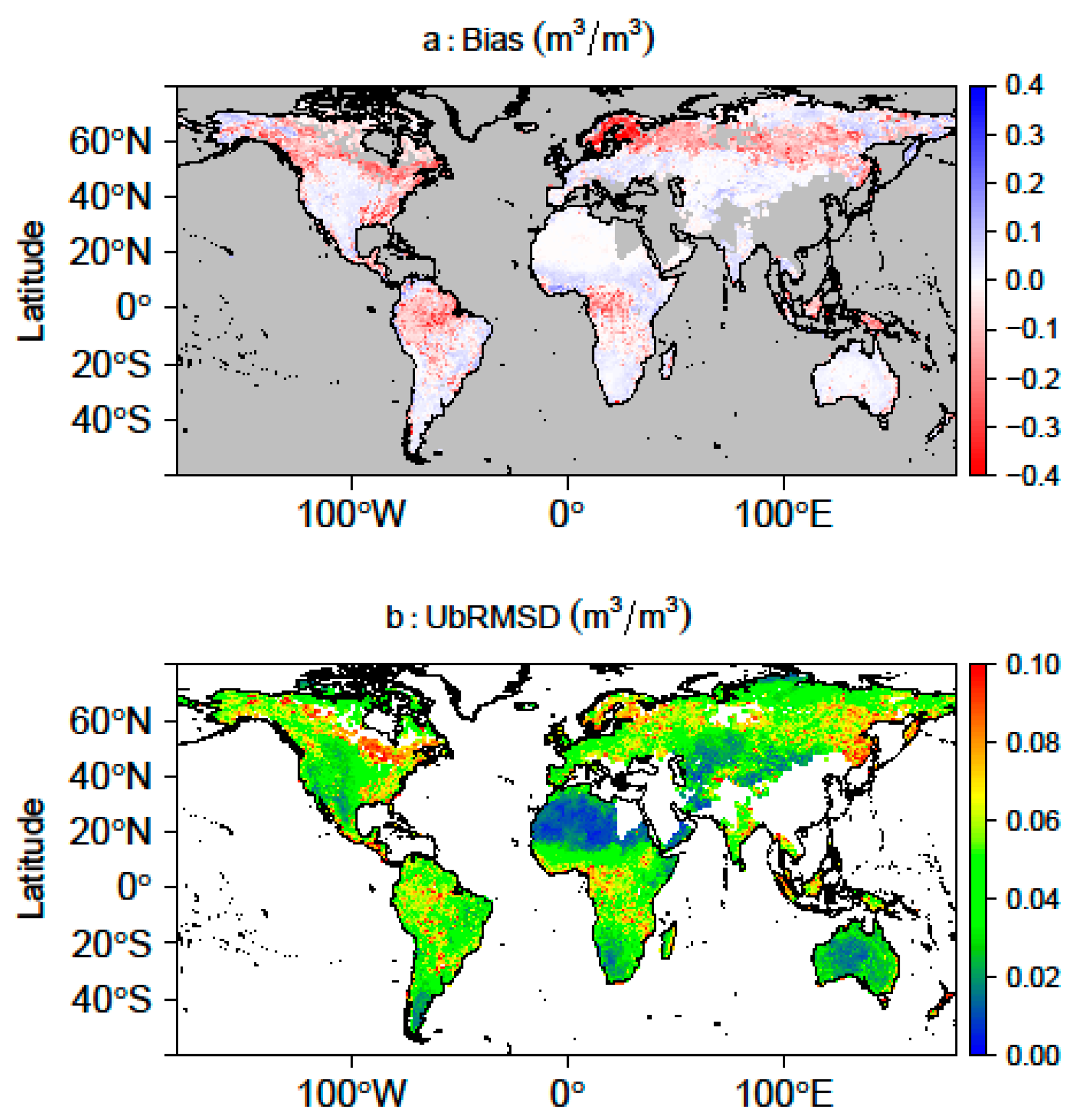
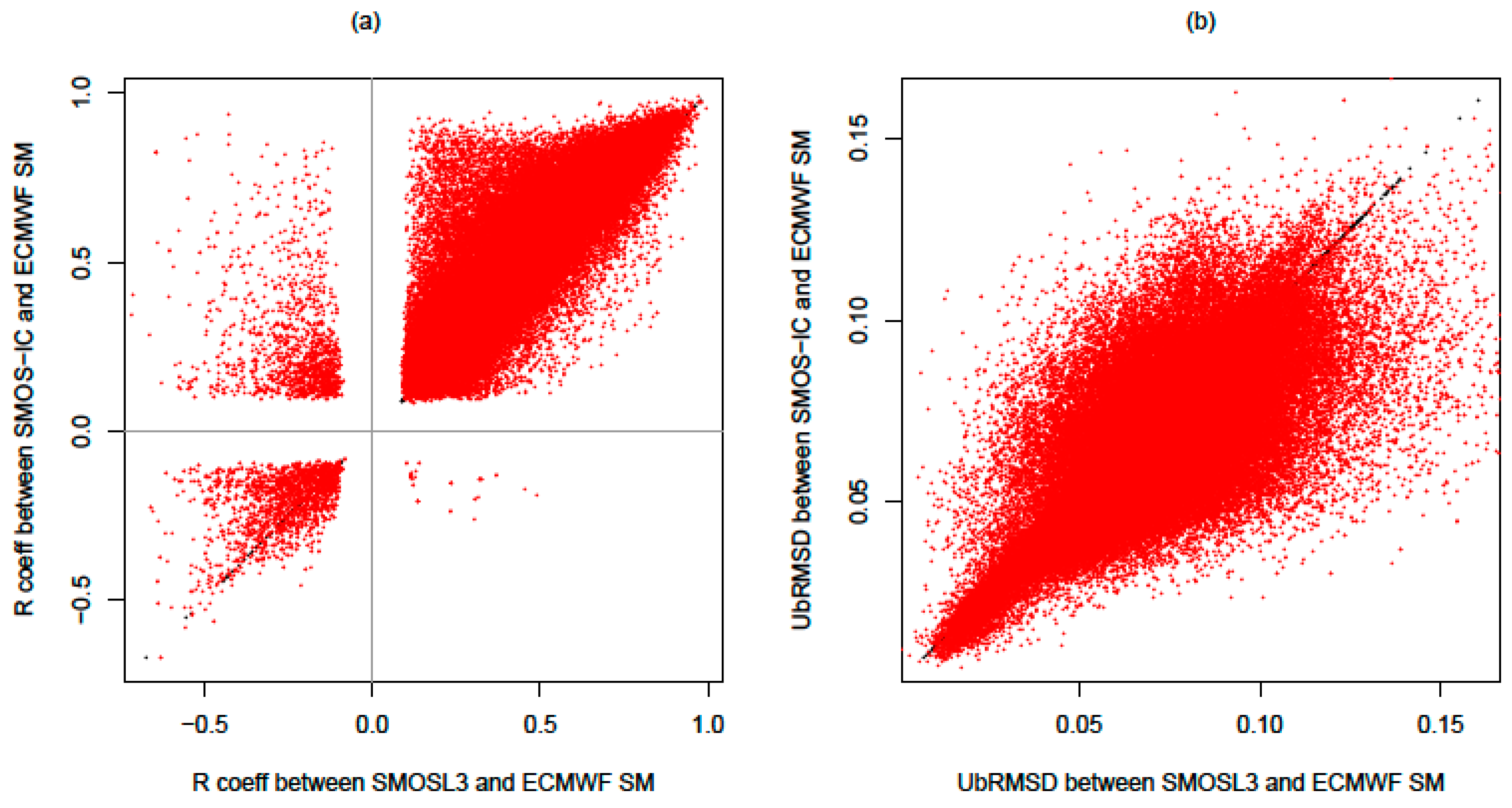
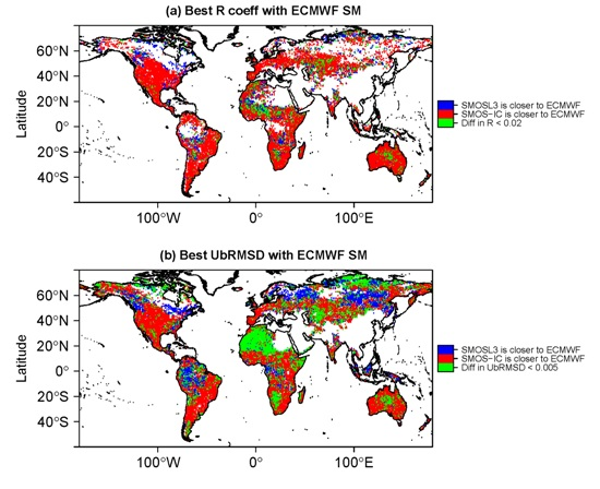
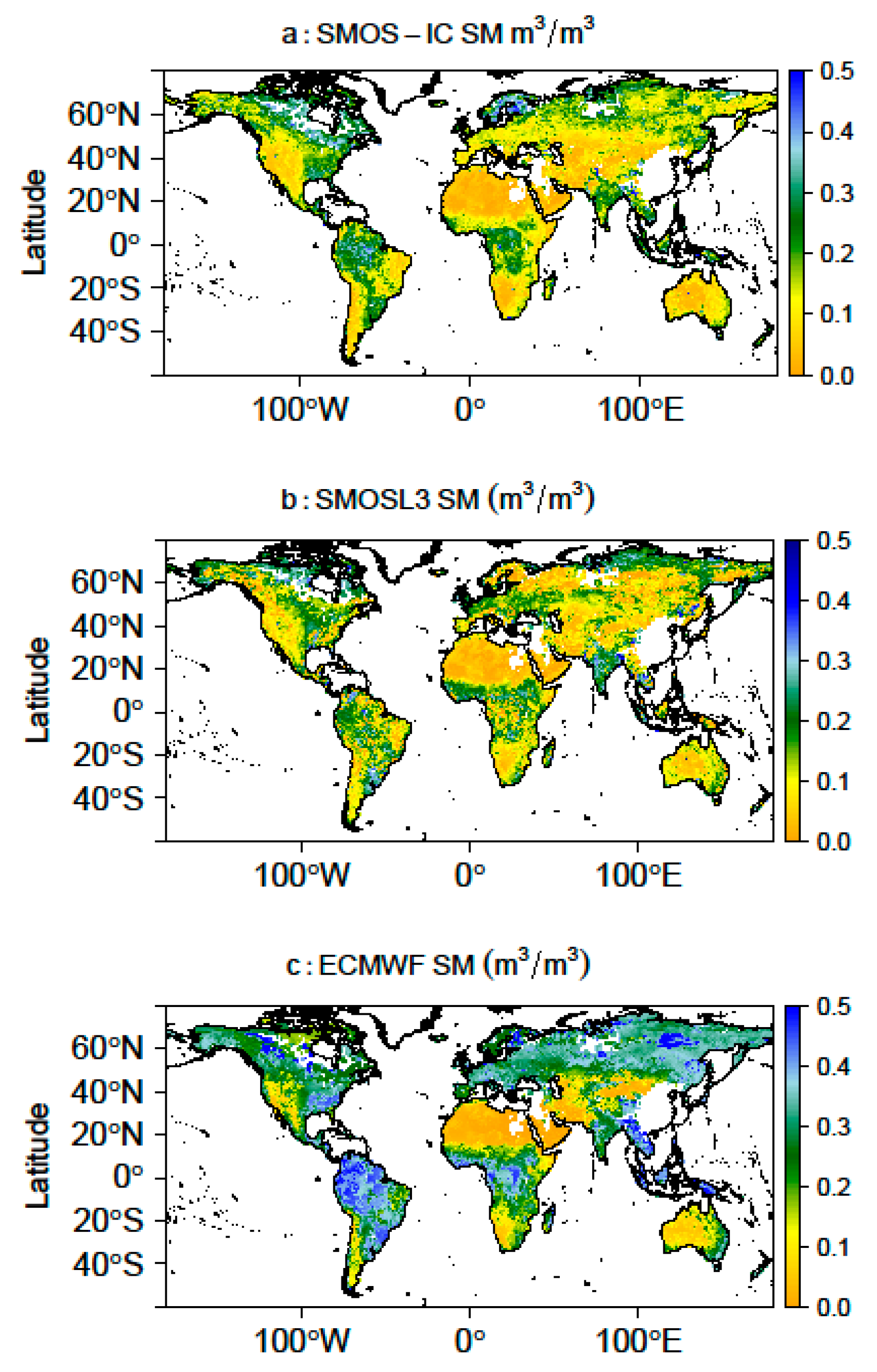
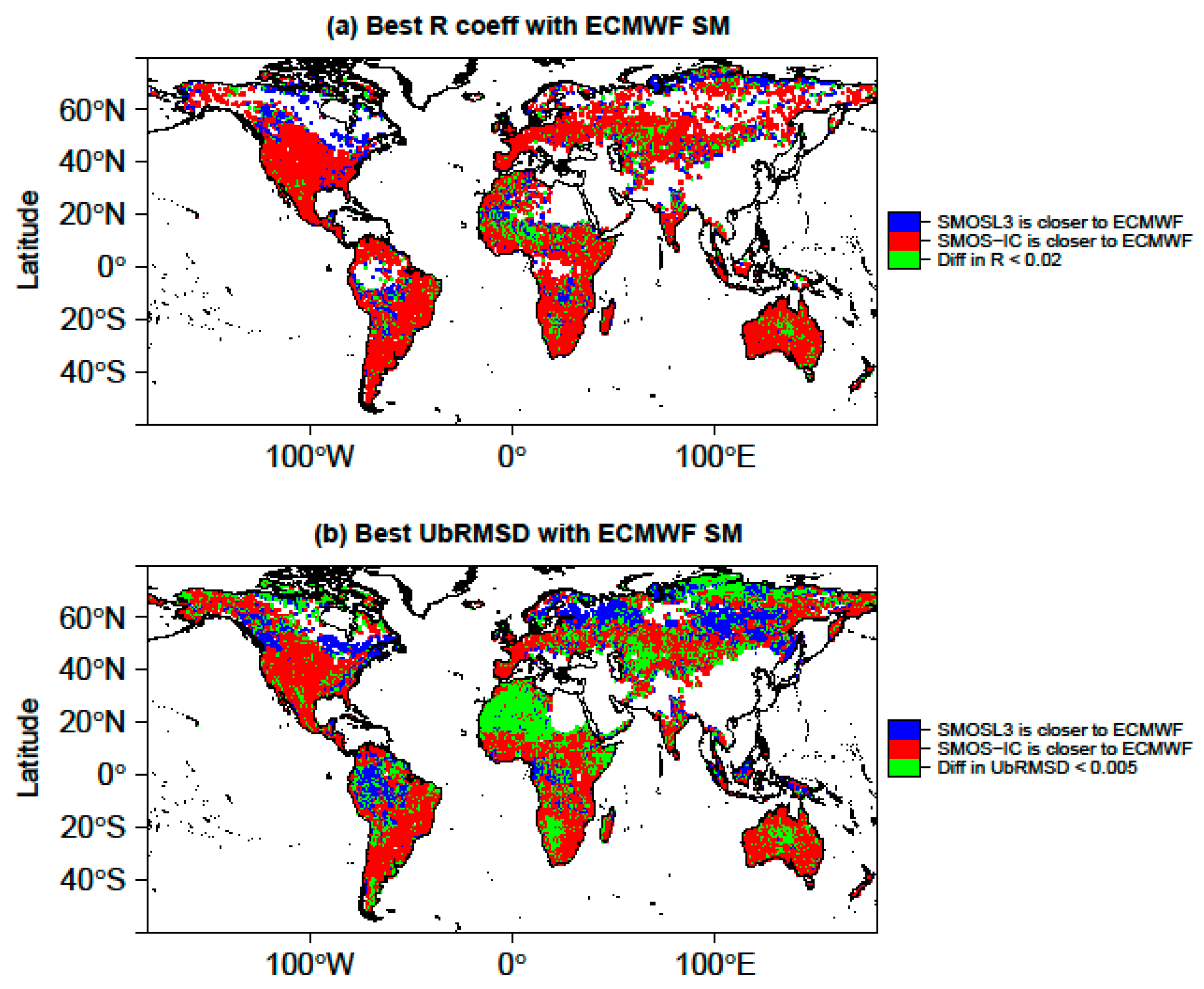
3.1. Soil Moisture

Figure 1 shows the values of the temporal mean SM over the globe and over the period 2010–2015 for the three SM datasets considered in this study: (a) SMOS-IC; (b) SMOSL3 SM; and (c) ECMWF. It should be kept in mind that ECMWF SM is representative of the first 0–7 cm of the soil surface (Albergel et al., 2012 [65]) and the inherent nature of the simulated soil moisture (Koster et al., 2009 [66]) is different to that measured by the SMOS satellite observations, which are sensitive to the first ~0–3 cm of the soil surface (Escorihuela et al., 2010 [67]; Njoku and Kong et al., 1977 [68]). In Figure 1, ECMWF SM must be analyzed in terms of spatial patterns rather than absolute values. Although the images in Figure 1a,b, have many similarities, some spatial patterns shown by the ECMWF SM product are in better agreement with SMOS-IC than with SMOS L3 SM. For instance, over the Appalachian region in the Eastern US, SMOSL3 SM shows a dry area, whereas SMOS-IC SM is closer to ECMWF, as these regions are known to be relatively wetter than the regions of west and midwest (Sheffied et al., 2004 [69]; Fan et al., 2004 [70]). This was partly explained by differences between ECOCLIMAP and IGBP and the use of ECMWF SM data in Mahmoodi et al., 2015 [71]. On the other hand, drier retrievals were found for SMOS-IC in the intertropical regions of Africa, for instance over the savannas and grasslands of Sahel. Over these regions SMOS-L3 SM is closer to ECMWF SM than SMOS-IC SM.

Figure 2 displays different time series metrics derived from the direct comparison between SMOSL3 SM (Figure 2a) and SMOS-IC SM (Figure 2b) with ECMWF SM for 2010–2015. According to correlation (R) results, lowest R values were found in forests for both products. A lower number of negative R values were found between the SMOS-IC and ECMWF SM products. Conversely, SMOSL3 SM yielded negative correlations with ECMWF SM over several forest regions, namely the boreal forests of Alaska, Canada and Russia, and the tropical forests of Amazon and Congo basins. Over the non-forested biomes, R values were also found to be generally higher for SMOS-IC, when compared to SMOSL3 SM. Substantial differences were found in terms of RMSD and ubRMSD. In general, lower values were obtained for the SMOS-IC product, especially over the intertropical regions of America and Africa (in terms of ubRMSD) and the boreal forests of Eurasia (in terms of RMSD). On the other hand, results do not show important differences in terms of bias between the two SMOS products. Both SMOS-IC and SMOSL3 SM products are generally much drier than ECMWF SM, except over some arid and semi-arid areas (deserts in central Asia and Australia, and Sahara in northern Africa) and north of Canada. However, SMOS-IC shows a wet bias in Northern Europe, which cannot be noted for SMOSL3. The general negative values of the bias can be partly explained by the difference between the sampling depth of the SMOS observations (~0–3 cm top soil layer) and the top soil layer considered in the modeled ECMWF SM (0–7 cm top soil layer). Considering this difference, the distinct SM bias patterns shown in Figure 2 should be interpreted with care.

A seasonal statistical analysis that separates cold and warm seasons was carried out and led to similar results to the ones presented above (Figure S1). Figure S1 shows that the ubRMSD is lower in the cold season, i.e., January–March (JFM) in the Northern Hemisphere and July–September (JAS) in the South Hemisphere.

Figure 3 is focused on the results in terms of correlation and ubRMSD, considered as first order criteria. It displays a world map which shows where the best correlation coefficient (R) and ubRMSD are obtained by comparing ECMWF SM with SMOS-IC SM (red) or SMOSL3 SM (blue) in the period 2010–2015. Areas where the result differs by less than 0.02 in terms of R values between SMOSL3 SM and SMOS-IC are represented in green color. This threshold is different for the ubRMSD metric and it was set to 0.005 m³/m³. It can be seen that the red color is dominant, meaning that SMOS-IC SM is generally closer to ECMWF in terms of temporal dynamics but there are some exceptions. For instance, regions colored in blue (SMOSL3 is closer to ECMWF than SMOS-IC) can be found for the ubRMSD metric, in northeastern Europe and northern Asia. It should be noted here that only pixels with significant correlations, i.e., p-value < 0.05 and a number of data >15 are presented.

Figure 4 shows the spatial differences between SMOSL3 and SMOS-IC SM in terms of bias and ubRMSD. It can be observed that the most significant differences for bias were found for forest regions (Amazon and Congo basins, Boreal forests, etc.), where SMOSL3 is drier. In these areas, ubRMSD is also higher, contrary to deserts or barren regions as the Sahara or Central Australia, where the ubRMSD is close to zero.

In order to better assess the range of R and ubRMSD values, the dispersion diagrams displayed in Figure 5 show the scatter plot of both metrics for all pixels and for both SMOS products (SMOS-IC and SMOSL3 SM). In terms of correlation, the R values are generally larger for SMOS-IC. There are also a number of pixels where SMOSL3 SM yields negative correlations, whereas R is positive for SMOS-IC. In terms of ubRMSD, the largest number of pixels with lower ubRMSD corresponds to the SMOS-IC SM product.

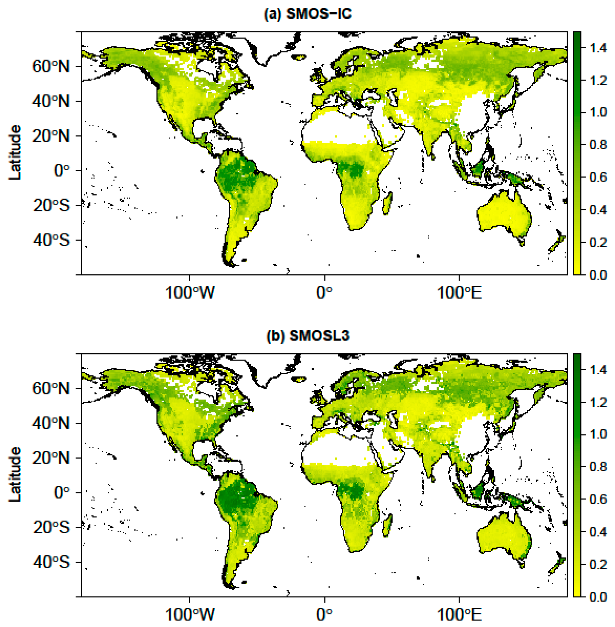
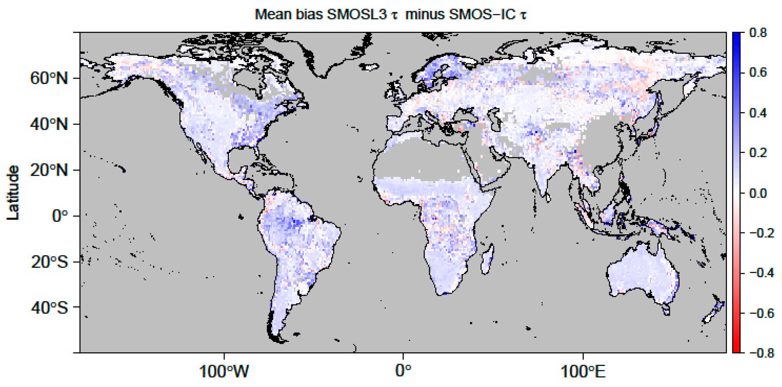
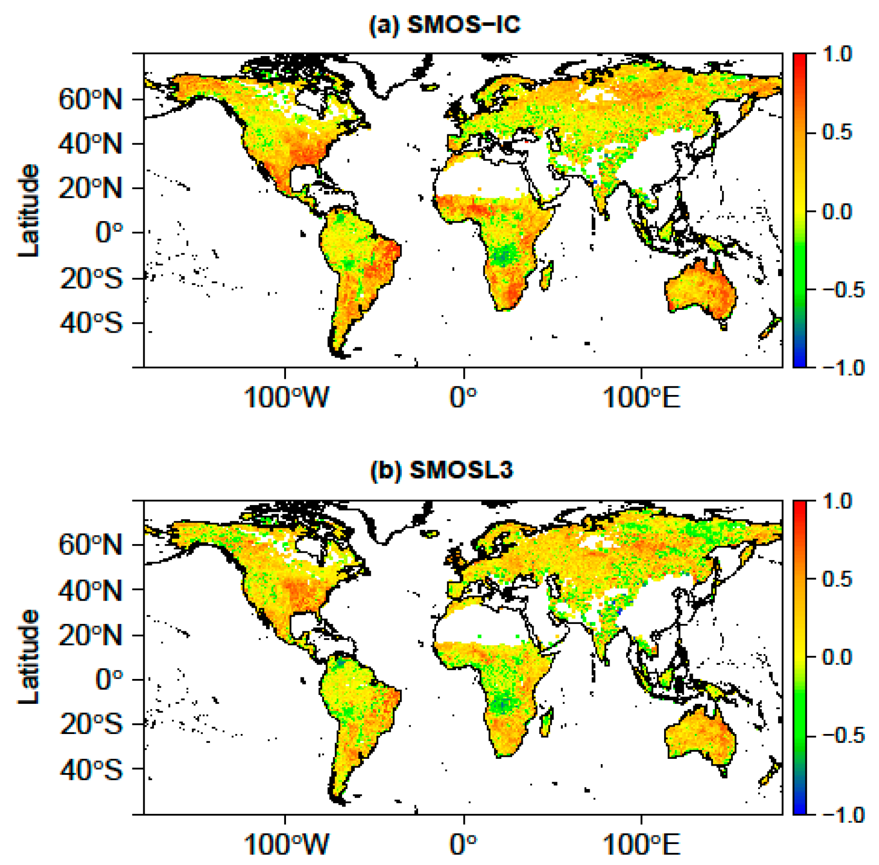
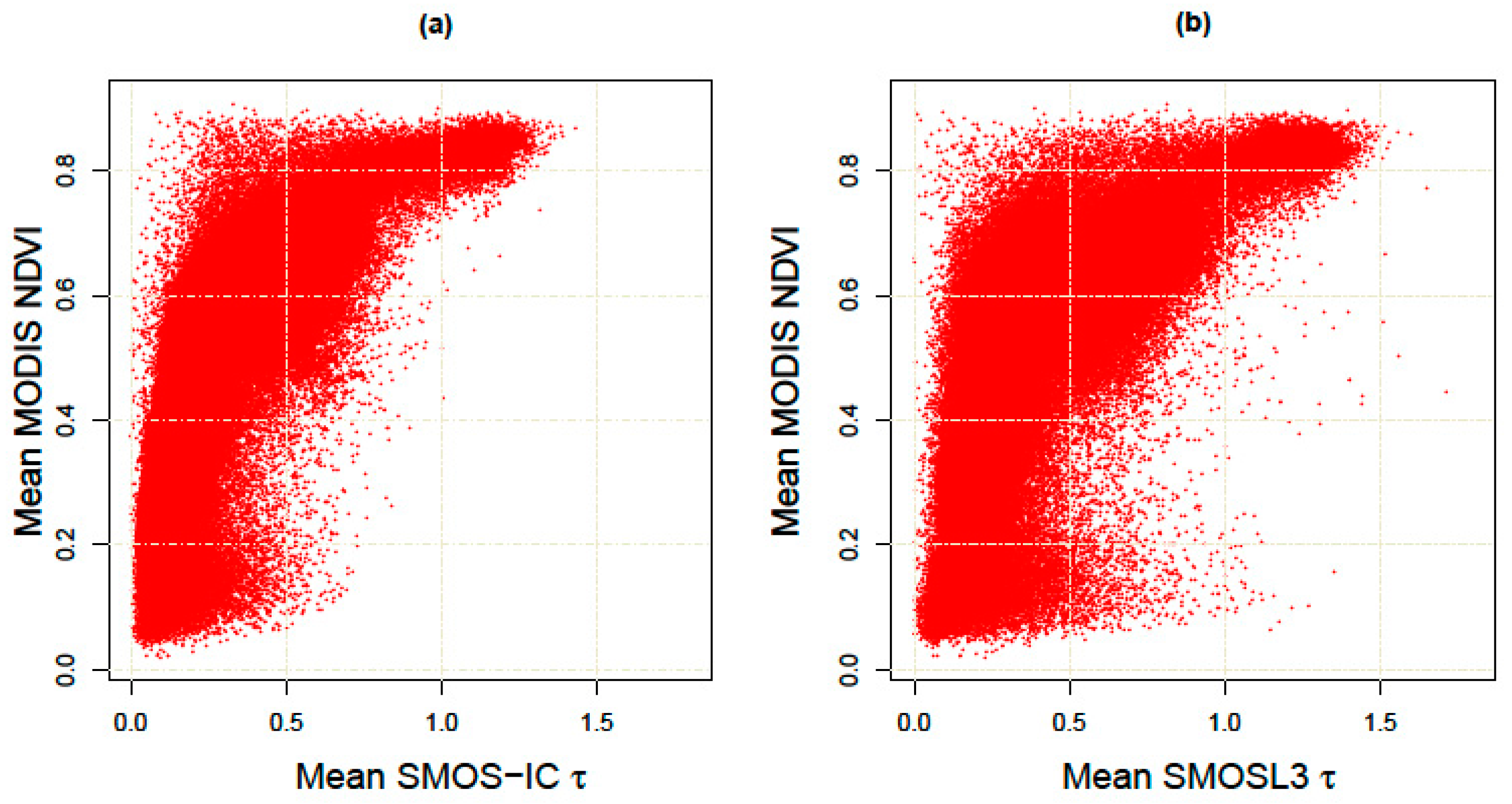
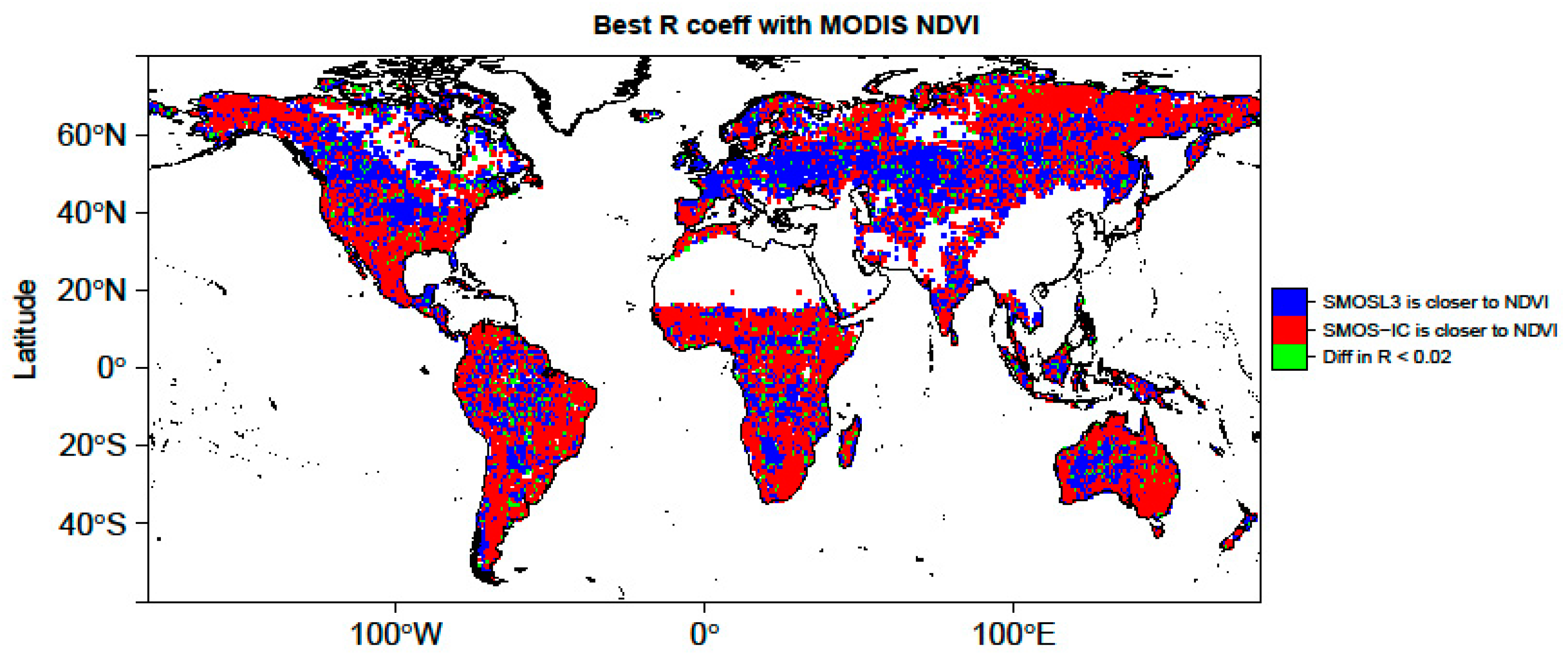
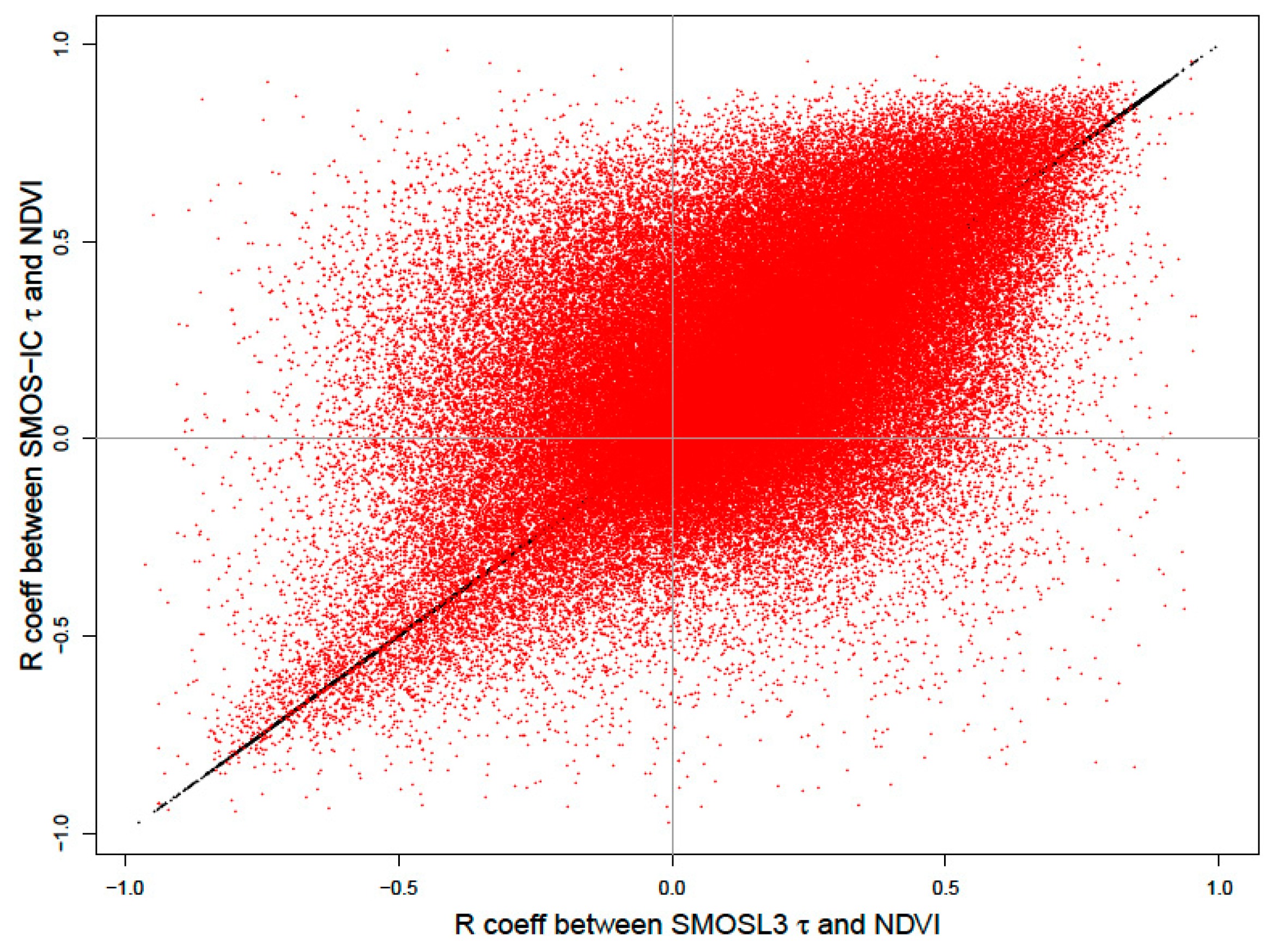
3.2. Vegetation Optical Depth

The evaluation of the accuracy of the τ values retrieved from SMOS at global scale is not a simple issue due to the absence of a consensus on the reference values to be considered at large scale coming from models or in situ measurements. Some studies have been done at local scale. For instance, over croplands and grasslands, τ values at L-band vary generally between 0 and 0.6 (Saleh et al., 2006 [72], Wigneron et al., 2007 [24]). Over forests and from L-band radiometer measurements, Ferrazzoli et al. (2002) [73] found maximum values of τ ~ 0.9, and Grant et al. (2008) [74] found values of τ ~ 0.6–0.7 for a mature pine forest stand in les Landes forest in France, and τ ~ 1 for a mature deciduous (beech) canopy in Switzerland.

Figure 6 shows a global map of the temporal mean of the retrieved τ values for both SMOS-IC and SMOSL3 products. Both products show τ values that are sensitive to vegetation, as the highest τ values were found for the main boreal and tropical forests, and the minimum for dry areas, such as Inner Asia or Australia. It must be noted that the τ values coming from the SMOSL3 product were slightly larger than those obtained by the SMOS-IC product.

In order to identify possible patterns, Figure 7 shows a global map which illustrates the differences of τ between both SMOS datasets (SMOSL3 minus SMOS-IC). This result shows that the greatest differences between both τ datasets were found over some regions of the Northern Hemisphere, such as the east of USA, the north of Europe and also in the Amazon basin.

Figure 8 shows the correlations obtained by comparing the SMOSC-IC and SMOSL3 τ datasets to MODIS NDVI. All correlations values are presented here including those not significant as done by Grant et al. (2016) [25]. It can be noted that slightly higher correlation values are generally obtained with SMOS-IC especially in the west of Mexico, the northeastern regions of Brazil and some parts of the Sahel. Conversely, slightly higher R values were obtained in western and central Europe with SMOSL3. The lowest correlations were found generally over forests for both SMOS products; a result which can be partly related to the tendency of NDVI to saturate for high biomass and LAI values. However, higher R values were obtained with SMOS-IC for some areas of the boreal forests and the tropical forests of Africa.

In order to evaluate how NDVI represents the spatial differences in vegetation density, Figure 9 represents the spatial relation between NDVI and SMOS-IC and SMOSL3 τ. The results demonstrate that there is a general positive trend relating the spatial patterns of τ and NDVI. The latter saturates for values of τ larger than ~0.7. It can be seen that the positive trend relating τ and NDVI is more distinct for SMOS-IC than for SMOSL3.

Figure 10 presents a global map that shows for each pixel which τ dataset (SMOSL3 or SMOS-IC) leads to the largest correlation (R) values with MODIS NDVI. Over northern mid-latitudes, larger correlations were generally obtained with SMOSL3. However, except for these regions, the highest R values were generally obtained with SMOS-IC while no clear patterns were found in terms of longitude. Figure 11 shows a dispersion diagram in order to assess the range of correlation values found for both SMOS τ datasets against MODIS NDVI. The diagram generally yields positive correlations, although a non-negligible number of negative correlations can be noted for both SMOS products. The negative correlation values between τ and NDVI are difficult to explain. In some cases, negative values were found in dense forest areas and can be related to the saturation of NDVI for large biomass values (Grant et al., 2016 [25]).

4. Summary and Conclusions

The main objective of this study is to present an alternative SMOS SM and τ product, referred to as SMOS-IC, and compare it with model data. In terms of soil moisture, the presentation is based on an inter-comparison between SMOS-IC, the official Level 3 SMOS SM product (SMOSL3, V300), and a modeled SM product (ECMWF SM). The SMOS-IC product is based on the retrieval of SM and τ over pixels treated as homogeneous by means of the L-MEB model inversion. SMOS-IC uses the multi-angular and dual-polarization SMOSL3 TB product as the main input for the L-MEB model inversion. The L-MEB model input parameters (effective vegetation scattering albedo ω and the roughness parameter H_R) are estimated as a function of IGBP land category classes which compose the pixel. These parameter values are derived from previous analyses made by Fernandez-Moran et al. (2016) [31] and global maps of the roughness H_R parameter estimated by Parrens et al. (2016) [32]. Conversely, the SMOSL3 product considers different fractions over the pixel and performs SM and τ retrievals over the main fraction of the pixel (usually low vegetation) or over forests in some cases. In the SMOSL3 retrieval algorithm, the TB value of the pixel fraction, which is not considered in the retrieval (the forest fraction in general), is estimated based on auxiliary ECMWF SM data. This specific approach may lead to dry SM bias in forested regions, as noted by Wigneron et al. (2012) [29]. Currently, in the SMOSL3 V300 retrieval algorithm, the values of the vegetation and soil roughness parameters differ mainly between forest and low vegetation categories.

The SMOSL3 and SMOS-IC soil moisture retrievals were compared globally against ECMWF SM data for the period 2010–2015. This evaluation extends the work of Fernandez-Moran et al. (2016) [31] who evaluated a preliminary version of the SMOS-IC product at local scale using numerous in situ SM stations from ISMN and found higher R and lower ubRMSE with SMOS-IC than with the SMOSL3 V300 product. At global scale, both the SMOS-IC and SMOSL3 SM products were generally found to be drier than the ECMWF SM product. However, the different layers considered in the modeled ECMWF SM (top 0–7 cm soil layer) with respect to the remotely sensed SMOS SM (~top 0–3 cm soil layer), as well as the inherently different nature of simulated soil moisture (Koster et al., 2009 [66]), makes it difficult to truly assess the performance of the SMOS products in terms of bias at global scale. In terms of temporal variations, higher correlation values and lower ubRMSD values were generally found between SMOS-IC SM and ECMWF SM, than between SMOSL3 SM and ECMWF SM.

The ECMWF SM dataset is not “truth”, and a larger inter-comparison of SMOS-IC and SMOSL3 against other modeled SM products such as MERRA (Modern-Era Retrospective analysis for Research and Applications) (Reichle et al., 2011 [75]) or remotely sensed data (such as SMAP, AMSR-E, and ASCAT) should be made in the future to confirm the very preliminary results found here. In terms of τ values, the SMOS-IC and SMOSL3 τ products were compared to MODIS NDVI values over 2010–2015 in terms of correlation values. The SMOS-IC τ product presents a slightly lower range of values (~0–1.3) than the one obtained with the SMOSL3 τ product (~0–1.5). These ranges of τ values (obtained for both SMOSL3 and SMOS-IC) are in good agreement with the ranges of retrieved τ values based on in situ L-band radiometric measurements (τ ~0.6–1.0) performed over mature coniferous and deciduous forests in Europe. In general, higher correlation values were obtained between SMOS-IC τ and MODIS NDVI, than between SMOSL3 τ and MODIS NDVI.

The τ results should also be interpreted with care: the NDVI index is derived from optical sensors while the τ index is derived from L-band microwave measurements and therefore can sense deeper through the vegetation canopy. Moreover, the NDVI index is used to monitor the green vegetation, while the τ index is related to the whole vegetation water content (including stems, trunks, branches and senescent vegetation elements). Thus, at L-band, the NDVI index (as the LAI index) is only a proxy, which is used to provide an estimate of τ over rather low vegetation covers during the vegetation growth (O’Neill et al, 2012 [37]; Wigneron et al., 2007 [24]; Lawrence et al., 2014 [76]; Grant et al., 2016 [25]). A larger inter-comparison of the SMOS-IC and SMOSL3 τ products against different vegetation datasets (remotely sensed products, LAI, forest biomass) should be made in the future to confirm the results found in this study.

As for the Level 2 and 3 algorithms, based on rather complex and detailed concepts and auxiliary datasets, the simple SMOS-IC algorithm will be improved regularly and will be used to improve the L2 and L3 SMOS retrieval algorithms. These different approaches are complementary and a regular inter-comparison analysis between them should be of great benefit to improve the L-MEB inversion, and ultimately the SM and τ products retrieved from the SMOS observations.

References

1. Kerr, Y.H.; Waldteufel, P.; Richaume, P.; Wigneron, J.P.; Ferrazzoli, P.; Mahmoodi, A.; Al Bitar, A.; Cabot, F.; Gruhier, C.; Juglea, S.E.; et al. The SMOS Soil Moisture Retrieval Algorithm. Geosci. Remote Sens. 2012, 50, 1384–1403. [Google Scholar] [CrossRef]
2. Entekhabi, D.; Njoku, E.G.; O’Neill, P.E.; Kellogg, K.H.; Crow, W.T.; Edelstein, W.N.; Entin, J.K.; Goodman, S.D.; Jackson, T.J.; Johnson, J.; et al. The soil moisture active passive (SMAP) mission. Proc. IEEE 2010, 98, 704–716. [Google Scholar] [CrossRef]
3. Brocca, L.; Melone, F.; Moramarco, T.; Wagner, W.; Naeimi, V.; Bartalis, Z.; Hasenauer, S. Improving runoff prediction through the assimilation of the ASCAT soil moisture product. Hydrol. Earth Syst. Sci. 2010, 14, 1881–1893. [Google Scholar] [CrossRef]
4. Hollmann, R.; Merchant, C.J.; Saunders, R.; Downy, C.; Buchwitz, M.; Cazenave, A.; Chuvieco, E.; Defourny, P.; De Leeuw, G.; Forsberg, R.; et al. The ESA climate change initiative: Satellite data records for essential climate variables. Bull. Am. Meteorol. Soc. 2013, 94, 1541–1552. [Google Scholar] [CrossRef]
5. Al Bitar, A.; Mialon, A.; Kerr, Y.; Cabot, F.; Richaume, P.; Jacquette, E.; Quesney, A.; Mahmoodi, A.; Tarot, S.; Parrens, M.; et al. The Global SMOS Level 3 daily soil moisture and brightness temperature maps. Earth Syst. Sci. Data Discuss. 2017, in press. [Google Scholar] [CrossRef]
6. Kerr, Y.H.; Waldteufel, P.; Wigneron, J.P.; Martinuzzi, J.M.; Font, J.; Berger, M. Soil moisture retrieval from space: The Soil Moisture and Ocean Salinity (SMOS) mission. IEEE Trans. Geosci. Remote Sens. 2001, 39, 1729–1735. [Google Scholar] [CrossRef]
7. Mialon, A.; Richaume, P.; Leroux, D.; Bircher, S.; Al Bitar, A.; Pellarin, T.; Wigneron, J.P.; Kerr, Y.H. Comparison of Dobson and Mironov dielectric models in the SMOS soil moisture retrieval algorithm. IEEE Trans. Geosci. Remote Sens. 2015, 53, 3084–3094. [Google Scholar] [CrossRef]
8. Al-Yaari, A.; Wigneron, J.P.; Ducharne, A.; Kerr, Y.H.; Wagner, W.; De Lannoy, G.; Reichle, R.; Al Bitar, A.; Dorigo, W.; Richaume, P.; et al. Global-scale comparison of passive (SMOS) and active (ASCAT) satellite based microwave soil moisture retrievals with soil moisture simulations (MERRA-Land). Remote Sens. Environ. 2014, 152, 614–626. [Google Scholar] [CrossRef]
9. Al-Yaari, A.; Wigneorn, J.P.; Ducharne, A.; Kerr, Y.; Fernandez-Moran, R.; Parrens, M.; Al Bitar, A.; Mialon, A.; Richaume, P. Evaluation of the most recent reprocessed SMOS soil moisture products: Comparison between SMOS level 3 V246 and V272. In Proceedings of the 2015 IEEE International Geoscience and Remote Sensing Symposium (IGARSS), Milan, Italy, 26–31 July 2015. [Google Scholar]
10. Al-Yaari, A.; Wigneron, J.-P.; Kerr, Y.; Rodriguez-Fernandez, N.; O’Neill, P.E.; Jackson, T.J.; De Lannoy, G.J.M.; Al Bitar, A.; Mialon, A.; Richaume, P.; et al. Evaluating soil moisture retrievals from ESA’s SMOS and NASA’s SMAP brightness temperature datasets. Remote Sens. Environ. 2017, 193, 257–273. [Google Scholar] [CrossRef]
11. Kerr, Y.H.; Al-Yaari, A.; Rodriguez-Fernandez, N.; Parrens, M.; Molero, B.; Leroux, D.; Bircher, S.; Mahmoodi, A.; Mialon, A.; Richaume, P.; et al. Overview of SMOS performance in terms of global soil moisture monitoring after six years in operation. Remote Sens. Environ. 2016, 180, 40–63. [Google Scholar] [CrossRef]
12. Wigneron, J.-P.; Jackson, T.J.; O’Neill, P.; De Lannoy, G.; de Rosnay, P.; Walker, J.P.; Ferrazzoli, P.; Mironov, V.; Bircher, S.; Grant, J.P.; et al. Modelling the passive microwave signature from land surfaces: A review of recent results and application to the L-band SMOS & SMAP soil moisture retrieval algorithms. Remote Sens. Environ. 2017, 192, 238–262. [Google Scholar]
13. Rahmoune, R.; Ferrazzoli, P.; Kerr, Y.H.; Richaume, P. SMOS level 2 retrieval algorithm over forests: Description and generation of global maps. IEEE J. Sel. Top. Appl. Earth Obs. Remote Sens. 2013, 6, 1430–1439. [Google Scholar] [CrossRef]
14. Rahmoune, R.; Ferrazzoli, P.; Singh, Y.K.; Kerr, Y.H.; Richaume, P.; Al Bitar, A. SMOS retrieval results over forests: Comparisons with independent measurements. IEEE J. Sel. Top. Appl. Earth Obs. Remote Sens. 2014, 7, 3858–3866. [Google Scholar] [CrossRef]
15. Schwank, M.; Mätzler, C.; Guglielmetti, M.; Flühler, H. L-band radiometer measurements of soil water under growing clover grass. IEEE Trans. Geosci. Remote Sens. 2005, 43, 2225–2236. [Google Scholar] [CrossRef]
16. Schwank, M.; Wigneron, J.P.; López-Baeza, E.; Völksch, I.; Mätzler, C.; Kerr, Y.H. L-band radiative properties of vine vegetation at the MELBEX III SMOS cal/val site. IEEE Trans. Geosci. Remote Sens. 2012, 50, 1587–1601. [Google Scholar] [CrossRef]
17. Jackson, T.J.; Schmugge, T.J. Vegetation effects on the microwave emission of soils. Remote Sens. Environ. 1991, 36, 203–212. [Google Scholar] [CrossRef]
18. Mo, T.; Choudhury, B.J.; Schmugge, T.J.; Wang, J.R.; Jackson, T.J. A model for microwave emission from vegetation-covered fields. J. Geophys. Res. 1982, 87, 11229. [Google Scholar] [CrossRef]
19. Wigneron, J.P.; Chanzy, A.; Calvet, J.C.; Bruguier, N. A simple algorithm to retrieve soil moisture and vegetation biomass using passive microwave measurements over crop fields. Remote Sens. Environ. 1995, 51, 331–341. [Google Scholar] [CrossRef]
20. Grant, J.P.; Wigneron, J.P.; Drusch, M.; Williams, M.; Law, B.E.; Novello, N.; Kerr, Y. Investigating temporal variations in vegetation water content derived from SMOS optical depth. In Proceedings of the 2012 IEEE International Geoscience and Remote Sensing Symposium (IGARSS), Munich, Germany, 22–27 July 2012. [Google Scholar]
21. Schneebeli, M.; Wolf, S.; Kunert, N.; Eugster, W.; Mätzler, C. Relating the X-band opacity of a tropical tree canopy to sapflow, rain interception and dew formation. Remote Sens. Environ. 2011, 115, 2116–2125. [Google Scholar] [CrossRef]
22. Guglielmetti, M.; Schwank, M.; Mätzler, C.; Oberdörster, C.; Vanderborght, J.; Flühler, H. FOSMEX: Forest soil moisture experiments with microwave radiometry. IEEE Trans. Geosci. Remote Sens. 2008, 46, 727–735. [Google Scholar] [CrossRef]
23. Patton, J.; Member, S.; Hornbuckle, B. Initial validation of smos vegetation optical thickness in Iowa. IEEE Geosci. Remote Sens. Lett. 2013, 10, 647–651. [Google Scholar] [CrossRef]
24. Wigneron, J.P.; Kerr, Y.; Waldteufel, P.; Saleh, K.; Escorihuela, M.J.; Richaume, P.; Ferrazzoli, P.; de Rosnay, P.; Gurney, R.; Calvet, J.C.; et al. L-band microwave emission of the biosphere (L-MEB) model: Description and calibration against experimental data sets over crop fields. Remote Sens. Environ. 2007, 107, 639–655. [Google Scholar] [CrossRef]
25. Grant, J.P.; Wigneron, J.P.; De Jeu, R.A.M.; Lawrence, H.; Mialon, A.; Richaume, P.; Al Bitar, A.; Drusch, M.; van Marle, M.J.E.; Kerr, Y.; et al. Comparison of SMOS and AMSR-E vegetation optical depth to four MODIS-based vegetation indices. Remote Sens. Environ. 2016, 172, 87–100. [Google Scholar] [CrossRef]
26. Fernandez-Moran, R.; Wigneron, J.-P.; Lopez-Baeza, E.; Al-Yaari, A.; Bircher, S.; Coll-Pajaron, A.; Mahmoodi, A.; Parrens, M.; Richaume, P.; Kerr, Y. Analyzing the impact of using the SRP (Simplified roughness parameterization) method on soil moisture retrieval over different regions of the globe. In Proceedings of the 2015 IEEE International Geoscience and Remote Sensing Symposium (IGARSS), Milan, Italy, 26–31 July 2015. [Google Scholar]
27. Parrens, M.; Wigneron, J.-P.; Richaume, P.; Al Bitar, A.; Mialon, A.; Fernandez-Moran, R.; Al-Yaari, A.; O’Neill, P.; Kerr, Y. Considering combined or separated roughness and vegetation effects in soil moisture retrievals. Int. J. Appl. Earth Obs. Geoinf. 2017, 55, 73–86. [Google Scholar] [CrossRef]
28. Wigneron, J.P.; Chanzy, A.; Kerr, Y.H.; Lawrence, H.; Shi, J.; Escorihuela, M.J.; Mironov, V.; Mialon, A.; Demontoux, F.; De Rosnay, P.; et al. Evaluating an improved parameterization of the soil emission in L-MEB. IEEE Trans. Geosci. Remote Sens. 2011, 49, 1177–1189. [Google Scholar] [CrossRef]
29. Wigneron, J.P.; Schwank, M.; Baeza, E.L.; Kerr, Y.; Novello, N.; Millan, C.; Moisy, C.; Richaume, P.; Mialon, A.; Al Bitar, A.; et al. First evaluation of the simultaneous SMOS and ELBARA-II observations in the Mediterranean region. Remote Sens. Environ. 2012, 124, 26–37. [Google Scholar] [CrossRef]
30. Kaufman, Y.J.; Justice, C.O.; Flynn, L.P.; Kendall, J.D.; Prins, E.M.; Giglio, L.; Ward, D.E.; Menzel, W.P.; Setzer, A.W. Potential global fire monitoring from EOS-MODIS. J. Geophys. Res. 1998, 103, 32215–32238. [Google Scholar] [CrossRef]
31. Fernandez-Moran, R.; Wigneron, J.-P.; De Lannoy, G.; Lopez-Baeza, E.; Mialon, A.; Mahmoodi, A.; Parrens, M.; Al Bitar, A.; Richaume, P.; Kerr, Y. Calibrating the effective scattering albedo in the SMOS algorithm: Some first results. In Proceedings of the 2016 IEEE International Geoscience and Remote Sensing Symposium (IGARSS), Beijing, China, 10–16 July 2016. [Google Scholar]
32. Parrens, M.; Wigneron, J.P.; Richaume, P.; Mialon, A.; Al Bitar, A.; Fernandez-Moran, R.; Al-Yaari, A.; Kerr, Y.H. Global-scale surface roughness effects at L-band as estimated from SMOS observations. Remote Sens. Environ. 2016, 181, 122–136. [Google Scholar] [CrossRef]
33. Rouse, J.W.; Haas, R.H.; Schell, J.A. Monitoring the Vernal Advancement and Retrogradation (Greenwave Effect) of Natural Vegetation; NASA Goddard Space Flight Center: Texas, TX, USA, 1974; pp. 1–8.
34. Guglielmetti, M.; Schwank, M.; Mätzler, C.; Oberdörster, C.; Vanderborght, J.; Flühler, H. Measured microwave radiative transfer properties of a deciduous forest canopy. Remote Sens. Environ. 2007, 109, 523–532. [Google Scholar] [CrossRef]
35. Santi, E.; Paloscia, S.; Pampaloni, P.; Pettinato, S. Ground-based microwave investigations of forest plots in Italy. IEEE Trans. Geosci. Remote Sens. 2009, 47, 3016–3025. [Google Scholar] [CrossRef]
36. Qi, J.; Chehbouni, A.; Huete, A.R.; Kerr, Y.H.; Sorooshian, S. A modified soil adjusted vegetation index. Remote Sens. Environ. 1994, 48, 119–126. [Google Scholar] [CrossRef]
37. O’Neill, P.; Chan, S.; Njoku, E.; Jackson, T.; Bindlish, R. Soil Moisture Active Passive (SMAP) Algorithm Theoretical Basis Document (ATBD). SMAP Level 2 & 3 Soil Moisture (Passive), (L2_SM_P, L3_SM_P); JPL: Pasadena, CA, USA, 2012. [Google Scholar]
38. Corbella, I.; Torres, F.; Duffo, N.; González-Gambau, V.; Pablos, M.; Duran, I.; Martín-Neira, M. MIRAS calibration and performance: Results from the SMOS in-orbit commissioning phase. IEEE Trans. Geosci. Remote Sens. 2011, 49, 3147–3155. [Google Scholar] [CrossRef]
39. Armstrong, R.; Brodzik, M.J.; Varani, A. The NSIDC EASE-Grid: Addressing the need for a common, flexible, mapping and gridding scheme. Earth Syst. Monit. 1997, 7, 6–7. [Google Scholar]
40. A Versatile Set of Equal-Area Projections and Grids. Available online: http://www.ncgia.ucsb.edu/globalgrids-book/ease_grid/ (accessed on 5 May 2017).
41. Kerr, Y.; Jacquette, E.; Al Bitar, A.; Cabot, F.; Mialon, A.; Richaume, P.; Quesney, A.; Berthon, L. CATDS SMOS L3 Soil Moisture Retrieval Processor Algorithm Theoretical Baseline Document (ATBD); CESBIO: Toulouse, France, 2013. [Google Scholar]
42. Jacquette, E.; Al Bitar, A.; Mialon, A.; Kerr, Y.; Quesney, A.; Cabot, F.; Richaume, P. SMOS CATDS level 3 global products over land. Proc. SPIE 2016. [Google Scholar] [CrossRef]
43. Oliva, R.; Daganzo-Eusebio, E.; Kerr, Y.H.; Mecklenburg, S.; Nieto, S.; Richaume, P.; Gruhier, C. SMOS radio frequency interference scenario: Status and actions taken to improve the RFI environment in the 1400–1427-MHZ passive band. IEEE Trans. Geosci. Remote Sens. 2012, 50, 1427–1439. [Google Scholar] [CrossRef]
44. Khazaal, A.; Anterrieu, E.; Cabot, F.; Kerr, Y.H. Impact of Direct Solar Radiations Seen by the Back-Lobes Antenna Patterns of SMOS on the Retrieved Images. IEEE J. Sel. Top. Appl. Earth Obs. Remote Sens. 2016, PP, 1–8. [Google Scholar] [CrossRef]
45. Wang, J.R.; Choudhury, B.J. Remote sensing of soil moisture content, over bare field at 1.4 GHz frequency. J. Geophys. Res. 1981, 86, 5277–5282. [Google Scholar] [CrossRef]
46. Escorihuela, M.J.; Kerr, Y.H.; De Rosnay, P.; Wigneron, J.P.; Calvet, J.C.; Lemaître, F. A simple model of the bare soil microwave emission at L-band. IEEE Trans. Geosci. Remote Sens. 2007, 45, 1978–1987. [Google Scholar] [CrossRef]
47. Lawrence, H.; Wigneron, J.-P.; Demontoux, F.; Mialon, A.; Kerr, Y.H. Evaluating the Semiempirical H-Q Model Used to Calculate the L-Band Emissivity of a Rough Bare Soil. IEEE Trans. Geosci. Remote Sens. 2013, 51, 4075–4084. [Google Scholar] [CrossRef]
48. Ulaby, F.T.; Moore, R.K.; Fung, A.K. Microwave Remote Sensing Active and Passive Volume II: Radar Remote Sensing and Surface Scattering and Emission Theory; Addison Wesley: New York, NY, USA, 1982; Volume 2. [Google Scholar]
49. Mironov, V.; Kerr, Y.; Member, S.; Wigneron, J.; Member, S. Temperature- and Texture-Dependent Dielectric Model for Moist Soils at 1.4 GHz. IEEE Geosci. Remote Sens. Lett. 2012, 10, 1–5. [Google Scholar] [CrossRef]
50. Fernandez-Moran, R.; Wigneron, J.P.; Lopez-Baeza, E.; Al-Yaari, A.; Coll-Pajaron, A.; Mialon, A.; Miernecki, M.; Parrens, M.; Salgado-Hernanz, P.M.; Schwank, M.; et al. Roughness and vegetation parameterizations at L-band for soil moisture retrievals over a vineyard field. Remote Sens. Environ. 2015, 170, 269–279. [Google Scholar] [CrossRef]
51. Masson, V.; Champeaux, J.L.; Chauvin, F.; Meriguet, C.; Lacaze, R. A global database of land surface parameters at 1-km resolution in meteorological and climate models. J. Clim. 2003, 16, 1261–1282. [Google Scholar] [CrossRef]
52. FAO; UNESCO. Soil Map of the World, Revised Legend; Food and Agriculture Organization of the United Nations: Rome, Italy, 1988. [Google Scholar]
53. Berrisford, P.; Kållberg, P.; Kobayashi, S.; Dee, D.; Uppala, S.; Simmons, A.J.; Poli, P.; Sato, H. Atmospheric conservation properties in ERA-Interim. Q. J. R. Meteorol. Soc. 2011, 137, 1381–1399. [Google Scholar] [CrossRef]
54. Wigneron, J.-P.; Laguerre, L.; Kerr, Y.H. A simple parameterization of the L-band microwave emission from rough agricultural soils. IEEE Trans. Geosci. Remote Sens. 2001, 39, 1697–1707. [Google Scholar] [CrossRef]
55. Al-Yaari, A.; Wigneron, J.P.; Ducharne, A.; Kerr, Y.; de Rosnay, P.; de Jeu, R.; Govind, A.; Al Bitar, A.; Albergel, C.; Muñoz-Sabater, J.; et al. Global-scale evaluation of two satellite-based passive microwave soil moisture datasets (SMOS and AMSR-E) with respect to Land Data Assimilation System estimates. Remote Sens. Environ. 2014, 149, 181–195. [Google Scholar] [CrossRef]
56. Albergel, C.; Dorigo, W.; Balsamo, G.; Muñoz-Sabater, J.; de Rosnay, P.; Isaksen, L.; Brocca, L.; de Jeu, R.; Wagner, W. Monitoring multi-decadal satellite earth observation of soil moisture products through land surface reanalyses. Remote Sens. Environ. 2013, 138, 77–89. [Google Scholar] [CrossRef]
57. Leroux, D.J.; Kerr, Y.H.; Al Bitar, A.; Bindlish, R.; Member, S.; Jackson, T.J.; Berthelot, B.; Portet, G. Comparison Between SMOS, VUA, ASCAT, and ECMWF soil moisture products over four watersheds in US. IEEE Trans. Geos. Remote Sens. 2014, 52, 1562–1571. [Google Scholar] [CrossRef]
58. Albergel, C.; de Rosnay, P.; Gruhier, C.; Muñoz-Sabater, J.; Hasenauer, S.; Isaksen, L.; Kerr, Y.; Wagner, W. Evaluation of remotely sensed and modelled soil moisture products using global ground-based in situ observations. Remote Sens. Environ. 2012, 118, 215–226. [Google Scholar] [CrossRef]
59. Louvet, S.; Pellarin, T.; Al Bitar, A.; Cappelaere, B.; Galle, S.; Grippa, M.; Gruhier, C.; Kerr, Y.; Lebel, T.; Mialon, A.; et al. SMOS soil moisture product evaluation over West-Africa from local to regional scale. Remote Sens. Environ. 2015, 156, 383–394. [Google Scholar] [CrossRef]
60. De Jeu, R.A.M.; Owe, M. Further validation of a new methodology for surface moisture and vegetation optical depth retrieval. Int. J. Remote Sens. 2003, 24, 4559–4578. [Google Scholar] [CrossRef]
61. Andela, N.; Liu, Y.Y.; Van Dijk, A.I.J.M.; De Jeu, R.A.M.; McVicar, T.R. Global changes in dryland vegetation dynamics (1988-2008) assessed by satellite remote sensing: Comparing a new passive microwave vegetation density record with reflective greenness data. Biogeosciences 2013, 10, 6657–6676. [Google Scholar] [CrossRef]
62. Tian, F.; Brandt, M.; Liu, Y.Y.; Rasmussen, K.; Fensholt, R. Mapping gains and losses in woody vegetation across global tropical drylands. Glob. Chang. Biol. 2016, 23, 1748–1760. [Google Scholar] [CrossRef] [PubMed]
63. Tian, F.; Brandt, M.; Liu, Y.Y.; Verger, A.; Tagesson, T.; Diouf, A.A.; Rasmussen, K.; Mbow, C.; Wang, Y.; Fensholt, R. Remote sensing of vegetation dynamics in drylands: Evaluating vegetation optical depth (VOD) using AVHRR NDVI and in situ green biomass data over West African Sahel. Remote Sens. Environ. 2016, 177, 265–276. [Google Scholar] [CrossRef]
64. Dorigo, W.A.; Xaver, A.; Vreugdenhil, M.; Gruber, A.; Hegyiová, A.; Sanchis-Dufau, A.D.; Zamojski, D.; Cordes, C.; Wagner, W.; Drusch, M. Global Automated Quality Control of In Situ Soil Moisture Data from the International Soil Moisture Network. Vadose Zone J. 2013. [Google Scholar] [CrossRef]
65. Albergel, C.; de Rosnay, P.; Balsamo, G.; Isaksen, L.; Muñoz-Sabater, J. Soil moisture analyses at ECMWF: evaluation using global ground-based in situ observations. J. Hydrometeorol. 2012, 13, 1442–1460. [Google Scholar] [CrossRef]
66. Koster, R.D.; Guo, Z.C.; Yang, R.Q.; Dirmeyer, P.A.; Mitchell, K.; Puma, M.J. On the Nature of Soil Moisture in Land Surface Models. J. Clim. 2009, 22, 4322–4335. [Google Scholar] [CrossRef]
67. Escorihuela, M.J.; Chanzy, A.; Wigneron, J.P.; Kerr, Y.H. Effective soil moisture sampling depth of L-band radiometry: A case study. Remote Sens. Environ. 2010, 114, 995–1001. [Google Scholar] [CrossRef]
68. Njoku, E.G.; Kong, J.-A. Theory for passive microwave remote sensing of near-surface soil moisture. J. Geophys. Res. 1977, 82, 3108–3118. [Google Scholar] [CrossRef]
69. Sheffield, J.; Goteti, G.; Wen, F.; Wood, E.F. A simulated soil moisture based drought analysis for the United States. J. Geophys. Res. D Atmos. 2004, 109, 1–19. [Google Scholar] [CrossRef]
70. Fan, Y.; van den Dool, H. Climate prediction center global monthly soil moisture data set at 0.5° resolution for 1948 to present. J. Geophys. Res. D Atmos. 2004, 109, D10102. [Google Scholar] [CrossRef]
71. Mahmoodi, A.; Richaume, P.; Kerr, Y.; Mialon, A.; Bircher, S.; Leroux, D. Evaluation of MODIS IGBP land cover data on the SMOS Level 2 soil soisture retrievals. In Proceedings of the 2nd SMOS Science Conference, Madrid, Spain, 25–29 May 2015. [Google Scholar]
72. Saleh, K.; Wigneron, J.P.; De Rosnay, P.; Calvet, J.C.; Kerr, Y. Semi-empirical regressions at L-band applied to surface soil moisture retrievals over grass. Remote Sens. Environ. 2006, 101, 415–426. [Google Scholar] [CrossRef]
73. Ferrazzoli, P.; Guerriero, L.; Wigneron, J.P. Simulating L-band emission of forests in view of future satellite applications. IEEE Trans. Geosci. Remote Sens. 2002, 40, 2700–2708. [Google Scholar] [CrossRef]
74. Grant, J.P.; Saleh-Contell, K.; Wigneron, J.-P.; Guglielmetti, M.; Kerr, Y.H.; Schwank, M.; Skou, N.; Van de Griend, A. Calibration of the L-MEB model over a conniferous and a deciduous forest. IEEE Trans. Geosci. Remote Sens. 2008, 46, 808–818. [Google Scholar] [CrossRef]
75. Reichle, R.H.; Koster, R.D.; De Lannoy, G.J.M.; Forman, B.A.; Liu, Q.; Mahanama, S.P.P.; Toure, A. Assessment and enhancement of MERRA land surface hydrology estimates. J. Clim. 2011, 24, 6322–6338. [Google Scholar] [CrossRef]
76. Lawrence, H.; Wigneron, J.P.; Richaume, P.; Novello, N.; Grant, J.; Mialon, A.; Al Bitar, A.; Merlin, O.; Guyon, D.; Leroux, D.; et al. Comparison between SMOS Vegetation Optical Depth products and MODIS vegetation indices over crop zones of the USA. Remote Sens. Environ. 2014, 140, 396–406. [Google Scholar] [CrossRef]
Figure 1. Temporal mean of soil moisture (m3/m3) during 2010–2015: (a) SMOS-IC (SMOS-INRA-CESBIO); (b) SMOSL3 SM (Level 3 SMOS soil moisture); and (c) ECMWF (European Center for Medium range Weather Forecasting) data. White values mean “no valid SMOS data”.
Remotesensing 09 00457 g001
Figure 2. Pixel-based statistics during 2010–2015 computed between ECMWF SM simulations and: SMOSL3 SM (left); and SMOS-IC (right) SM retrievals: (a,b) correlation coefficient; (c,d) Root Mean Square Deviation (RMSD); (e,f) bias; and (g,h) unbiased Root Mean Square Deviation (ubRMSD).
Remotesensing 09 00457 g002
Figure 3. Comparison of the SMOS SM products with respect to ECMWF showing: (a) where SMOS-IC SM (red) or SMOSL3 SM (blue) leads to the best correlation coefficient, or where the difference in R < 0.02 (green) among both SMOS products; and (b) where SMOS-IC SM (red) or SMOSL3 SM (blue) lead to the lowest ubRMSE or where the difference in ubRMSD < 0.005 (green).
Remotesensing 09 00457 g003
Figure 4. Mean bias (SMOSL3 minus SMOS-IC SM) and ubRMSD between SMOSL3 and SMOS-IC SM for 2010–2015.
Remotesensing 09 00457 g004
Figure 5. Scatter plot of correlation: (a) and ubRMSD values; (b) obtained by comparing both SMOS-IC and SMOSL3 SM to ECMWF SM.
Remotesensing 09 00457 g005
Figure 6. Temporal mean of τ during 2010–2015: (a) SMOS-IC; and (b) SMOSL3.
Remotesensing 09 00457 g006
Figure 7. Mean bias: SMOSL3 τ minus SMOS-IC τ for 2010–2015.
Remotesensing 09 00457 g007
Figure 8. Correlation (R) values obtained between SMOS-IC τ and MODIS NDVI (a); and between SMOSL3 τ and MODIS NDVI (b).
Remotesensing 09 00457 g008
Figure 9. Scatter plot showing the spatial relationship between mean MODIS NDVI and mean SMOS-IC τ (a); and mean SMOSL3 τ (b).
Remotesensing 09 00457 g009
Figure 10. Comparison of SMOS-IC and SMOS-L3 τ products with respect to MODIS NDVI: higher correlation (R) values between SMOS-IC τ and MODIS NDVI (red) or between SMOSL3 τ and MODIS NDVI (blue) and where the difference in R < 0.02 (green).
Remotesensing 09 00457 g010
Figure 11. Scatter plot showing correlation values obtained between SMOS-IC τ and MODIS NDVI against correlation values obtained between the τ from SMOSL3 and MODIS NDVI.
Remotesensing 09 00457 g011