
Evaluation of MODIS Land Surface Temperature Data to Estimate Near-Surface Air Temperature in Northeast China


Abstract
:
1. Introduction
2. Data and Methods
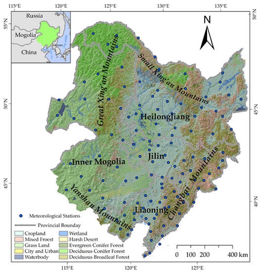
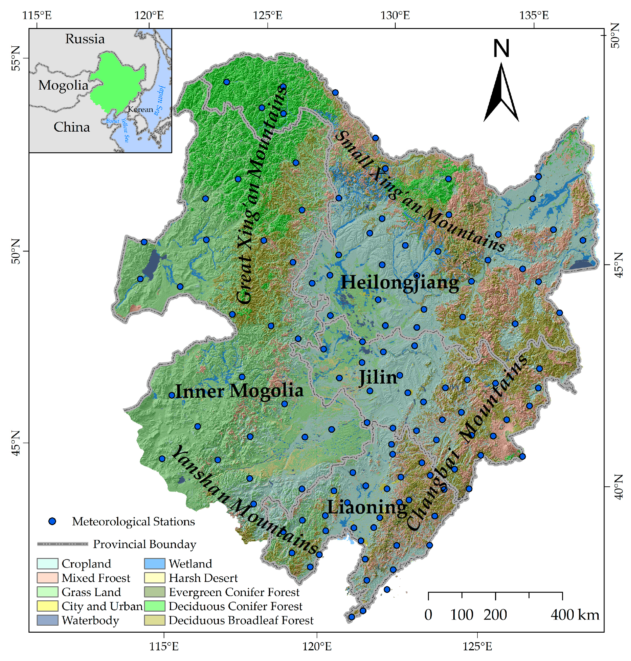
2.1. Study Area
2.2. Data
2.2.1. MODIS Data
2.2.2. Vegetation Index
2.2.3. Meteorological Data
2.2.4. Auxiliary Data
2.3. Methodology
2.3.1. Predictor Selection and Model Building
2.3.2. Model Calibration and Validation
3. Results
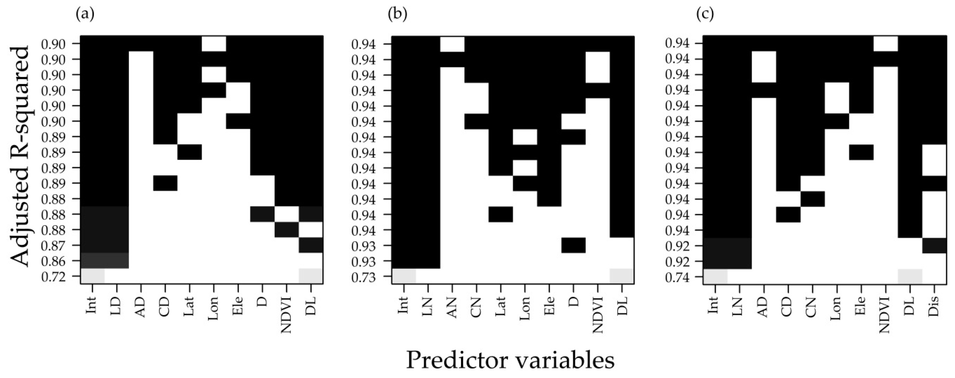
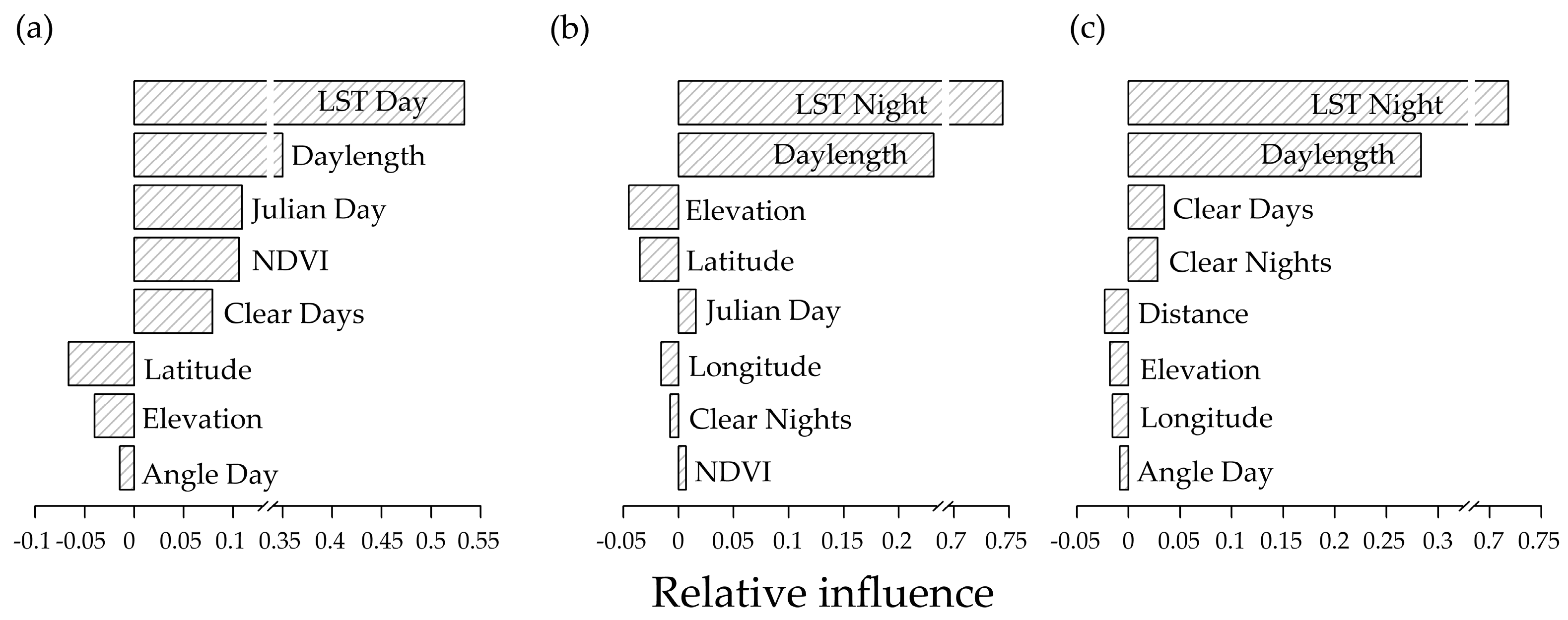
3.1. Variable and Model Selection
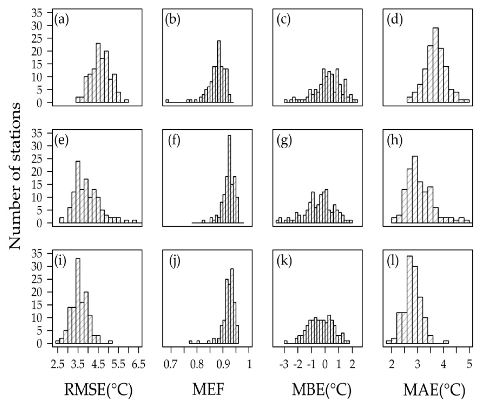
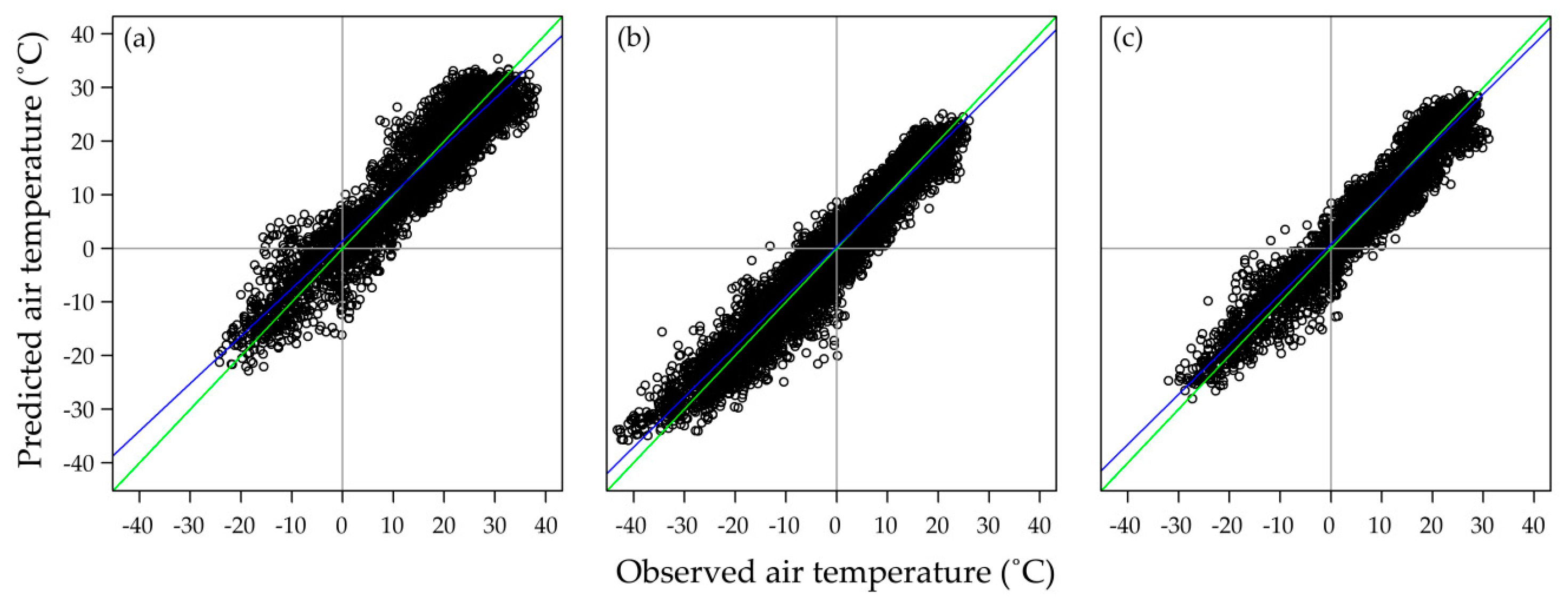
3.2. Model Validation
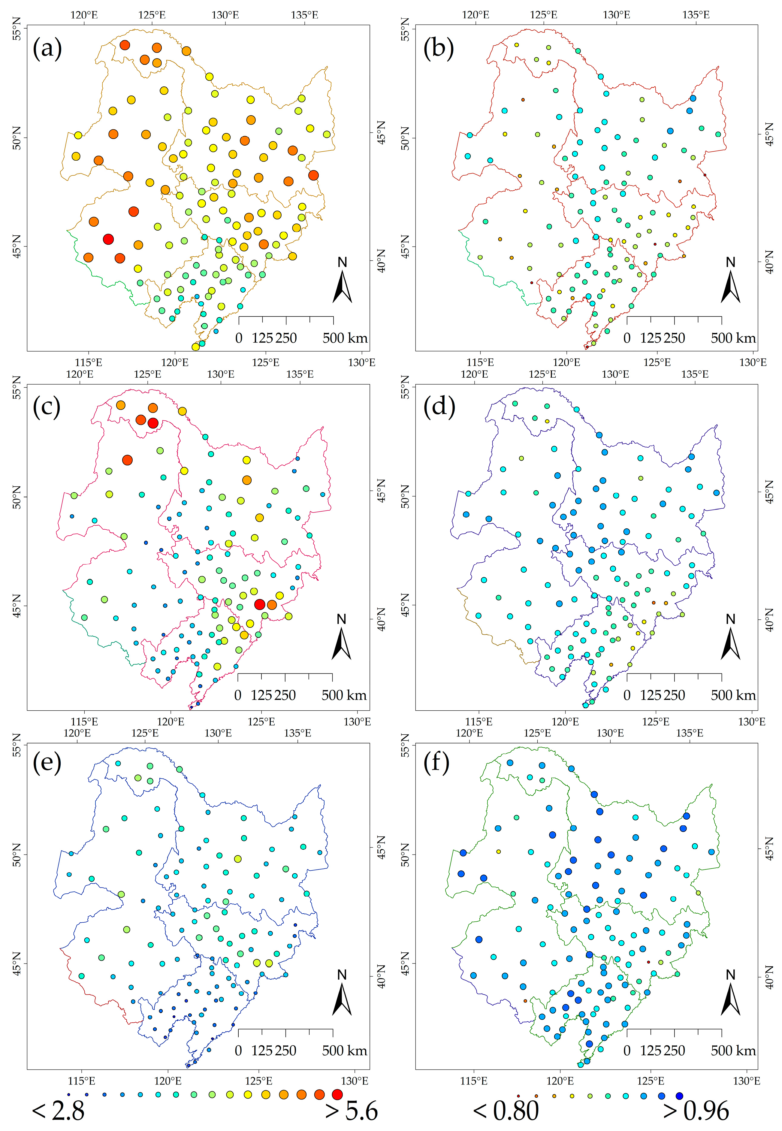
3.3. Spatial and Temporal Performance
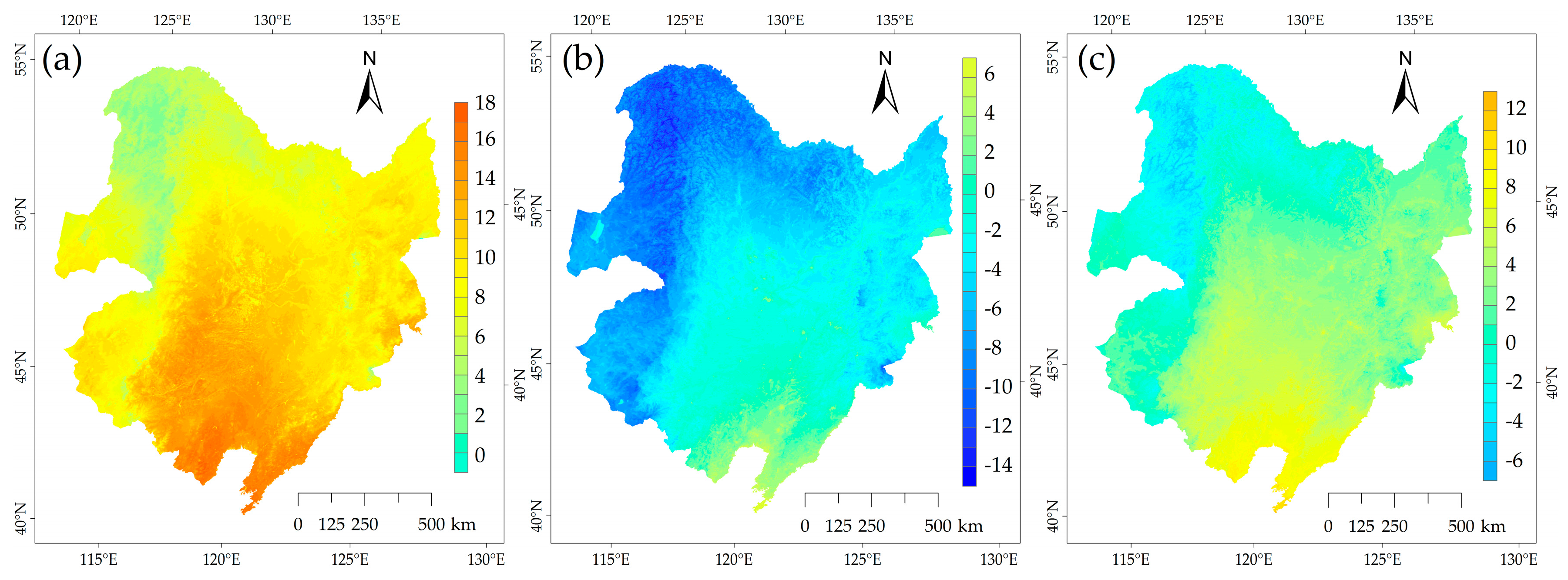
3.4. Patterns of Estimated Annual Air Temperature
4. Discussion
4.1. Spatial Uncertainties of Models
4.2. Temporal Uncertainties of Models
4.3. Spatial Variations of Annual Air Temperature
5. Conclusions
Acknowledgments
Author Contributions
Conflicts of Interest
References
- Peón, J.; Carmen, R.; Javier, F.C. Improvements in the Estimation of Daily Minimum Air Temperature in Peninsular Spain Using MODIS Land Surface Temperature. Int. J. Remote Sens. 2014, 35, 5148–5166. [Google Scholar] [CrossRef]
- Prihodko, L.; Goward, S.N. Estimation of Air Temperature from Remotely Sensed Surface Observations. Remote Sens. Environ. 1997, 60, 335–346. [Google Scholar] [CrossRef]
- Stisen, S.; Sandholt, I.; Nørgaard, A.; Fensholt, R.; Eklundh, L. Estimation of Diurnal Air Temperature Using Msg Seviri Data in West Africa. Remote Sens. Environ. 2007, 110, 262–274. [Google Scholar] [CrossRef]
- Shamir, E.; Georgakakos, K.P. MODIS Land Surface Temperature as an Index of Surface Air Temperature for Operational Snowpack Estimation. Remote Sens. Environ. 2014, 152, 83–98. [Google Scholar] [CrossRef]
- Benali, A.; Carvalho, A.C.; Nunes, J.P.; Carvalhais, N.; Santos, A. Estimating Air Surface Temperature in Portugal Using MODIS Lst Data. Remote Sens. Environ. 2012, 124, 108–121. [Google Scholar] [CrossRef]
- Westerling, A.L.; Hidalgo, H.G.; Cayan, D.R.; Swetnam, T.W. Warming and Earlier Spring Increase Western U.S. Forest Wildfire Activity. Science 2006, 313, 940–943. [Google Scholar] [CrossRef] [PubMed]
- Chen, Y.; Randerson, J.T.; Morton, D.C.; DeFries, R.S.; Collatz, G.J.; Kasibhatla, P.S.; Giglio, L.; Jin, Y.; Marlier, M.E. Forecasting Fire Season Severity in South America Using Sea Surface Temperature Anomalies. Science 2011, 334, 787–791. [Google Scholar] [CrossRef] [PubMed]
- Manzo-Delgado, L.; Sánchez-Colón, S.; Álvarez, R. Assessment of Seasonal Forest Fire Risk Using Noaa-Avhrr: A Case Study in Central Mexico. Int. J. Remote Sens. 2009, 30, 4991–5013. [Google Scholar] [CrossRef]
- Reich, P.B.; Luo, Y.; Bradford, J.B.; Poorter, H.; Perry, C.H.; Oleksyn, J. Temperature Drives Global Patterns in Forest Biomass Distribution in Leaves, Stems, and Roots. Proc. Natl. Acad. Sci. USA 2014, 111, 13721–13726. [Google Scholar] [CrossRef] [PubMed]
- Ruane, A.C.; McDermid, S.; Rosenzweig, C.; Baigorria, G.A.; Jones, J.W.; Romero, C.C.; Cecil, L.D. Carbon-Temperature-Water Change Analysis for Peanut Production under Climate Change: A Prototype for the Agmip Coordinated Climate-Crop Modeling Project (C3mp). Glob. Chang. Biol. 2014, 20, 394–407. [Google Scholar] [CrossRef] [PubMed]
- Rosenzweig, C.; Elliott, J.; Deryng, D.; Ruane, A.C.; Muller, C.; Arneth, A.; Boote, K.J.; Folberth, C.; Glotter, M.; Khabarov, N.; et al. Assessing Agricultural Risks of Climate Change in the 21st Century in a Global Gridded Crop Model Intercomparison. Proc. Natl. Acad. Sci. USA 2014, 111, 3268–3273. [Google Scholar] [CrossRef] [PubMed]
- Oyler, J.W.; Ballantyne, A.; Jencso, K.; Sweet, M.; Running, S.W. Creating a Topoclimatic Daily Air Temperature Dataset for the Conterminous United States Using Homogenized Station Data and Remotely Sensed Land Skin Temperature. Int. J. Climatol. 2015, 35, 2258–2279. [Google Scholar] [CrossRef]
- Beier, C.M.; Signell, S.A.; Luttman, A.; DeGaetano, A.T. High-Resolution Climate Change Mapping with Gridded Historical Climate Products. Landsc. Ecol. 2012, 27, 327–342. [Google Scholar] [CrossRef]
- Urban, M.; Eberle, J.; Hüttich, C.; Schmullius, C.; Herold, M. Comparison of Satellite-Derived Land Surface Temperature and Air Temperature from Meteorological Stations on the Pan-Arctic Scale. Remote Sens. 2013, 5, 2348–2367. [Google Scholar] [CrossRef]
- Vancutsem, C.; Ceccato, P.; Dinku, T.; Connor, S.J. Evaluation of MODIS Land Surface Temperature Data to Estimate Air Temperature in Different Ecosystems over Africa. Remote Sens. Environ. 2010, 114, 449–465. [Google Scholar] [CrossRef]
- Zhu, W.; Lű, A.; Jia, S. Estimation of Daily Maximum and Minimum Air Temperature Using MODIS Land Surface Temperature Products. Remote Sens. Environ. 2013, 130, 62–73. [Google Scholar] [CrossRef]
- Kloog, I.; Nordio, F.; Coull, B.A.; Schwartz, J. Predicting Spatiotemporal Mean Air Temperature Using MODIS Satellite Surface Temperature Measurements across the Northeastern USA. Remote Sens. Environ. 2014, 150, 132–139. [Google Scholar] [CrossRef]
- Williamson, S.N.; Hik, D.S.; Gamon, J.A.; Kavanaugh, J.L.; Flowers, G.E. Estimating Temperature Fields from MODIS Land Surface Temperature and Air Temperature Observations in a Sub-Arctic Alpine Environment. Remote Sens. 2014, 6, 946–963. [Google Scholar] [CrossRef]
- Vincent, L.A.; Mekis, E. Changes in Daily and Extreme Temperature and Precipitation Indices for Canada over the Twentieth Century. Atmos. Ocean 2006, 44, 177–193. [Google Scholar] [CrossRef]
- Carlson, T. An Overview of the “Triangle Method” for Estimating Surface Evapotranspiration and Soil Moisture from Satellite Imagery. Sensors 2007, 7, 1612–1629. [Google Scholar] [CrossRef]
- Zhang, W.; Huang, Y.; Yu, Y.; Sun, W. Empirical Models for Estimating Daily Maximum, Minimum and Mean Air Temperatures with MODIS Land Surface Temperatures. Int. J. Remote Sens. 2011, 32, 9415–9440. [Google Scholar] [CrossRef]
- Lin, X.; Zhang, W.; Huang, Y.; Sun, W.; Han, P.; Yu, L.; Sun, F. Empirical Estimation of near-Surface Air Temperature in China from MODIS Lst Data by Considering Physiographic Features. Remote Sens. 2016, 8. [Google Scholar] [CrossRef]
- Hanna, M.; Katurji, M.; Appelhans, T.; Müller, M.U.; Nauss, T.; Roudier, P.; Zawar-Reza, P. Mapping Daily Air Temperature for Antarctica Based on MODIS LST. Remote Sens. 2016, 8. [Google Scholar] [CrossRef]
- Zhang, H.B.; Zhang, F.; Ye, M.; Che, T.; Zhang, G.Q. Estimating Daily Air Temperatures over the Tibetan Plateau by Dynamically Integrating MODIS Lst Data. J. Geophys. Res. Atmos. 2016, 121, 11425–11441. [Google Scholar] [CrossRef]
- Tao, J.; Zhang, Y.; Zhu, J.; Jiang, Y.; Zhang, X.; Zhang, T.; Xi, Y. Elevation-Dependent Temperature Change in the Qinghai–Xizang Plateau Grassland During the Past Decade. Theor. Appl. Climatol. 2013, 117, 61–71. [Google Scholar] [CrossRef]
- Nieto, H.; Sandholt, I.; Aguado, I.; Chuvieco, E.; Stisen, S. Air Temperature Estimation with Msg-Seviri Data: Calibration and Validation of the TVX Algorithm for the Iberian Peninsula. Remote Sens. Environ. 2011, 115, 107–116. [Google Scholar] [CrossRef]
- Fang, J.; Chen, A.; Peng, C.; Zhao, S.; Ci, L. Changes in Forest Biomass Carbon Storage in China between 1949 and 1998. Science 2001, 292, 2320–2322. [Google Scholar] [CrossRef] [PubMed]
- Piao, S.; Fang, J.; Ciais, P.; Peylin, P.; Huang, Y.; Sitch, S.; Wang, T. The Carbon Balance of Terrestrial Ecosystems in China. Nature 2009, 458, 1009–1013. [Google Scholar] [CrossRef] [PubMed]
- Liu, Z.; Yang, J.; Chang, Y.; Weisberg, P.J.; He, H.S. Spatial Patterns and Drivers of Fire Occurrence and Its Future Trend under Climate Change in a Boreal Forest of Northeast China. Glob. Chang. Biol. 2012, 18, 2041–2056. [Google Scholar] [CrossRef]
- Cai, W.; Yang, J.; Liu, Z.; Hu, Y.; Weisberg, P.J. Post-Fire Tree Recruitment of a Boreal Larch Forest in Northeast China. For. Ecol. Manag. 2013, 307, 20–29. [Google Scholar] [CrossRef]
- Welch, J.R.; Vincent, J.R.; Auffhammer, M.; Moya, P.F.; Dobermann, A.; Dawe, D. Rice Yields in Tropical/Subtropical Asia Exhibit Large but Opposing Sensitivities to Minimum and Maximum Temperatures. Proc. Natl. Acad. Sci. USA 2010, 107, 14562–14567. [Google Scholar] [CrossRef] [PubMed]
- van Wart, J.; Grassini, P.; Cassman, K.G. Impact of Derived Global Weather Data on Simulated Crop Yields. Glob. Chang. Biol. 2013, 19, 3822–3834. [Google Scholar] [CrossRef] [PubMed]
- Mildrexler, D.J.; Zhao, M.; Running, S.W. A Global Comparison between Station Air Temperatures and MODIS Land Surface Temperatures Reveals the Cooling Role of Forests. J. Geophys. Res. 2011, 116. [Google Scholar] [CrossRef]
- Zhang, P.; Bounoua, L.; Imhoff, M.L.; Wolfe, R.E.; Thome, K. Comparison of MODIS Land Surface Temperature and Air Temperature over the Continental USA Meteorological Stations. Can. J. Remote Sens. 2014, 40, 110–122. [Google Scholar]
- Wan, Z.; Zhang, Y.; Zhang, Q.; Li, Z.L. Validation of the Land-Surface Temperature Products Retrieved from Terra Moderate Resolution Imaging Spectroradiometer Data. Remote Sens. Environ. 2002, 83, 163–180. [Google Scholar] [CrossRef]
- MODIS Land Surface Temperature Products User’s Guide. Available online: http://www.icess.ucsb.edu/MODIS/LstUsrGuide/usrguide.html (accessed on December 2013).
- Stow, D.A.; Hope, A.; McGuire, D.; Verbyla, D.; Gamon, J.; Huemmrich, F.; Houston, S.; Racine, C.; Sturm, M.; Tape, K.; et al. Remote Sensing of Vegetation and Land-Cover Change in Arctic Tundra Ecosystems. Remote Sens. Environ. 2004, 89, 281–308. [Google Scholar] [CrossRef]
- Raynolds, M.; Comiso, J.; Walker, D.; Verbyla, D. Relationship between Satellite-Derived Land Surface Temperatures, Arctic Vegetation Types, and NDVI. Remote Sens. Environ. 2008, 112, 1884–1894. [Google Scholar] [CrossRef]
- Bustos, E.; Meza, F.J. A Method to Estimate Maximum and Minimum Air Temperature Using MODIS Surface Temperature and Vegetation Data: Application to the Maipo Basin, Chile. Theor. Appl. Climatol. 2014. [Google Scholar] [CrossRef]
- Raynolds, M.K.; Walker, D.A.; Maier, H.A. NDVI Patterns and Phytomass Distribution in the Circumpolar Arctic. Remote Sens. Environ. 2006, 102, 271–281. [Google Scholar] [CrossRef]
- Zheng, X.; Zhu, J.; Yan, Q. Monthly Air Temperatures over Northern China Estimated by Integrating MODIS Data with Gis Techniques. J. Appl. Meteorol. Climatol. 2013, 52, 1987–2000. [Google Scholar] [CrossRef]
- Neitsch, S.L.; Arnold, J.G.; Kiniry, J.R.; Williams, J.R.; King, K.W. Soil and Water Assessment Tool: Theoretical Documentation; Version 2009; Texas Water Resources Institute: College Station, TX, USA, 2011; pp. 30–32. [Google Scholar]
- Neteler, M. Estimating Daily Land Surface Temperature in Mountainous Environments by Reconstructed MODIS LST Data. Remote Sens. 2010, 2, 333–351. [Google Scholar] [CrossRef]
- Ke, L.H.; Wang, Z.X.; Song, C.Q.; Lu, Z.Q. Reconstruction of MODIS Land Surface Temperature in Northeast Qinghai-Xizang Plateau and LST Comparison with Air Temperature. Plateau Meteorol. 2011, 30, 277–287. [Google Scholar]
- Zurr, A.F.; Ieno, E.N.; Elphick, C.S. A Protocol for Data Exploration to Avoid Common Statistical Problems. Methods Ecol. Evol. 2010, 1, 3–14. [Google Scholar] [CrossRef]
- Dormann, C.F.; Elith, J.; Bacher, S.; Buchmann, C.; Carl, G.; Carré, G.; Marquéz, J.R.G.; Gruber, B.; Lafourcade, B.; Leitão, P.J. Collinearity: A review of methods to deal with it and a simulation study evaluating their performance. Ecography 2013, 36, 027–046. [Google Scholar] [CrossRef]
- Willmott, C.J.; Matsuura, K. Advantages of the Mean Absolute Error (Mae) over the Root Mean Square Error (Rmse) in Assessing Average Model Performance. Clim. Res. 2005, 30, 79–82. [Google Scholar] [CrossRef]
- Dobrowski, S.Z.; Abatzoglou, J.T.; Greenberg, J.A.; Schladow, S.G. How Much Influence Does Landscape-Scale Physiography Have on Air Temperature in a Mountain Environment? Agric. For. Meteorol. 2009, 149, 1751–1758. [Google Scholar] [CrossRef]
- Van De Kerchove, R.; Lhermitte, S.; Veraverbeke, S.; Goossens, R. Spatio-Temporal Variability in Remotely Sensed Land Surface Temperature, and Its Relationship with Physiographic Variables in the Russian Altay Mountains. Int. J. Appl. Earth Obs. Geoinf. 2013, 20, 4–19. [Google Scholar] [CrossRef]
- Yan, H.; Zhang, J.; Hou, Y.; He, Y. Estimation of Air Temperature from MODIS Data in East China. Int. J. Remote Sens. 2009, 30, 6261–6275. [Google Scholar] [CrossRef]
- Zeng, L.; Wardlow, B.D.; Tadesse, T.; Shan, J.; Hayes, M.; Li, D.; Xiang, D. Estimation of Daily Air Temperature Based on MODIS Land Surface Temperature Products over the Corn Belt in the US. Remote Sens. 2015, 7, 951–970. [Google Scholar] [CrossRef]
- Kaufmann, R.K.; Zhou, L.; Myneni, R.B.; Tucker, C.J.; Slayback, D.; Shabanov, N.V.; Pinzon, J. The Effect of Vegetation on Surface Temperature: A Statistical Analysis of NDVI and Climate Data. Geophys. Res. Let. 2003, 30. [Google Scholar] [CrossRef]
- Jeong, S.J.; Ho, C.H.; Jeong, J.H. Increase in Vegetation Greenness and Decrease in Springtime Warming over East Asia. Geophys. Res. Lett. 2009, 36. [Google Scholar] [CrossRef]
- Pouteau, R.; Rambal, S.; Ratte, J.P.; Gogé, F.; Joffre, R.; Winkel, T. Downscaling MODIS-Derived Maps Using Gis and Boosted Regression Trees: The Case of Frost Occurrence over the Arid Andean Highlands of Bolivia. Remote Sens. Environ. 2011, 115, 117–129. [Google Scholar] [CrossRef]
- Shen, S.; Leptoukh, G.G. Estimation of Surface Air Temperature over Central and Eastern Eurasia from MODIS Land Surface Temperature. Environ. Res. Lett. 2011, 6. [Google Scholar] [CrossRef]
- Tian, Z.; Jiang, D. Revisiting Last Glacial Maximum Climate over China and East Asian Monsoon Using Pmip3 Simulations. Palaeogeogr. Palaeoclimatol. Palaeoecol. 2016, 453, 115–126. [Google Scholar] [CrossRef]
- Sun, L.; Shen, B.; Sui, B.; Huang, B. The Influences of East Asian Monsoon on Summer Precipitation in Northeast China. Clim. Dyn. 2016. [Google Scholar] [CrossRef]
- Mostovoy, G.V.; King, R.L.; Reddy, K.R.; Kakani, V.G.; Filippova, M.G. Statistical Estimation of Daily Maximum and Minimum Air Temperatures from MODIS Lst Data over the State of Mississippi. Gisci. Remote Sens. 2006, 43, 78–110. [Google Scholar] [CrossRef]
- Huang, R.; Zhang, C.; Huang, J.; Zhu, D.; Wang, L.; Liu, J. Mapping of Daily Mean Air Temperature in Agricultural Regions Using Daytime and Nighttime Land Surface Temperatures Derived from Terra and Aqua MODIS Data. Remote Sens. 2015, 7, 8728–8756. [Google Scholar] [CrossRef]


| Abbreviation | Variable | Source | Explanation |
|---|---|---|---|
| LD, LN | Land Surface Temperature | MODIS | 8-day average Land Surface temperature layers derived over the 2002–2016 time period using MYD11A2 product |
| AD, AN | View Zenith Angle | ||
| TD, TN | View Time | ||
| CD, CN | Clear Days | ||
| NDVI | Normalized difference vegetation index | MODIS | Calculated Normalized Difference Vegetation Index using 8-day average the surface spectral reflectance layers derived over the 2002–2016 time period using MYD09A1 product |
| D | Julian day | Meteorological data | The continuous count of days was from 1 January to the last day every year |
| DL | Day length | Meteorological data | Calculated the 8-day average day length using Julian day and latitude in the meteorological data |
| Lon | Longitude | Meteorological data | The geographical location of meteorological stations was extracted from meteorological metadata |
| Lat | Latitude | ||
| Ele | Elevation | DEM | The altitude extracted from a 90 m resolution digital elevation model (DEM) according to the location of meteorological stations |
| Dis | Distance to the coast | GSHHS coastline | Distance to the coast was calculated based on the GSHHS coastline in the ESRI ArcGIS 9.3 |
| Tmax, Tmin, Tmean | Maximum, Minimum and Average Temperature | Meteorological data | Calculated the 8-day average day maximum, minimum and average temperature according to meteorological data |
| Model Equations | Adj R2 | RMSE | MFE | CRM | MBE | MAE | 2.5% | 97.5% | |
|---|---|---|---|---|---|---|---|---|---|
| (1) | Max = 0.8158 × LD − 0.8104 | 0.86 | 5.21 | 0.86 | 0.02 | 0.30 | 4.15 | −10.94 | 9.49 |
| (2) | Max = 0.5899 LD + 0.5421 CD + 1.1267 DL + 9.880 NDVI − 15.2347 | 0.89 | 4.75 | 0.88 | 0.02 | 0.24 | 3.79 | −9.52 | 9.14 |
| (3) | Max = 0.5560 LD + 0.0130 D + 1.5538 DL + 8.2394 NDVI − 20.0725 | 0.89 | 4.77 | 0.88 | 0.02 | 0.22 | 3.80 | −10.01 | 8.76 |
| (4) | Max = 0.5082 LD − 0.2578 Lat + 0.0152 D + 1.9 DL + 7.631 NDVI − 12.23 | 0.89 | 4.75 | 0.88 | 0.01 | 0.20 | 3.77 | −9.77 | 8.86 |
| (5) | Max = 0.5350 LD + 0.5312 CD + 0.0128 D + 1.6670 DL + 7.7470 NDVI − 22.6600 | 0.89 | 4.68 | 0.89 | 0.02 | 0.22 | 3.73 | −9.57 | 8.83 |
| (6) | Max = 0.519 LD + 0.5729 CD − 0.0033 Ele + 0.0134 D + 1.778 DL + 7.711 NDVI − 23.03 | 0.90 | 4.64 | 0.89 | 0.02 | 0.21 | 3.69 | −9.36 | 8.83 |
| (7) | Max = 0.4726 LD + 0.6268 CD − 0.3161 Lat + 0.0155 D + 2.112 DL + 6.913 NDVI − 13.51 | 0.90 | 4.63 | 0.89 | 0.01 | 0.19 | 3.69 | −9.24 | 8.89 |
| (8) | Min = 0.9714 LN + 1.6738 | 0.93 | 4.20 | 0.92 | 0.43 | −0.48 | 3.22 | −8.63 | 8.06 |
| (9) | Min = 0.8262 LN + 1.0985 DL − 11.8179 | 0.94 | 4.04 | 0.93 | 0.39 | −0.44 | 3.12 | −8.21 | 7.91 |
| (10) | Min = 0.7933 LN − 0.1857 Lat + 1.2719 DL − 5.6884 | 0.94 | 4.00 | 0.93 | 0.38 | −0.43 | 3.10 | −8.05 | 7.88 |
| (11) | Min = 0.8053 LN − 0.0026 Ele + 1.209 DL − 12.42 | 0.94 | 3.99 | 0.93 | 0.38 | −0.43 | 3.09 | −8.04 | 7.84 |
| (12) | Mean = 0.9466 LN + 7.3698 | 0.92 | 4.09 | 0.91 | −0.05 | −0.36 | 3.12 | −8.28 | 8.04 |
| (13) | Mean = 0.7479 LN + 1.5114 DL − 11.2209 | 0.94 | 3.67 | 0.93 | −0.04 | −0.31 | 2.86 | −7.25 | 7.21 |
| (14) | Mean = 0.7343 LN + 1.5545 DL + 0.3246 CD − 12.8276 | 0.94 | 3.63 | 0.93 | −0.04 | −0.30 | 2.82 | −7.23 | 7.16 |
| (15) | Mean = 0.7513 LN + 1.5653 DL + 0.3240 CN − 13.2565 | 0.94 | 3.60 | 0.93 | −0.04 | −0.29 | 2.80 | −7.21 | 7.02 |
| Land Cover | Tmax | Tmin | Tmean | ||||||||||||
|---|---|---|---|---|---|---|---|---|---|---|---|---|---|---|---|
| RMSE | MFE | CRM | MBE | MAE | RMSE | MFE | CRM | MBE | MAE | RMSE | MFE | CRM | MBE | MAE | |
| Urban | 4.62 | 0.89 | 0.03 | 0.44 | 3.71 | 3.97 | 0.93 | 0.75 | –0.65 | 3.09 | 3.63 | 0.93 | −0.09 | −0.68 | 2.84 |
| Farmland | 4.55 | 0.89 | 0.02 | 0.27 | 3.61 | 3.82 | 0.93 | −0.23 | 0.08 | 2.96 | 3.53 | 0.93 | 0.03 | 0.22 | 2.72 |
| Forest | 4.77 | 0.84 | −0.04 | −0.57 | 3.73 | 4.81 | 0.90 | 0.34 | −0.92 | 3.61 | 3.76 | 0.90 | −0.12 | −1.01 | 2.88 |
| Grass | 5.09 | 0.88 | −0.06 | −0.67 | 4.06 | 4.33 | 0.92 | 0.11 | −0.54 | 3.41 | 3.77 | 0.93 | −0.09 | −0.43 | 2.99 |
| Seasons | Tmax | Tmin | Tmean | ||||||||||||
|---|---|---|---|---|---|---|---|---|---|---|---|---|---|---|---|
| RMSE | MFE | CRM | MBE | MAE | RMSE | MFE | CRM | MBE | MAE | RMSE | MFE | CRM | MBE | MAE | |
| Spring | 4.80 | 0.75 | 0.01 | 0.09 | 3.85 | 3.64 | 0.85 | −0.30 | −0.55 | 2.91 | 3.67 | 0.83 | 0.02 | 0.21 | 2.92 |
| Summer | 3.82 | −0.04 | 0.01 | 0.20 | 3.06 | 2.71 | 0.62 | −0.04 | −0.69 | 2.11 | 2.70 | 0.45 | −0.05 | −1.06 | 2.13 |
| Autumn | 4.96 | 0.78 | 0.05 | 0.58 | 4.00 | 4.15 | 0.82 | 0.11 | −0.21 | 3.34 | 3.66 | 0.85 | 0.04 | 0.22 | 2.91 |
| Winter | 5.10 | 0.57 | 0.04 | −0.25 | 4.04 | 5.02 | 0.66 | 0.01 | −0.27 | 3.93 | 4.51 | 0.68 | 0.05 | −0.61 | 3.51 |
| Month | Tmax | Tmin | Tmean | ||||||||||||
|---|---|---|---|---|---|---|---|---|---|---|---|---|---|---|---|
| RMSE | MFE | CRM | MBE | MAE | RMSE | MFE | CRM | MBE | MAE | RMSE | MFE | CRM | MBE | MAE | |
| January | 5.23 | 0.53 | −0.15 | 1.40 | 4.04 | 4.52 | 0.72 | 0.01 | −0.21 | 3.55 | 4.21 | 0.69 | 0.07 | −1.05 | 3.36 |
| February | 4.76 | 0.56 | −0.06 | 0.21 | 3.86 | 5.47 | 0.62 | 0.05 | −0.77 | 4.43 | 4.34 | 0.68 | 0.05 | −0.55 | 3.50 |
| March | 4.81 | 0.57 | −0.05 | −0.35 | 3.84 | 3.78 | 0.71 | 0.18 | −1.16 | 3.01 | 3.59 | 0.68 | −3.22 | −1.01 | 2.87 |
| April | 4.60 | 0.50 | 0.07 | 1.36 | 3.84 | 3.42 | 0.62 | −0.10 | −0.27 | 2.73 | 3.69 | 0.54 | 0.15 | 1.60 | 2.94 |
| May | 4.95 | 0.34 | −0.03 | −0.61 | 3.88 | 3.68 | 0.61 | −0.01 | −0.14 | 2.95 | 3.72 | 0.54 | 0.01 | 0.16 | 2.94 |
| June | 4.13 | −0.28 | −0.08 | −2.00 | 3.25 | 2.64 | 0.55 | −0.07 | −1.01 | 2.01 | 3.16 | 0.10 | −0.10 | −1.97 | 2.52 |
| July | 3.48 | −0.15 | 0.03 | 0.87 | 2.79 | 2.69 | 0.44 | −0.02 | −0.35 | 2.11 | 2.51 | 0.26 | −0.03 | −0.80 | 1.97 |
| August | 3.81 | 0.07 | 0.07 | 1.70 | 3.11 | 2.80 | 0.62 | −0.05 | −0.67 | 2.22 | 2.36 | 0.57 | −0.02 | −0.38 | 1.87 |
| September | 4.46 | 0.30 | 0.09 | 1.80 | 3.58 | 3.72 | 0.56 | −0.03 | −0.21 | 3.06 | 3.25 | 0.59 | 0.06 | 0.81 | 2.62 |
| October | 5.05 | 0.36 | 0.12 | 1.31 | 4.18 | 4.11 | 0.53 | 0.12 | −0.24 | 3.34 | 3.59 | 0.58 | 0.12 | 0.50 | 2.90 |
| November | 5.48 | 0.36 | −23.03 | −1.68 | 4.38 | 4.60 | 0.64 | 0.02 | −0.19 | 3.64 | 4.23 | 0.62 | 0.16 | −0.86 | 3.33 |
| December | 5.32 | 0.47 | 0.29 | −2.21 | 4.23 | 5.02 | 0.60 | −0.01 | 0.20 | 3.81 | 4.92 | 0.58 | 0.02 | −0.28 | 3.66 |
© 2017 by the authors. Licensee MDPI, Basel, Switzerland. This article is an open access article distributed under the terms and conditions of the Creative Commons Attribution (CC BY) license (http://creativecommons.org/licenses/by/4.0/).
Share and Cite
Yang, Y.Z.; Cai, W.H.; Yang, J. Evaluation of MODIS Land Surface Temperature Data to Estimate Near-Surface Air Temperature in Northeast China. Remote Sens. 2017, 9, 410. https://doi.org/10.3390/rs9050410
Yang YZ, Cai WH, Yang J. Evaluation of MODIS Land Surface Temperature Data to Estimate Near-Surface Air Temperature in Northeast China. Remote Sensing. 2017; 9(5):410. https://doi.org/10.3390/rs9050410
Chicago/Turabian StyleYang, Yuan Z., Wen H. Cai, and Jian Yang. 2017. "Evaluation of MODIS Land Surface Temperature Data to Estimate Near-Surface Air Temperature in Northeast China" Remote Sensing 9, no. 5: 410. https://doi.org/10.3390/rs9050410
APA StyleYang, Y. Z., Cai, W. H., & Yang, J. (2017). Evaluation of MODIS Land Surface Temperature Data to Estimate Near-Surface Air Temperature in Northeast China. Remote Sensing, 9(5), 410. https://doi.org/10.3390/rs9050410