A Novel Pan-Sharpening Framework Based on Matting Model and Multiscale Transform

Abstract

Pan-sharpening aims to sharpen a low spatial resolution multispectral (MS) image by combining the spatial detail information extracted from a panchromatic (PAN) image. An effective pan-sharpening method should produce a high spatial resolution MS image while preserving more spectral information. Unlike traditional intensity-hue-saturation (IHS)- and principal component analysis (PCA)-based multiscale transform methods, a novel pan-sharpening framework based on the matting model (MM) and multiscale transform is presented in this paper. First, we use the intensity component (I) of the MS image as the alpha channel to generate the spectral foreground and background. Then, an appropriate multiscale transform is utilized to fuse the PAN image and the upsampled I component to obtain the fused high-resolution gray image. In the fusion, two preeminent fusion rules are proposed to fuse the low- and high-frequency coefficients in the transform domain. Finally, the high-resolution sharpened MS image is obtained by linearly compositing the fused gray image with the upsampled foreground and background images. The proposed framework is the first work in the pan-sharpening field. A large number of experiments were tested on various satellite datasets; the subjective visual and objective evaluation results indicate that the proposed method performs better than the IHS- and PCA-based frameworks, as well as other state-of-the-art pan-sharpening methods both in terms of spatial quality and spectral maintenance.

1. Introduction

High-resolution multichannel satellite images with both high spatial resolution and spectral diversity are required in many image-processing applications, such as change detection, land-cover segmentation, and road extraction. However, due to the limits on the signal-to-noise ratio, these acquisitive images cannot be achieved only through a single sensor [1]. Thus, most remote sensing satellites (e.g., WorldView-2, QuickBird, IKONOS) simultaneously provide a panchromatic (PAN) image with high spatial but low spectral resolution, and a multispectral (MS) image with complementary properties [2,3]. Then, a pan-sharpening algorithm is applied to merge the MS and PAN images to have a high spatial resolution MS image, preserving the spectral information of MS. When the spatial details are obtained from a multispectral/hyperspectral sequence, the pan- sharpening algorithm is called hyper-sharpening [4].

In the last two decades, many pan-sharpening methods have been proposed to fuse MS and PAN images. A detailed comparison of the characteristics and performance of classical and famous pan-sharpening methods was presented in [5]. Initial efforts mainly focus on the component substitution-based (CS) methods, such as the principal component analysis (PCA) method [6], the intensity-hue-saturation (IHS) method [7,8] and the Gram–Schmidt (GS) method [9]. The primary concept of these CS-based methods is to first transform the upsampled MS images to a new space. If one component of the new space contains equivalent structures to those of the PAN image, fusion occurs by totally or partially substituting this component with the PAN image. Finally, a corresponding inverse transform is performed to obtain the high-resolution pan-sharpened image. These CS-based methods are fast and easy to implement, but are not adaptable to the latest generation of high-resolution remote sensing images. A common problem that arises with these methods is the serious color change due to spectral distortion. The main reason for the spectral distortion is that the wavelength range of the new satellite PAN image is extended from the visible to the near infrared [10]. A possible simple modification of these schemes, also applicable to CS methods, replaces the interpolated MS image with its deblurred version, where the deblurring kernel is matched to the modulation transfer function (MTF) of the MS sensor [11]. Recently, pan-sharpening has also been formulated as a compressive sensing reconstruction problem, but this scheme has high computation complexity [12,13].

Multiresolution analysis (MRA)-based methods have attracted interest in the pan-sharpening field [14,15]. These include traditional pyramid-based methods such as Laplace transform (LP) [16] and gradient transform [17]; wavelet transform (WT)-based methods such as discrete wavelet transform (DWT) [18]; and dual-tree complex wavelet transform (DTCWT) [19], and burgeoning geometric analysis methods such as Curvelet transform [20], Contourlet transform [21] and Shearlet transform [22]. The MRA approaches extract high-pass spatial detail information from the PAN image and then inject them into each band of the MS image, interpolating at the same resolution as the high-resolution PAN image [23]. Compared to the CS methods, the MRA methods can preserve spectral characteristics in the sharpened image, but they usually suffer from spatial distortion problems, such as ringing or stair-casing phenomena [24].

To overcome the limits of MRA and CS methods, many researchers jointly adopted the CS and MRA methods to fuse the MS and PAN images [25]. These category methods are based on a CS frame. They fuse the representation component of the MS image and the PAN image by the use of various multiscale transforms. In addition, some predefined fusion rules are used in the fusion process. Then, the corresponding inverse transform is applied in the fused component and the other components of the MS image to obtain the final sharpened image. For example, Cheng et al. [26] jointly adopted IHS and WT to fuse IKONOS and QuickBird satellite images, in which WT was applied to the intensity component of the MS images and PAN image. The spectral information of the resultant images was improved through this method. Dong et al. [27] combined the IHS with the Curvelet transform to fuse remote sensing images, utilizing the better edge preservation property of Curvelet to enhance the spatial quality of the fused images. Shah et al. [28] proposed an adaptive PCA and Contourlet transform-based pan-sharpening method, in which the adaptive PCA was used to reduce the spectral distortion. Ourabia et al. [29] tried to find a compromise between the spatial resolution enhancement and the spectral information preservation at the same time by using enhanced PCA and nonsubsampled Contourlet transform (NSCT).

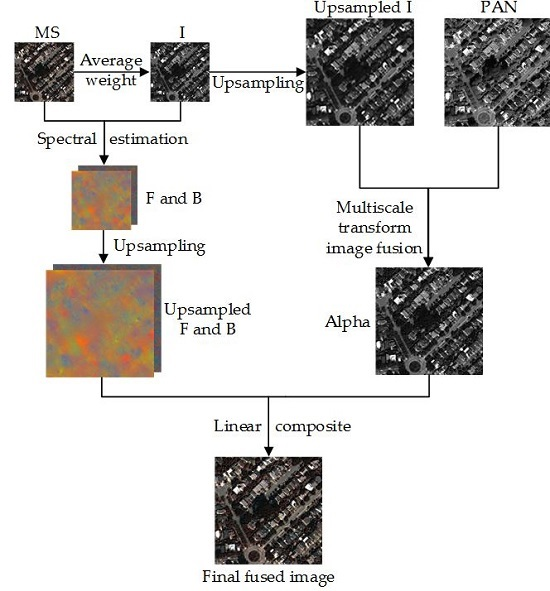
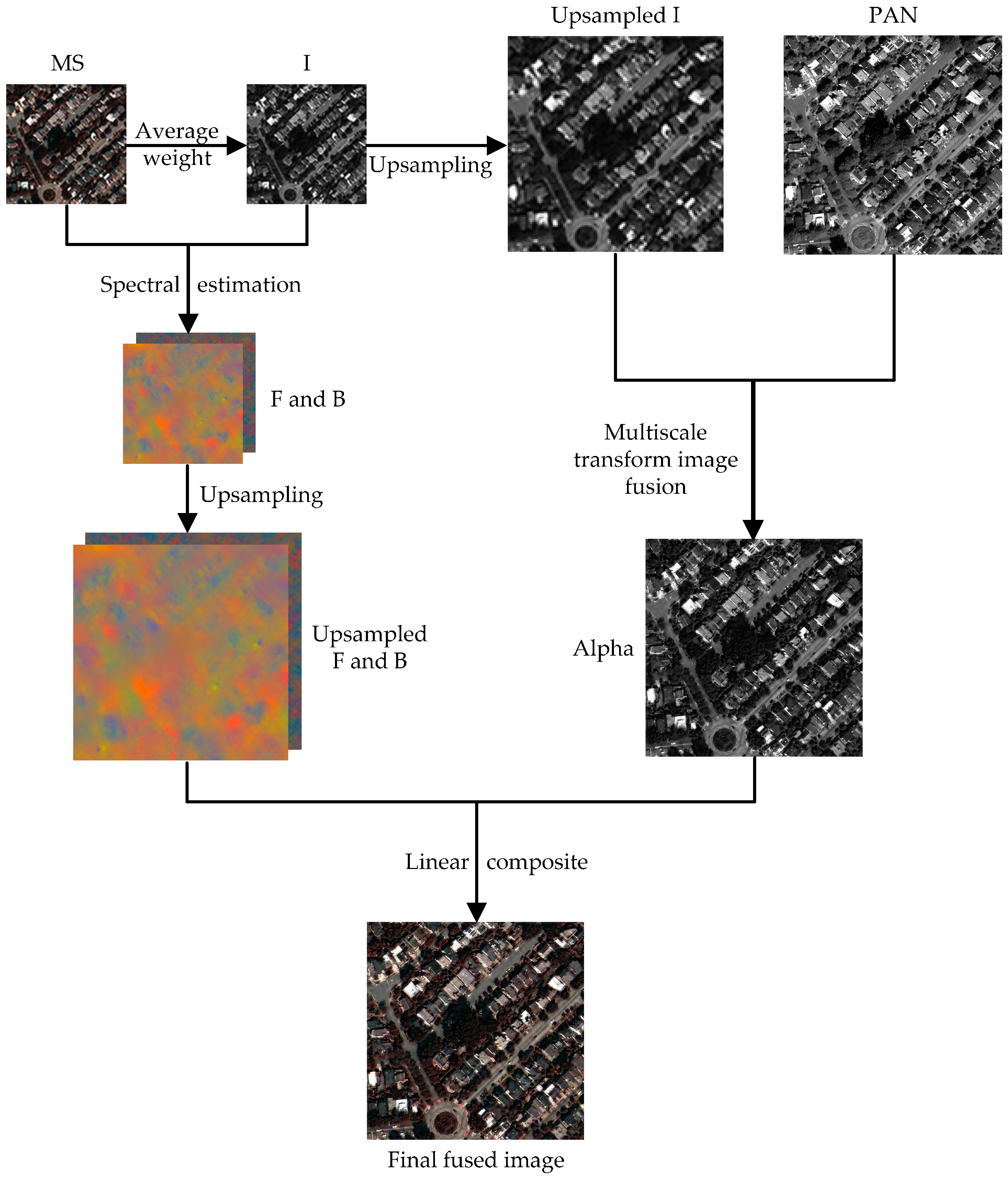
It can be seen that the foregoing hybrid methods improve performance to some extent, compared to the previous CS- or MRA-based pan-sharpening methods, but there are also some drawbacks to these frames. For example, the IHS transform-based frameworks are only feasible for three bands images, and the PCA transform-based frameworks result in serious spectral distortion. To improve the pan-sharpening performance, a novel pan-sharpening framework that is based on the matting model and multiscale transform is proposed in this paper. First, the I component of the MS image is selected as the alpha channel to estimate the foreground and background images with a local linear assumption. Then, the upsampled I component and the PAN image are fused by adopting a discretionary multiscale transform tool. Finally, a high-resolution sharpened MS image can be achieved by a composition operation on the fused image with the upsampled foreground and background images. The proposed framework has no limits regarding the amount of MS image bands. Thus, it can be directly applied for three, four, and even eight bands of MS images.

Furthermore, in terms of the multiscale transform, due to limits on directional selectivity, the classical WT can be sensitive to point-wise singularities, but cannot capture other types of salient features, such as lines. Therefore, WT often causes artifacts and Gibbs effects in the final fused results. To better represent high-order singular features, researchers have put forward a number of more effective multiresolution geometric analysis tools, such as the aforementioned Curvelet transform and Contourlet transform. These transforms are anisotropic and have good directional selectivity, so they can accurately represent the image edge information in different scales and directions. However, because there are down-sampling operations in their decompositions, they lack shift-invariance, resulting in the fused result being affected by the noise or mis-registration of source images. To overcome this disadvantage, Cunha et al. [30] proposed the NSCT, which is an improved version of the Contourlet transform. However, the computational complexity of NSCT is high, and thus the fusion process consumes too much time.

In recent years, an excellent multiresolution analysis tool named nonsubsampled Shearlet transform (NSST) was put forward and has been applied extensively [31]. The NSST is not only shift invariant, but also multiscale, and it exhibits multidirectional expansion; it maps the standard shearing filters from a false polarization grid system into a Cartesian coordinate system directly during the multidirectional decomposition procedure. This mapping process can maintain well deserved multiscale analyses properties while drastically reducing computation complexity. Thus, as an example, we choose the NSST in this paper due to its superiority compared to other multiscale transforms. Certainly, it can be extended to any other multiscale transform approach in the proposed framework if necessary.

In the multiscale transform image fusion process, the coefficient fusion rules are crucial. For the low-frequency coefficients, a gradient domain-based adaptive weighted averaging rule is proposed. Furthermore, as to the high-frequency coefficients, the simple but effective spatial frequency (SF) fusion rule is designed. Experiments on WorldView-2, QuickBird, and IKONOS satellite images demonstrate that the proposed method outperforms several state-of-the-art pan-sharpening methods in terms of both subjective and objective measures.

This paper is organized as follows. We address relevant works about the matting model and NSST theories (Section 2), introduce the proposed method in detail (Section 3), and display the evaluation metrics and fusion result discussion (Section 4). Conclusions and some future works are presented in Section 5.

2. Materials and Methods

2.1. Image Matting Model and Application in Pan-Sharpening

In image matting [32] theory, an input image can be accurately distinguished into a foreground image F and a background image B through a linear composite model as follows:

$$I_m={\alpha }_m{F}_m+(1-{\alpha }_m)B_m$$

(1)

where $\alpha$, named the alpha channel, is the opacity of the foreground image F, and $m$ refers to the $m$th pixel. Figure 1 shows an example image (Figure 1a), its corresponding alpha channel (Figure 1b), foreground image (Figure 1c), and background image (Figure 1d).

In general, obtaining the alpha channel is the crucial process for image matting. It is usually selected according to the researcher’s experience or through trial and error; the result can be very subjective. According to the local linear assumption of the matting model [32], the corresponding spectral foreground and background colors in a local window of an image will be spatially smooth if the alpha channel contains most of the edge information of this image in the window. For example, if the I component (Figure 1e) is used as the alpha channel, the foreground color (Figure 1f) and background color (Figure 1g) are rich in spectral information, but not in spatial information. While the input image and alpha channel $\alpha$ are decided, the spatially smooth foreground image F and background image B can be estimated by solving the following energy function:

$$\min {{\displaystyle \sum _m{\displaystyle \sum _c\left({\alpha }_m{F}_m^c+(1-{\alpha }_m)B_m^c\right)}}}^2+\left|{\alpha }_{mx}\right|\left({(F_{mx}^c)}^2+{(B_{mx}^c)}^2\right)+\left|{\alpha }_{my}\right|\left({(F_{my}^c)}^2+{(B_{my}^c)}^2\right)$$

(2)

where $c$ is the $c$th color channel. The values $F_{mx}^c$, $F_{my}^c$, $B_{mx}^c$, $B_{my}^c$, ${\alpha }_{mx}$, and ${\alpha }_{my}$ are the horizontal and vertical derivatives of the spectral foreground $F^c$, spectral background $B^c$, and alpha channel $\alpha$.

Certainly, the source input image can be restructured by combining $\alpha$, foreground image F, and background image B, with Formula (1). Motivated by the good performance of the matting model, Kang et al. [33] proposed a simple and effective pan-sharpening method, in which the downsampled PAN image was regarded as the alpha channel to obtain the foreground and background images of the MS image. Then, the sharpened high-resolution MS image was produced, combining the original PAN image with the upsampled foreground and background images. This method belongs to the CS category, and it used the PAN image to replace the original alpha channel. The characteristics of the PAN image and MS image are not completely identical due to the different signal-to-noise ratios in the remote sensing imaging process, so the direct substitution approach may result in spectral distortion. Instead of using a PAN image, in the proposed framework, the I component is used as the alpha channel first, and then the fused image of the I component and PAN image is adopted to replace the original alpha channel.

2.2. NSST Image Decomposition

Shearlet is a particular case of the continuous wavelet with superior directional sensitivity [34]. In dimension $n=2$, the continuous Shearlet transform is defined as the mapping

$$M_{AS}(\psi )=\{{\psi }_{j,l,k}(x)=\text{\hspace{0.17em}}|\det A{|}^{j/2}\psi (S^l{A}^{j}x-k):j,l\in Z,k\in Z^2\}$$

(3)

where $\psi \in L^2(R^2)$, $L^2(\cdot )$ represents square integrable space, $R$ represents a real number, and $Z$ represents an integer. The value $A$ denotes the anisotropy matrix for multi-scale partitions, and $S$ denotes the shear matrix for directional analysis; they are both $2\times 2$ invertible matrices and $\left|\det S\right|=1$. The values $j$, $l$, and $k$ are scale, direction and shift parameters, respectively.

For each $a>0$ and $S\in R$, the matrices of $A$ and $S$ are given as follows:

$$A=\left[\begin{array}{cc}a& 0\\ 0& \sqrt{a}\end{array}\right],S=\left[\begin{array}{cc}1& s\\ 0& 1\end{array}\right]$$

(4)

Assume $a=4$, and $s=1$; at the moment, the continuous wavelet is the Shearlet. Equation (4) can be modified further:

$$A=\left[\begin{array}{cc}4& 0\\ 0& 2\end{array}\right],S=\left[\begin{array}{cc}1& 1\\ 0& 1\end{array}\right]$$

(5)

NSST is composed of two phases including multi-scale decomposition and multi-directional decomposition. In the multi-scale decomposition process, the non-subsampled Laplacian pyramid transform (NSLP) is utilized. Thus, it has superior performance in terms of shift-invariance. After the $j$th level scale decomposition, an image can be decomposed into $j+1$ sub-bands with the same size of the source image, in which one sub-band image is the low-frequency component and other $m$ images are the high-frequency sub-band images. In the multi-directional decomposition process, the realization is via the improved Shearlet filters. These filters are formed by avoiding subsampling to satisfy the property of shift-invariance. Shearlet filters allow direction decomposition $l$ with stages in high-frequency images from NSLP at each level and produce $2^l+2$ directional sub-images that are the same size as the source image. The NSST is a fully shift-invariant, multi-scale, and multi-directional expansion. Figure 2 shows a three-level NSST decomposition model that unfolds the NSLP and its corresponding directional decompositions. Figure 3 illustrates the one-level NSST decomposition on a WorldView-2 satellite image. Figure 3b is a low-frequency image that represents the source image approximate information. Figure 3c shows the high-frequency sub-band images, from which it is possible to observe the anisotropic and better directional selectivity of NSST.

3. The Proposed Pan-Sharpening Framework

3.1. The Overall Matting Model-Based Pan-Pharpening Framework

The most frequently used CS and multiscale joint pan-sharpening methods are mostly based on the IHS or PCA, but due to various problems with these models, many researchers have put forward improved approaches. Here, the proposed matting model-based pan-sharpening framework is presented. The schematic diagram of this framework is shown in Figure 4. It mainly consists of two parts: spectral estimation based on the matting model, and image fusion based on the multiscale transform. This framework is suitable for any multiscale transform method (e.g., Wavelet, Contourlet, Shearlet). Here, we emphasize introducing the NSST that is applied in this framework. The detailed procedures of the proposed framework are as follows:

(1)

Calculate the intensity component I of the low-resolution resource MS image.

$$I=\frac{1}{n}{\displaystyle \sum _{i=1}^{n}M{S}_i}$$

(6)

where $n$ is the bands of the MS image.

(2)

Estimate the foreground color F and background color B by using the Formula (2) in which the I component is used as the alpha channel.

(3)

Upsample the foreground color F, background color B, and I component to the same size as the PAN image by using the bicubic interpolation algorithm.

(4)

Fuse the upsampled I component and the PAN image through any applicable multiscale transform-based image fusion method. In this paper, the NSST is adopted as a detailed example.

(5)

Once the multiscale fusion result is obtained, the final high-resolution sharpened MS image can be achieved by combining the upsampled foreground color F, background B, and the multiscale fusion result (the alpha channel) together by using Formula (1).

3.2. NSST-Based Multiscale Transform Image Fusion

By use of NSST multiscale decomposition, an image can generate a low-frequency sub-band coefficient image and a series of high-frequency sub-band coefficient images. The low-frequency sub-band is the approximate version of the source image, containing the main information of the source image. In the low-frequency coefficients fusion procedure of the upsampled I and PAN image, if we only use the sub-band of upsampled I as fusion coefficients, the spectral information of the MS image can be maintained commendably, but the spatial quality will decrease. The contrary is the case when only the sub-band of the PAN image is used. In this paper, we design a gradient domain-based adaptive weighted averaging rule for low-frequency coefficients fusion, which can utilize the characteristics of the I component and PAN image. For high-frequency coefficients, which represent the edge and texture information of the source image, we propose to adopt the local spatial SF as the fusion rule to select the high-frequency coefficients. Figure 5 illustrates the flow chart of the upsampled I and PAN image fusion based on NSST, which can be summarized as follows:

(1)

Histogram matching: Histogram matching on the PAN image is performed by using the upsampled I component as a reference image. This step aims at creating the same mean value and variance in the PAN image as in the I component, reducing spectral distortion in the fusion process.

(2)

NSST decomposition: The upsampled I and the matched PAN image are decomposed to obtain the relevant different scale and the directional sub-band coefficients $\{L_{j_0}^I,H_{j,l}^I\}$ and $\{L_{j_0}^P,H_{j,l}^P\}$, where $L_{j_0}^I$ and $L_{j_0}^P$ are the low-frequency sub-band coefficients, $H_{j,l}^I$ and $H_{j,l}^P$ are the $j$th scale, $l$th directional high-frequency sub-band coefficients.

(3)

Low-frequency coefficients fusion: The low frequency fused coefficients $L_{j_0}^F$ are obtained by using a gradient domain-based adaptive weighted averaging rule.

(4)

High-frequency coefficients fusion: The local SF maxima rule is adopted to obtain the high- frequency fused coefficients $H_{j,l}^F$.

(5)

Inverse NSST: The inverse NSST is applied to the fused low- and high-frequency coefficients to obtain the fused image F.

3.2.1. Low-Frequency Coefficients Fusion Algorithm

The low-frequency sub-band, obtained by the NSST decomposition, contains the main energy and represents the approximation component of the source image. At present, the processing of low- frequency sub-band coefficients usually uses the simple averaging rule, which reduces the fused image contrast and loses some useful information of the source image. The accurate choice of low- frequency coefficients decides the quality of the fused image. In this paper, an adaptive weighted averaging in the gradient field rule is proposed for low-frequency sub-band coefficient fusion. The image gradient can be regarded as a clarity index in the space domain; the pixels with greater gradient values are considered useful information, such as edge or clearer area information, and selected as the fused pixels. Therefore, we used the gradient information of low-frequency coefficients to design the weight averaging factor $\omega$.

First, the gradient values $\{G^I(x,y),G^P(x,y)\}$ of the low-frequency sub-band images $\{L^I(x,y),L^P(x,y)\}$ are obtained. Then, for the pixel $(x,y)$, the gradient rate $\rho =G^I(x,y)/G^P(x,y)$ is calculated, which represents the feature of the sub-band image content. The greater value of $\rho$ indicates that the pixel $(x,y)$ area of the I component contains more detailed information than the PAN image. The weight averaging factors $\omega (x,y)$ are obtained by a sigmoid function; here, a new discrete sigmoid function was constructed.

$$\omega (x,y)=\{\begin{array}{c}1-\frac{{\displaystyle {\sum }_{k=1}^K{(-1)}^{k-1}{\rho }^{K-k}}}{{\rho }^K+{\displaystyle {\sum }_{k=1}^K{(-1)}^{k-1}{\rho }^{K-k}}}if0<\rho <1\\ \frac{{\displaystyle {\sum }_{k=1}^K{(-1)}^{k-1}{\rho }^{K-k}}}{1+{\displaystyle {\sum }_{k=1}^K{(-1)}^{k-1}{\rho }^{K-k}}}if1\le \rho \end{array}$$

(7)

where $K>1$ and is an odd number, it represents the shrink factor of the sigmoid function.

After obtaining the weight averaging factor, the adaptive low-frequency coefficient fusion rule can be written as:

$$L^F(x,y)=\omega (x,y)\times L^I(x,y)+[1-\omega (x,y)]\times L^P(x,y)$$

(8)

From Formula (7), it can be seen that when $K\to +\infty$, the proposed fusion rule is equivalent to the choose-max scheme. For the same $K$, when $G^I(x,y)\cdot G^P(x,y)\to 0$, the weight coefficient $\omega (x,y)$ is closer to zero, and the fused coefficient mainly selects from the source PAN image; otherwise, when $G^I(x,y)\cdot G^P(x,y)>>1$, the weight coefficient $\omega (x,y)$ is closer to 1, and the fused coefficient mainly chooses from the I component; when $G^I(x,y)\cdot G^P(x,y)\to 1$, the weight coefficient $\omega (x,y)$ is closer to one-half, and the proposed fusion rule can be seen as the weighting average fusion scheme. Therefore, the proposed fusion rule is adaptive because it can dynamically select the weighted value according to the coefficient features of the low-frequency sub-band image.

3.2.2. High-Frequency Coefficients Fusion Algorithm

After the decomposition of NSST, each source image can obtain a series of high-frequency sub-band images. The different scale high-frequency coefficients of the NSST not only provide the multi-scale information but also include plentiful edge and texture detail information of the source image. At the same scale, the coefficient absolute values are greater when the edge and texture features are more obvious. Thus, the absolute maximum is usually used as the high-frequency coefficient selection rule, but this rule ignores the correlation between the neighborhood pixels and may bring in noise to the fused image. Local SF can reflect the pixel neighborhood active index; the larger the SF value, the more active the pixel points in the local area are. Therefore, we propose to employ the local SF to fuse the high-frequency coefficients. The formula of SF is as follows:

$$SF(x,y)=\sqrt{R{F}^2(x,y)+C{F}^2(x,y)}$$

(9)

where $RF$ and $CF$ are row frequency and column frequency, respectively, which are defined as follows:

$$RF=\sqrt{\frac{1}{(2M+1)(2N+1)}{\displaystyle \sum _{m=-M}^M{\displaystyle \sum _{n=-N}^N[H_{j,l}(x+m,y+n)-H_{j,l}(x+m,y+n-1)}}{]}^2}$$

(10)

$$CF=\sqrt{\frac{1}{(2M+1)(2N+1)}{\displaystyle \sum _{m=-M}^M{\displaystyle \sum _{n=-N}^N[H_{j,l}(x+m,y+n)-H_{j,l}(x+m-1,y+n)}}{]}^2}$$

(11)

where $(2M+1)(2N+1)$ is the local window size.

Then the high frequency coefficients selection rule based on the SF can be written as:

$$H_{j,l}^F(x,y)=\{\begin{array}{c}{H}_{j,l}^I(x,y)S{F}_{j,l}^I(x,y)\ge S{F}_{j,l}^P(x,y)\\ H_{j,l}^P(x,y)S{F}_{j,l}^I(x,y)<S{F}_{j,l}^P(x,y)\end{array}$$

(12)

4. Experiments and Discussion

To estimate the performance of the proposed pan-sharpening framework, some experiments have been performed on three different satellite datasets, which will be introduced in detail next. Several common evaluation indexes in the pan-sharpening field are explained. In addition, some comparison tests are implemented to compare the proposed framework with IHS- and PCA-based methods and other existing state-of-the-art pan-sharpening methods.

4.1. Datasets

In this paper, the proposed method has been conceived for very high-resolution datasets, and it has been tested on data acquired by some of the most advanced systems for remote sensing of optical data. These include WorldView-2, QuickBird, and IKONOS; their main characteristics are summarized in

Table 1. Spatial resolutions of the satellite datasets used in this study.

	PAN	MS
WorldView-2	0.46 m GSD at nadir	1.84 m GSD at nadir
IKONOS	0.82 m GSD at nadir	3.28 m GSD at nadir
QuickBird	0.72 m GSD at nadir	2.88 m GSD at nadir

and

Table 2. The wavelength range (nm) of spectral bands in different satellite datasets used in this paper.

	PAN	Coastal	Blue	Green	Yellow	Red	Red Edge	Nir	Nir2
WorldView-2	450–800	400–450	450–510	510–580	585–625	630–690	705–745	770–895	860–1040
IKONOS	526–929	NA	445–516	506–595	NA	632–698	NA	757–853	NA
QuickBird	450–900	NA	450–520	520–600	NA	630–690	NA	760–900	NA

. This sensors selection allows us to study the robustness of the proposed method with respect to both spectral and spatial resolution [35].

The WorldView-2 dataset used in this paper was obtained from the literature [36], which is an open data share platform; it was collected by the Beijing key laboratory of digital media. The size of the MS images and PAN images in this dataset are $128\times 128$ and $512\times 512$, respectively. Simultaneously, the reference images were also provided in this dataset, so we directly used the reference images as a standard for objective evaluation. However, WorldView-2 is an 8-band MS satellite; this database only provided the 5 (R), 3 (G), and 2 (B) bands of the MS image as the real color image. In order to check the performance of the proposed framework in the case of a multiband (more than three bands), two other types of datasets, IKONOS [37] and QuickBird [38], were utilized. These two datasets are all captured from the four-band MS satellite. The size of the MS image and PAN image of IKONOS used in this paper are $256\times 256$ and $1024\times 1024$, respectively; those for QuickBird images are $512\times 512$ and $2048\times 2048$, respectively. Because there is no high resolution MS image in these two datasets, we degrade the original MS and PAN images by a factor of 4 using the protocol in literature [39] to yield the MS and PAN images of IKONOS with pixel size $64\times 64$ and $256\times 256$, and yield the MS and PAN images of QuickBird with pixel size $128\times 128$ and $512\times 512$. Then, the corresponding original MS images were used as the reference image to compare the fused image.

4.2. Quality Assessment of Fusion Results

Generally, we can measure the performance of an image fusion method through subjective and objective evaluations. The clarity of the objects and the proximity of the colors between the fused images and the original MS images are usually taken into account for subjective evaluation. However, it is difficult to compare the fusion quality accurately based solely on subjective evaluation.

To quantitatively evaluate the image fusion methods, several indexes are adopted to assess the performance of different fusion methods. In the experiments, seven well-known indexes are used and introduced in detail as follows:

(1)

Correlation Coefficient (CC): The CC of the fused image and reference image reflects the similarity of spectral features. The two images are correlated when the CC is close to 1.

(2)

Universal Image Quality Index (UIQI) [40]: The UIQI is used to measure the inter-band spectral quality of the fused image, the optimum value of which is 1. A value closer to 1 indicates that the quality of the fused image is better.

(3)

Mean Square Error (RMSE) [41]: The RMSE is widely used to assess the difference between the fused image $F$ and the reference image $R$ by calculating the changes in pixel values. The smaller the RMSE, the closer the fused image to the reference image.

(4)

Relative Average Spectral Error (RASE) [42]: The RASE reflects the average performance of the fusion method in the spectral error aspect. The ideal value of RASE is 0.

(5)

Spectral Angle Mapper (SAM) [43]: The SAM reflects the spectral distortion between the fused image $F$ and the reference image $R$. The smaller value of SAM denotes less spectral distortion in the fused image.

(6)

Erreur Relative Global Adimensionnelle de Synthèse (ERGAS) [44]: The ERGAS reflects the overall quality of the fused image. It represents the difference between the fused image $F$ and the reference image $R$. A small ERGAS value means small spectral distortion.

(7)

Quality with no reference (QNR) [45]: The QNR, which is composed of the spectral distortion index $D_{\lambda }$ and the spatial distortion index $D_s$, reflects the overall quality of the fused image. The best value of QNR is 1. It is typically utilized to ensure that the quantitative evaluation is without a reference image. In this paper, we used the reference image instead of the original MS image for spectral assessment.

4.3. Performance Compariosn with IHS- and PCA-Based Pan-Sharpening Methods

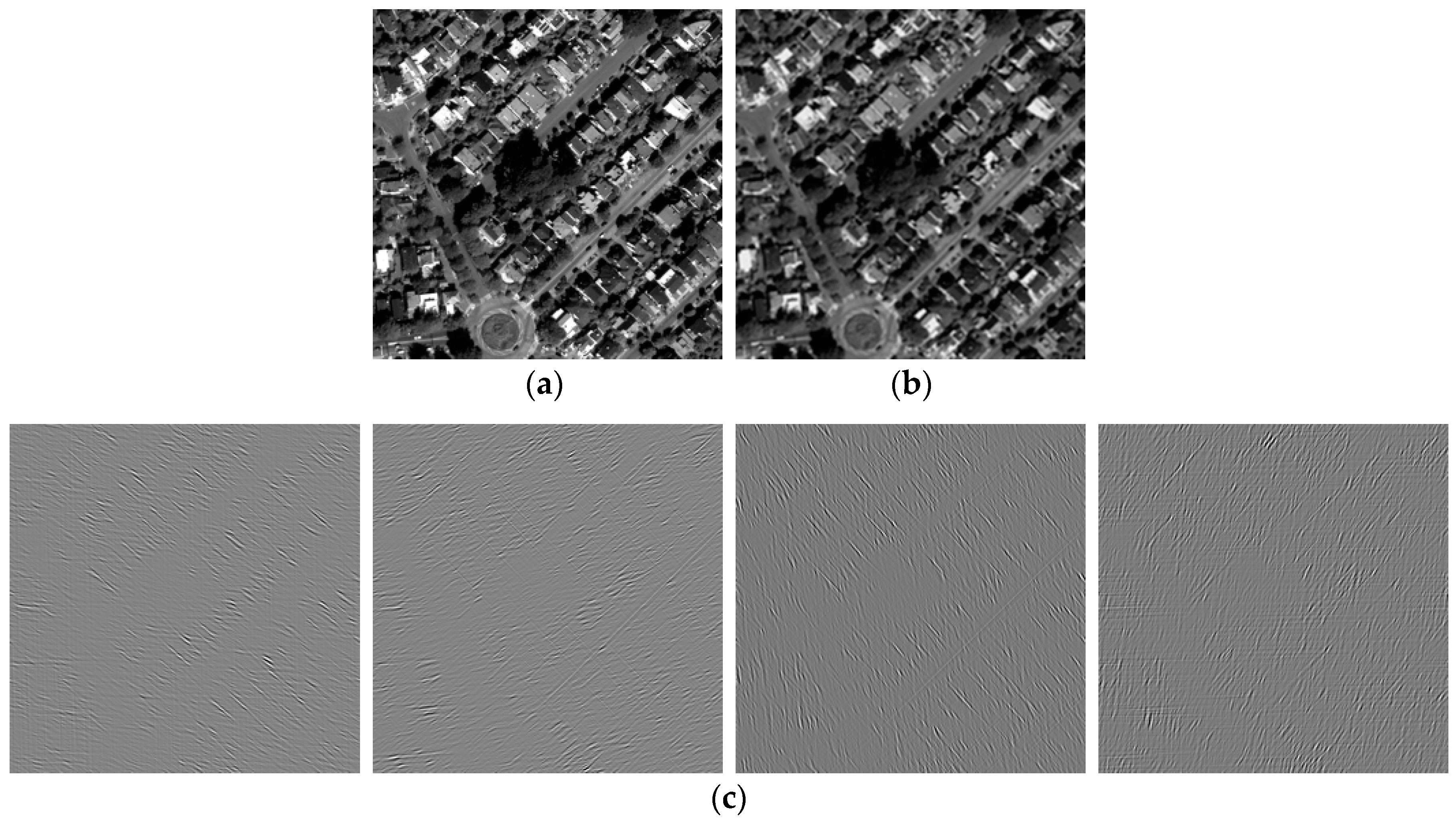
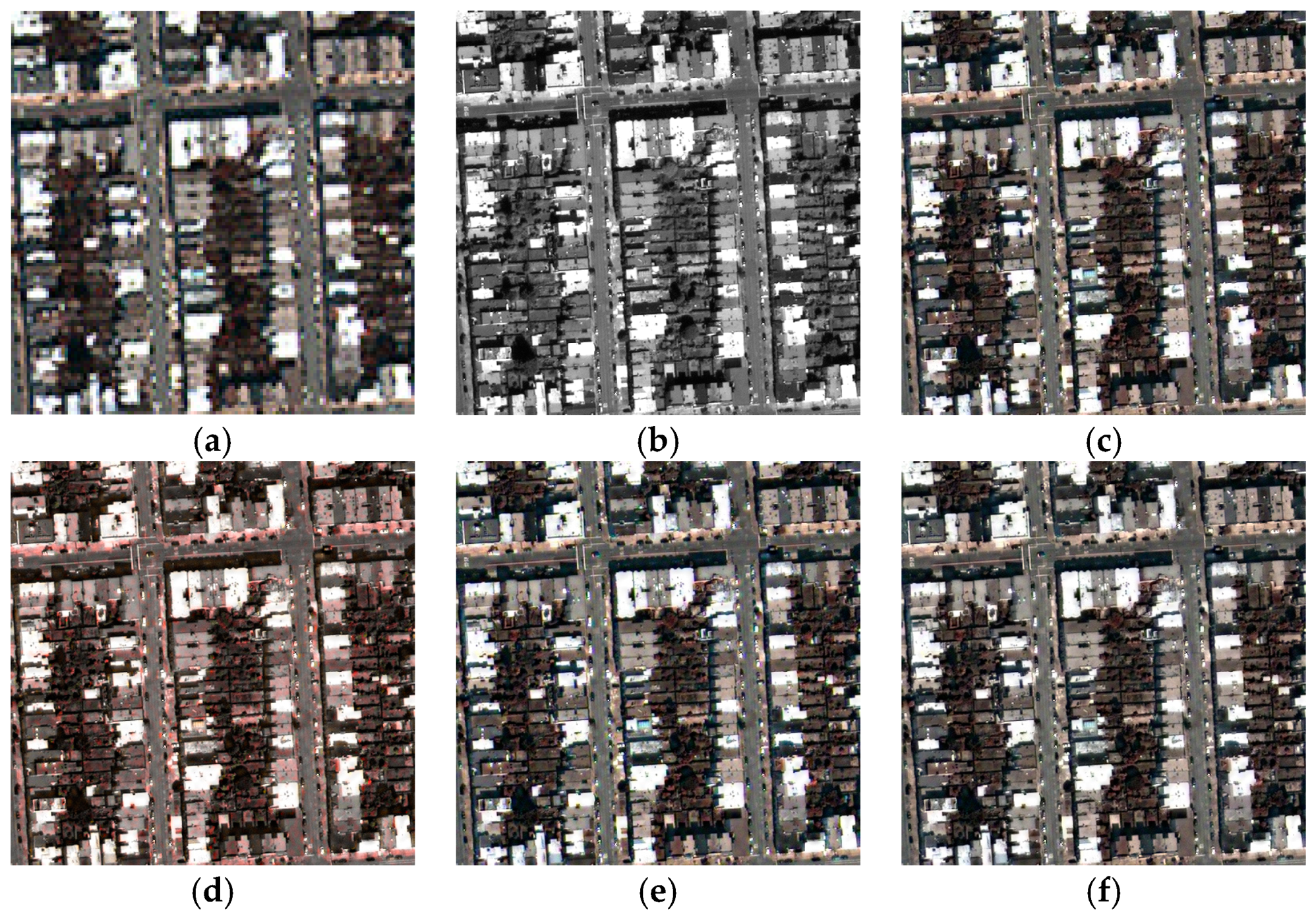
IHS- and PCA-based hybrid methods are classical methods in pan-sharpening, and a great number of studies are based on these two theories. To compare the performance of the IHS- and PCA-based joint frameworks with the proposed matting model framework, we experimented on a WorldView-2 dataset by immobilizing the multiscale transform and used only the simple three-level WT as the multiscale transform tool; the simple average and max approaches are used as the low- and high-frequency coefficient fusion rules, respectively. The fused results and their corresponding objective evaluation are shown in Figure 6 and

Table 3. Objective evaluation of the experimental results shown in Figure 6.

	CC (1)	UIQI (1)	RASE (0)	RMSE (0)	SAM (0)	ERGAS (0)	QNR (1)	Time (s)
IHS	0.9904	0.9897	10.8577	10.9194	6.4446	2.6922	0.9757	0.3461
PCA	0.9960	0.9961	6.1351	6.1699	2.4347	1.5395	0.9883	0.3208
Proposed	0.9962	0.9964	5.9342	5.9679	1.9685	1.4850	0.9970	1.0979

, respectively. The CC, UIQI, RASE, RMSE, SAM, ERGAS, and QNR are utilized to assess the quality of the fused images. The numbers in the brackets refer to the ideal index values.

Figure 6a is the MS image sized $128\times 128$; Figure 6b is the PAN image sized $512\times 512$; Figure 6c is the reference image. Figure 6d–f are the IHS, PCA, and proposed framework fused results. Due to the excellent effects, it is difficult to compare the performance only from visual contrast except that the IHS-fused image exhibits a bit of spectral distortion relative to the reference image. However, from Table 3, the superiority of the proposed framework compared to the IHS- and PCA-based methods can be easily observed in terms of both the spatial and spectral objective quality evaluation indexes. The implementation efficiency is also high, despite the proposed pan-sharpening framework being inferior to the IHS and PCA methods due to the optimization algorithm in the matting model, and this problem will be improved with the development of graphics processing unit (GPU) technology. Thus, the proposed framework is feasible and effective in the pan- sharpening field.

4.4. Comparison with State-of-the-Art Methods

Several experiments have been carried out to compare the pan-sharpening performance of these methods, which include the proposed framework and some existing state-of-the-art approaches. Moreover, the source images acquired by different satellite datasets and different types of land cover were utilized to test the robust performance of the proposed framework. In this part, the proposed framework is respectively combined with DWT (set as experimental, as noted previously) and NSST to compete with the following excellent pan-sharpening approaches, which have for the most part appeared in recent years.

(1)

DWT–SR: DWT and Sparse Representation-based method [26];

(2)

Curvelet: Curvelet transform-based method [27];

(3)

NSST–SR: NSST and Sparse Representation-based method [46];

(4)

GF: Guided Filter-based method [47];

(5)

AWLP: Additive Wavelet Luminance Proportional method, a generalization of AWL [48];

(6)

BFLP: Bilateral Filter Luminance Proportional method [49].

(7)

MM: Matting model and component substitution-based method [33].

(8)

MM–DWT: The proposed framework and DWT-based method.

(9)

MM–NSST: The proposed framework and NSST-based method.

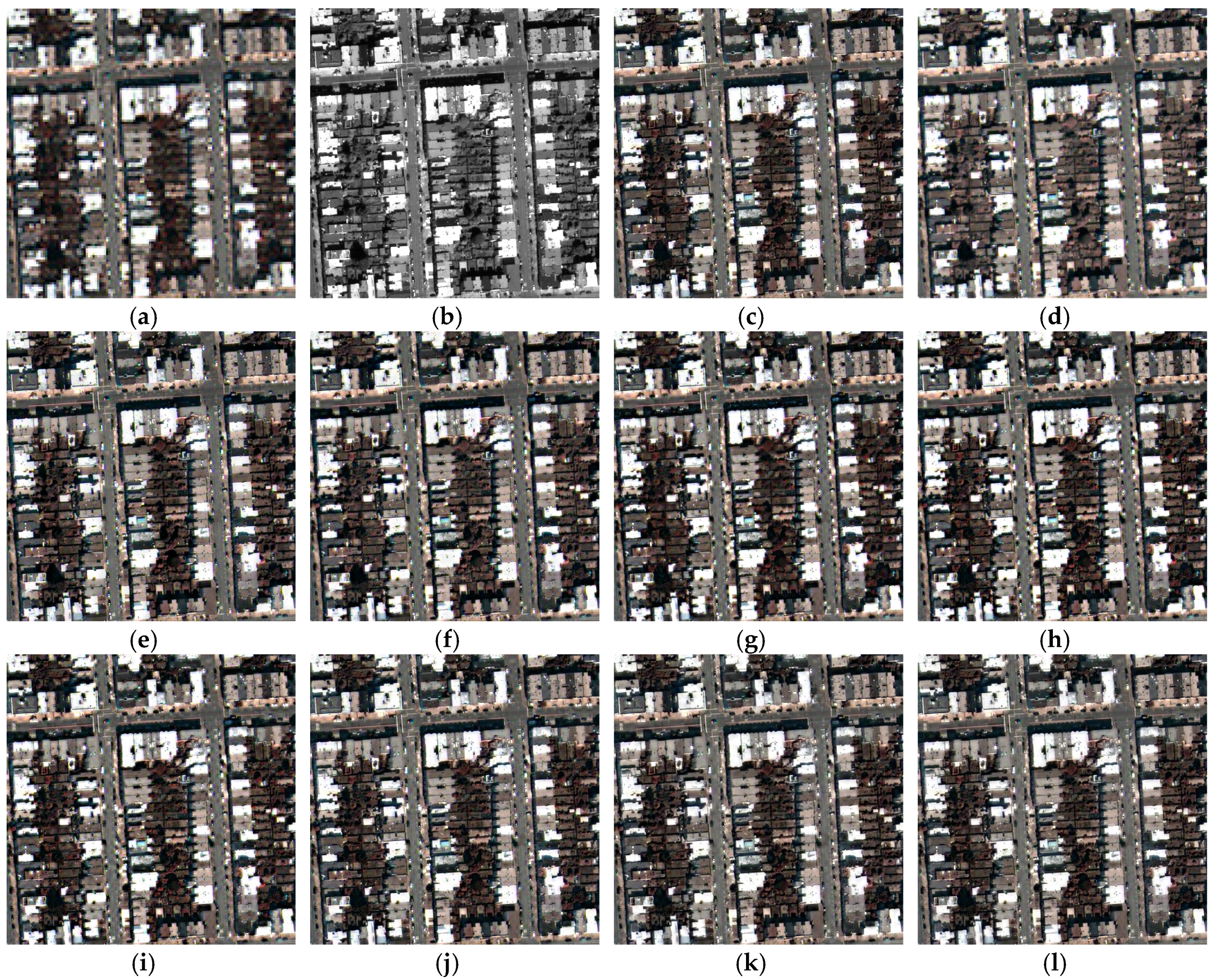
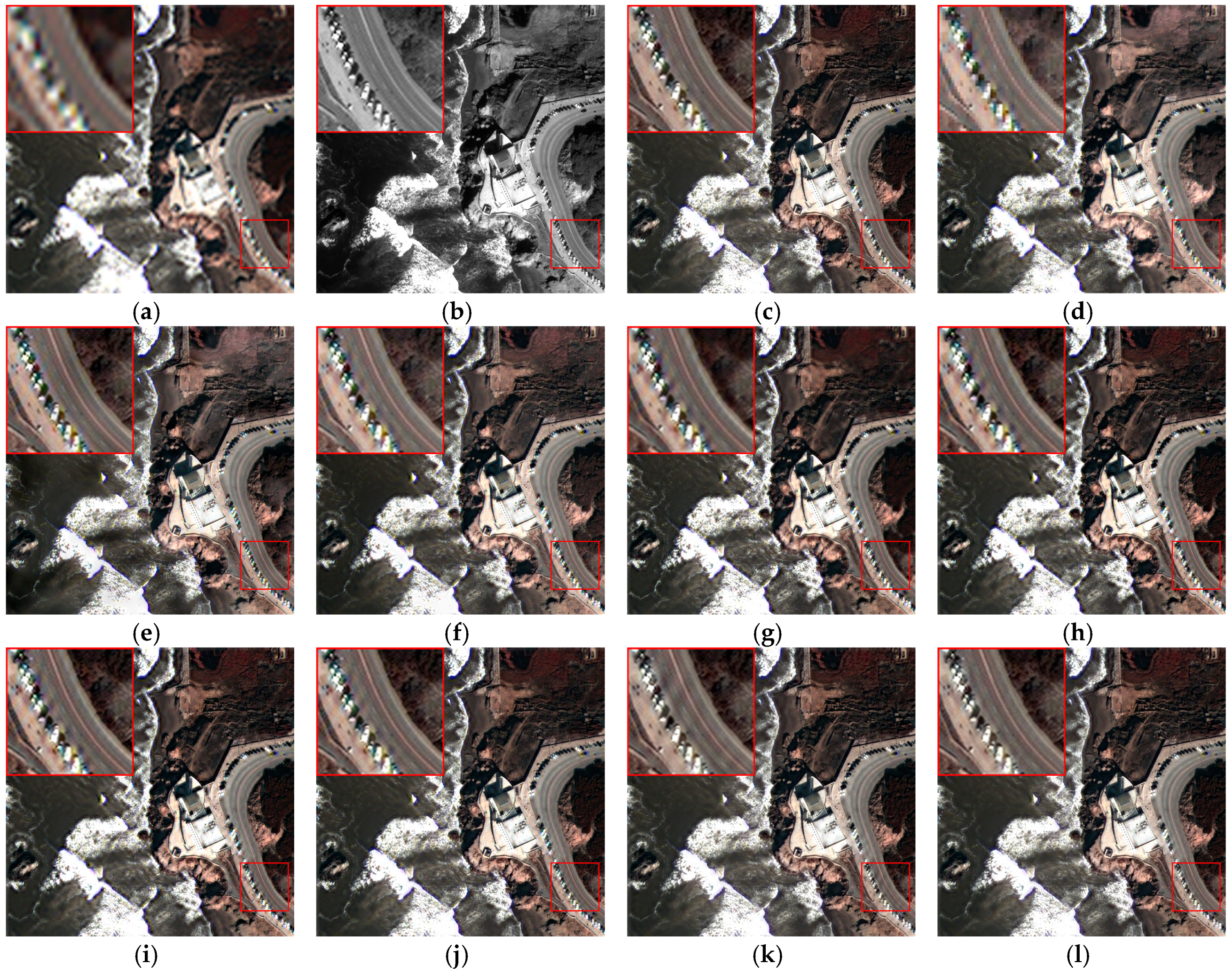
The first group experiment was performed on the WorldViwe-2 datasets coast area. Figure 7 shows the source images and their fusion results; Figure 7a,b are the MS image and PAN image; Figure 7c is the ground truth image; Figure 7d–l are the fusion results of different pan-sharpening methods. To observe the fusion results more clearly, we cut a sub-image placing at the top left corner in the fused images. A visual comparison indicates that the DWT–SR and Curvelet results exhibit spectral distortion phenomena; the result of the NSST–SR method shows improvement, but not remarkably. The GF, AWLP, and BFLP methods obtained better spectral information overall. However, from the sub-images, it is apparent that some serious artifacts occurred around the cars. The fusion results of the MM, MM–DWT, and MM–NSST methods are all close to the reference image, particularly the spectral aspect, which indicates the superiority of the matting model in spectral preservation. Undeniably, the MM–DWT result has spatial distortion in the road area. Due to the productive shift invariance in NSST, the proposed MM–NSST method can overcome the artifacts effectively; thus, apart from the outstanding spectral information, this method can obtain high spatial quality as well.

Table 4. Objective evaluation of the experimental results shown in Figure 7.

Method	DWT–SR	Curvelet	NSST–SR	GF	AWLP	BFLP	MM	MM–DWT	MM–NSST
CC (1)	0.9646	0.9711	0.9856	0.9952	0.9956	0.9961	0.9985	0.9977	0.9986
UIQI (1)	0.9667	0.9753	0.9863	0.9953	0.9955	0.9960	0.9985	0.9978	0.9986
RASE (0)	21.4970	18.0480	12.8259	7.5934	7.4185	6.9464	4.0416	5.1078	4.0004
RMSE (0)	19.4580	16.3362	11.6094	6.8732	6.7149	6.2875	3.6583	4.6233	3.6210
SAM (0)	1.8399	2.0210	1.7476	1.5594	1.5969	1.5584	1.4483	1.5841	1.5503
ERGAS (0)	4.9858	4.4835	3.1999	1.9105	1.8597	1.7410	1.0128	1.2760	0.9994
QNR (1)	0.9788	0.9732	0.9678	0.9909	0.9894	0.9896	0.9960	0.9976	0.9977

presents the objective evaluation results in Figure 7; although the largest SAM value is achieved by the MM method, the proposed MM–NSST method obtains the best values in other indexes as well as the second largest SAM value. In summary, the proposed pan-sharpening framework can obtain outstanding performance in terms of both spatial acquirement and spectral preserving.

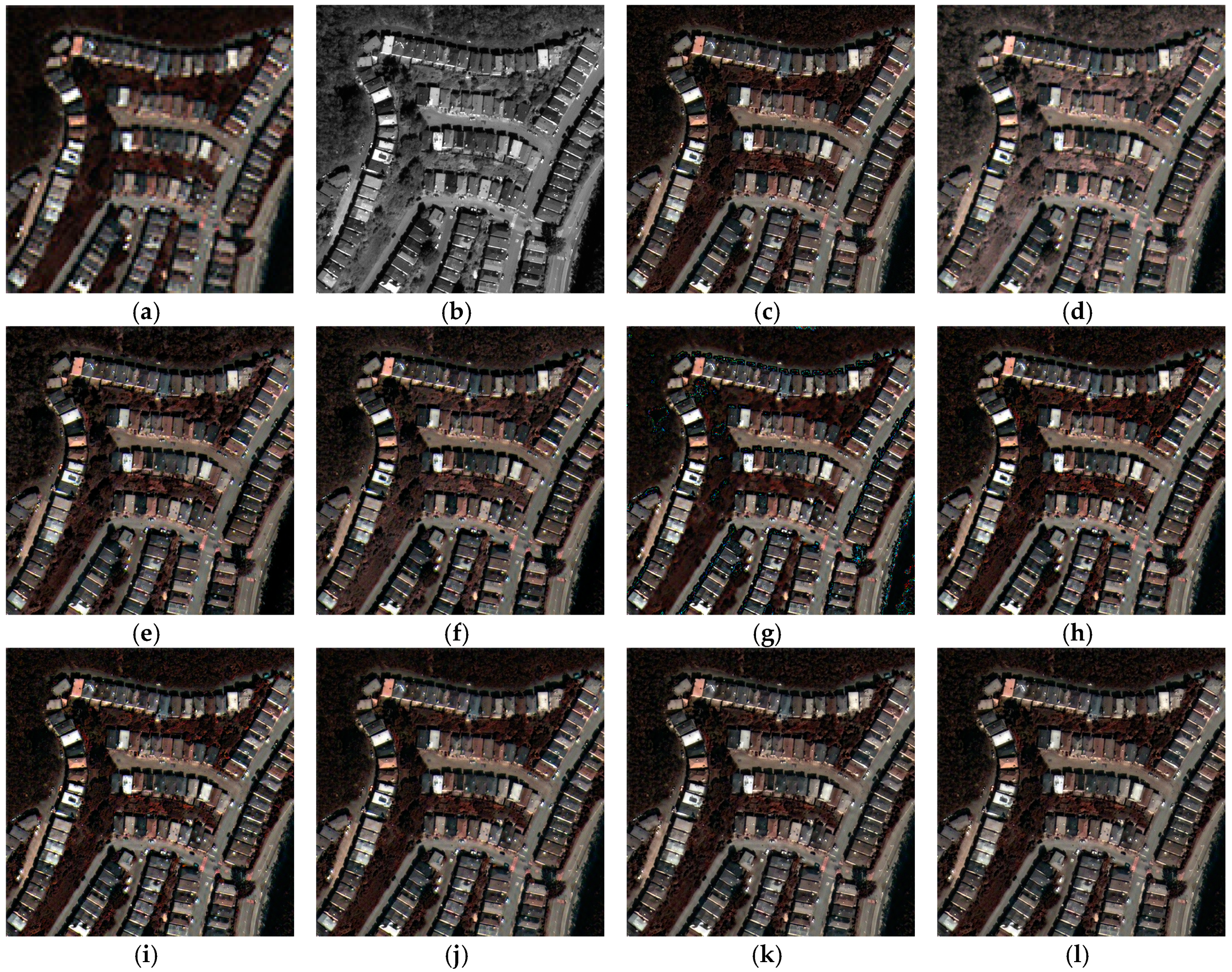
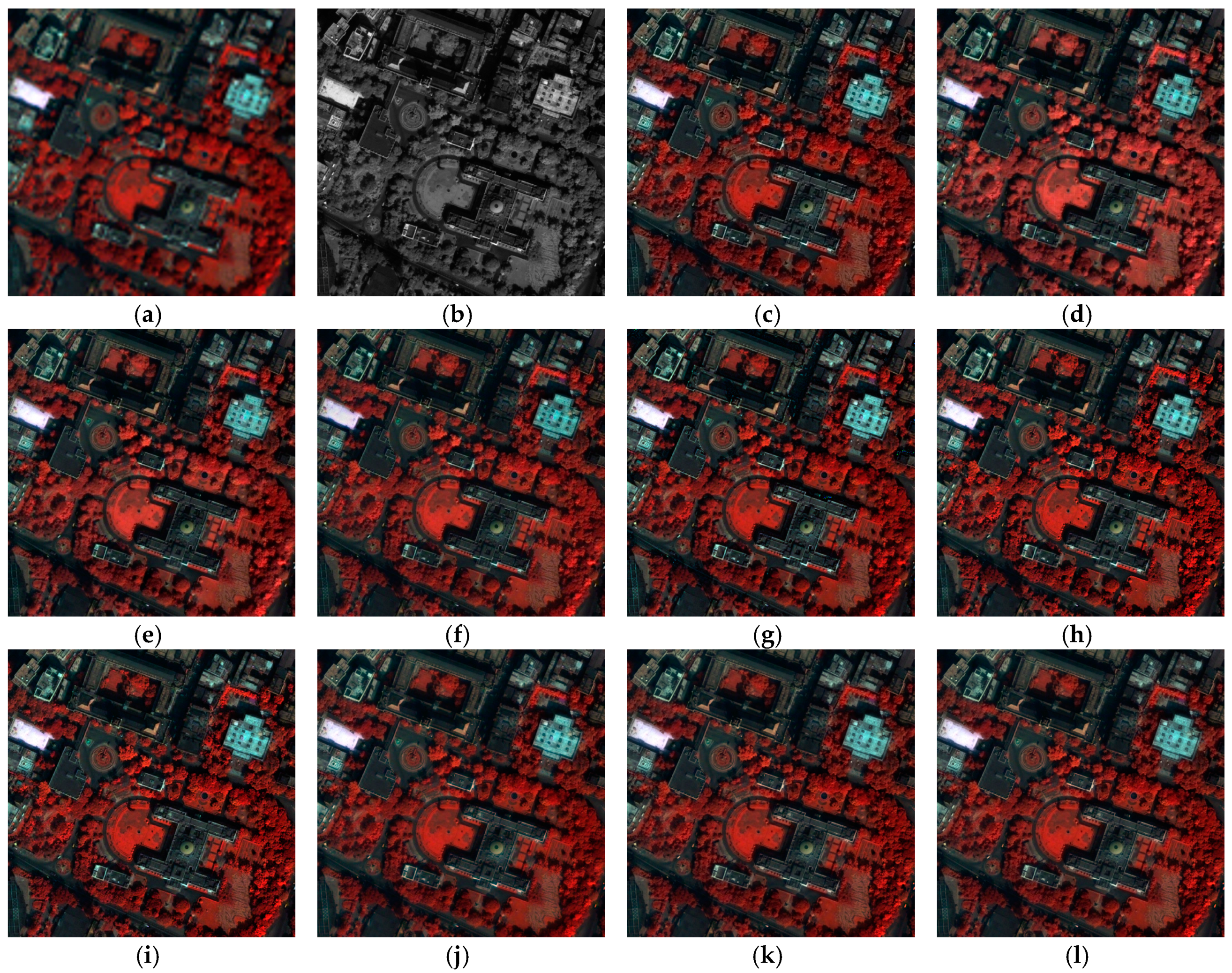
Different land cover types were considered with respect to performance, and the second group experiment was tested on the WorldView-2 datasets with urban land cover. Figure 8a–c are the source MS and PAN images and reference image, respectively. Figure 8d–l and

Table 5. Objective evaluation of the experimental results shown in Figure 8.

Method	DWT–SR	Curvelet	NSST–SR	GF	AWLP	BFLP	MM	MM–DWT	MM–NSST
CC (1)	0.9687	0.9906	0.9918	0.9939	0.9941	0.9946	0.9982	0.9962	0.9983
UIQI (1)	0.9682	0.9912	0.9921	0.9933	0.9932	0.9941	0.9982	0.9964	0.9983
RASE (0)	18.9688	9.3283	8.7783	8.2456	8.3011	7.6844	4.1739	5.9342	4.0474
RMSE (0)	19.0765	9.3813	8.8282	8.2925	8.3483	7.728	4.1976	5.9679	4.0703
SAM (0)	2.2244	2.7249	2.8881	2.5731	2.4821	2.3324	1.9087	1.9685	1.8049
ERGAS (0)	4.3701	2.3355	2.1987	2.0851	2.0879	1.9321	1.0461	1.485	1.0143
QNR (1)	0.9852	0.9864	0.9857	0.9862	0.984	0.9837	0.9968	0.997	0.9976

display the fusion result images and the objective evaluation results of different methods. Spatial and spectral information analyses were performed. Due to this area object’s characteristics, apart from the fusion result of the DWT–SR method suffering from slight spectral distortions and the AWLP, BFLP methods have some degree of spatial blurring, and the fusion results of the other methods obtained fused images with good visual performance, which approximate the reference image. Therefore, there was no obvious comparison with subjective evaluation. However, the objective quality comparison results shown in Table 5 indicate that the proposed method obtained the best values for all evaluation indexes; thus, the proposed method achieves the highest spatial quality while maintaining the best spectral information.

The third group experiment was performed on an uptown area from the WorldView-2 dataset. Usually, suburban areas contain abundant vegetation cover, which is commonly used in spectral contrast. Figure 9a is the low-resolution MS image, and Figure 9c is the high-resolution MS reference image. Using these two MS images as spectral references, we can visually compare the spectral maintaining performance of different pan-sharpening approaches. The spectral distortion of the DWT–SR method is the most serious; the vegetation area in particular is affected, although it obtains preferable spatial quality. The Curvelet and NSST–SR methods show some improvement. The GF method exhibits varying degrees of spectral aberrance and introduces some spectral information that does not exist in the source MS image. The AWLP, BFLP, MM, and proposed methods achieve better progress in spectral maintaining.

Table 6. Objective evaluation of the experimental results shown in Figure 9.

Method	DWT–SR	Curvelet	NSST–SR	GF	AWLP	BFLP	MM	MM–DWT	MM–NSST
CC (1)	0.9009	0.9781	0.9803	0.9651	0.9912	0.9923	0.9963	0.9940	0.9968
UIQI (1)	0.8870	0.9802	0.9815	0.9780	0.9908	0.9920	0.9962	0.9941	0.9967
RASE (0)	50.7517	17.6109	16.7589	23.5971	11.9922	11.1769	7.3060	9.3353	6.8594
RMSE (0)	29.2685	10.1562	9.6649	13.6084	6.9159	6.4457	4.2134	5.3837	3.9558
SAM (0)	4.9788	4.2180	5.0425	5.3581	4.8790	3.9786	3.3136	3.0381	2.7414
ERGAS (0)	9.4432	4.4810	4.1902	5.9943	3.0179	2.8079	1.8717	2.3337	1.7317
QNR (1)	0.9132	0.9803	0.9637	0.9752	0.9788	0.9811	0.9874	0.9954	0.9971

shows the objective quality assessments of this group experiment, from which we can see that the proposed MM–NSST method obtains the best effect compared with other methods.

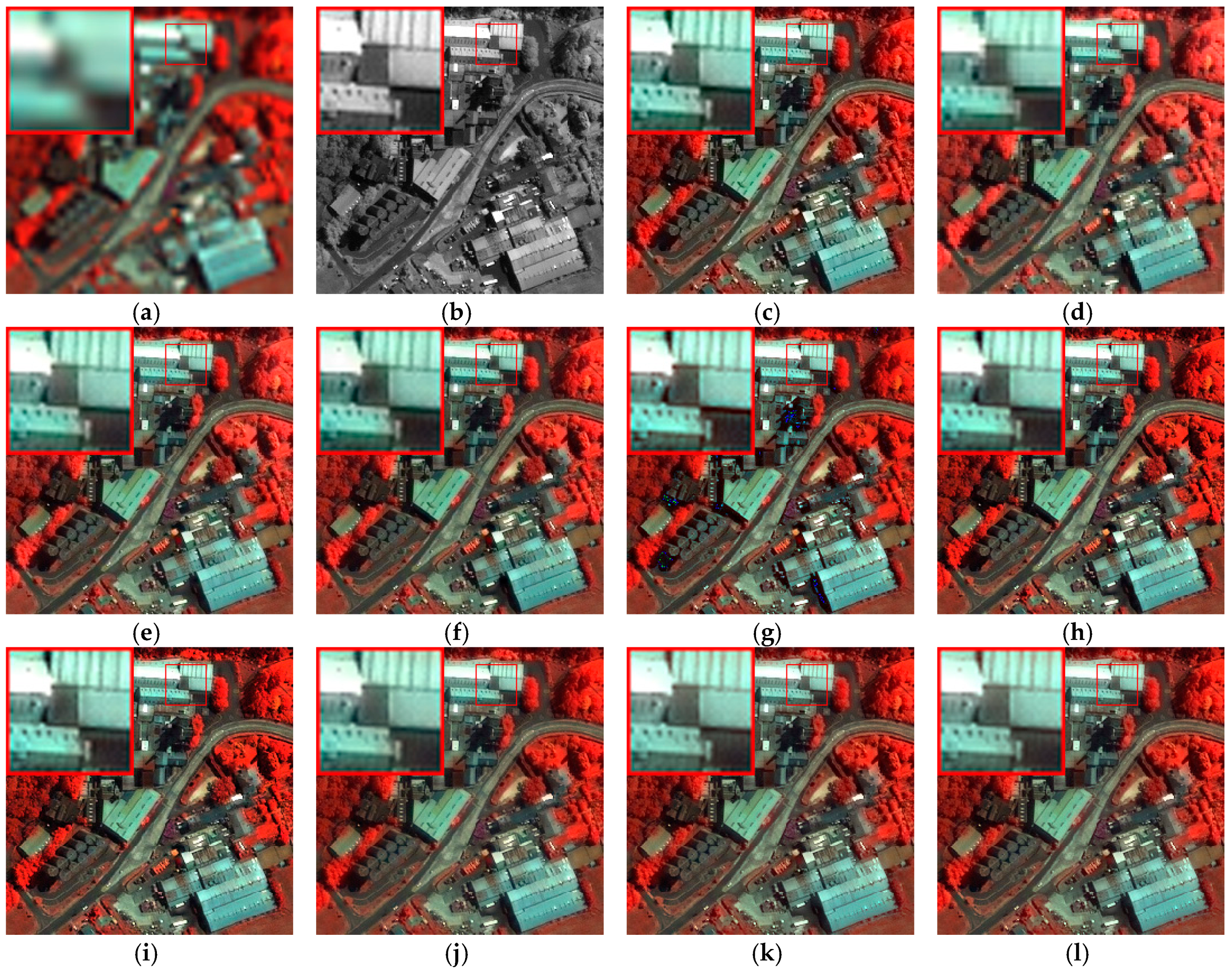
The IKONOS dataset was used in the fourth group experiment to compare the performance of the proposed framework on different satellite images. The MS image of this dataset includes four bands (nir red, red, green, and blue). We used the nir red, green and blue bands for display. Figure 10a,b are the degraded MS image and PAN image; Figure 10c is the original MS image and is used as a reference image. Similarly, we cut the sub-images and placed them at the top left corner in the fused images as well. Compared with the reference image, the fusion performance of the DWT–SR method is unsatisfactory both in the spatial and spectral aspects. The Curvelet and NSST–SR methods improved with respect to the spatial aspect, but the spectral side needs further improvement. The GF method result still suffers from spectral distortion. Other resultant images look similar to the original MS image. The objective evaluation results shown in

Table 7. Objective evaluation of the experimental results shown in Figure 10.

Method	DWT–SR	Curvelet	NSST–SR	GF	AWLP	BFLP	MM	MM–DWT	MM–NSST
CC (1)	0.9590	0.9908	0.9909	0.9830	0.9885	0.9876	0.9897	0.9949	0.9957
UIQI (1)	0.9567	0.9896	0.9882	0.9855	0.9894	0.9889	0.9892	0.9946	0.9952
RASE (0)	21.5995	10.2956	10.4236	12.6101	12.0082	12.5582	9.3684	7.9566	7.5183
RMSE (0)	18.2527	8.7003	8.8085	10.6562	10.1475	10.6123	7.9168	6.7237	6.3534
SAM (0)	4.6338	3.3368	3.3339	6.1866	4.8269	4.9213	3.2161	3.0173	2.9537
ERGAS (0)	5.0735	2.5563	2.6788	3.4344	2.9732	3.0793	2.5574	2.0086	1.8988
QNR (1)	0.9746	0.9835	0.9831	0.9938	0.9905	0.9903	0.9848	0.9908	0.9914

indicate that the proposed MM–NSST method excels in six indexes and the QNR value is the second largest; this is testament to the superiority of our framework on the IKONOS dataset.

The last group dataset used in this paper is obtained from the QuickBird satellite; it also consists of four bands in the MS image. We displayed the three band color images as in the IKONOS set. These experimental data focus on the suburban regions, which have a great deal of vegetation. Thus, it is more convenient for spectral information comparison. From Figure 11, it can be seen that all the pan-sharpening methods achieved decent spatial quality. The DWT–SR and Curvelet methods have slight spectral distortion compared to the reference image, and the spectral aberrance of the GF method result is much better in this dataset. Other methods maintain the spectral information of the MS image effectively.

Table 8. Objective evaluation of the experimental results shown in Figure 11.

Method	DWT–SR	Curvelet	NSST–SR	GF	AWLP	BFLP	MM	MM–DWT	MM–NSST
CC (1)	0.9396	0.9781	0.9861	0.9733	0.9820	0.9832	0.9764	0.9878	0.9881
UIQI (1)	0.9446	0.9800	0.9772	0.9783	0.9844	0.9856	0.9772	0.9873	0.9874
RASE (0)	28.2934	16.2784	15.1285	17.2813	18.6592	15.9732	14.3424	11.7297	11.4370
RMSE (0)	13.0611	7.5146	6.9838	7.9775	8.6136	7.3737	6.6208	5.4148	5.2796
SAM (0)	6.0943	4.8190	4.7804	6.9633	7.2298	6.0668	5.3400	4.5608	4.4763
ERGAS (0)	6.5282	4.1048	3.9693	4.6933	4.3225	3.8882	4.0418	3.1059	3.0550
QNR (1)	0.9289	0.9678	0.9678	0.9762	0.9743	0.9773	0.9596	0.9686	0.9684

shows that the proposed MM–DWT method obtains the best performance in the QNR index and the proposed MM–NSST can obtain the best values in other indexes. Thus, the superiority of the proposed pan-sharpening framework is demonstrated again.

4.5. Contrast on Running Time of Multiscale Transform-Based Methods

In this part, the operating efficiency of the proposed method is analyzed. Because the proposed pan-sharpening framework is based on the multiscale transform, comparison with the non-multiscale transform method is meaningless. Thus, only the multiscale transform-based methods are compared.

Table 9. Running time comparison of the multiscale transform-based methods.

Method	DWT–SR	Curvelet	NSST–SR	MM–DWT	MM–NSST
Time (s)	71.73	1.40	177.29	1.21	54.35

shows a comparison of the average running time of the preceding five groups of the multiscale transform-based methods in part 4.4. It can be seen that the running time of the multiscale transform-based pan-sharpening approaches is mainly decided by the transform method and the fusion rules. Obviously, the SR-based fusion rule is time consuming. Due to the more complex decomposition and reconstruction procedures, the NSST requires more time in multiscale transform image fusion than the DWT and Curvelet approaches, but NSST has been proven effective in the foregoing part. In addition, the proposed framework combined with DWT method is the fastest compared to other multiscale transform-based methods. Meanwhile, it should be noticed that in the previous five groups experiments, this method also achieved the desired performance (particularly for those groups on the IKONOS and QuickBird datasets), although the simplest fusion rules were used. Thus, the proposed framework can simultaneously meet the conditions of satisfaction in efficiency and effectiveness if the appropriate multiscale transform method and fusion rules are utilized.

4.6. Implementation Details

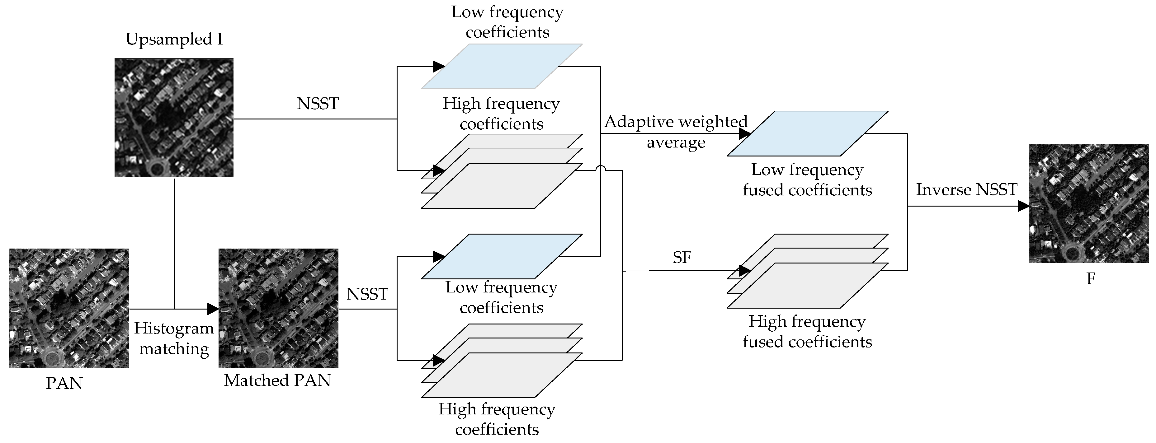
In this section, we provide some implementation details for the proposed method and other comparative methods. All codes are implemented in MATLAB 8.3 (running on a Windows 10 system PC with Intel Core i5-350 3.30-GHz processor and 8-GB memory). All of the resample operations in this paper are bicubic interpolation algorithms. In our method, three-level NSST decomposition with a (30, 40, 60) shearing filter matrix and (2, 3, 4) direction parameters are applied to the upsampled I component and matched PAN image, respectively. The pyramid filter is ‘pyrexc’ wavelet. The parameter $K$ in NSST low-frequency coefficients fusion is 99, and the window size of the local SF in high-frequency coefficient fusion is $3\times 3$. The other pan-sharpening techniques for performance comparison are well known; the experiment parameters in these methods are set as the references.

5. Conclusions

Spectral image pan-sharpening is an important process in remote sensing research and applications. Addressing existing problems in the pan-sharpening area, this paper presented a new pan-sharpening framework by exploiting the matting model and multiscale transform. The proposed framework first obtains the spectral foreground and spectral background of the low- resolution MS image with a matting model, in which the I component of the MS image was used as the alpha channel. Then, the PAN image and the upsampled I component were fused by using a proposed multi-scale image fusion method. The fused image can be used as a new alpha channel to obtain a high-resolution MS image based on a linear combination with upsampled spectral foreground and spectral background images. In this paper, the NSST was introduced in detail as a multi-scale transform example. Through our framework, the PAN and MS image fusion problem was solved. To improve the performance of our method, an adaptive weighted averaging in gradient field rule and a local SF rule were proposed to fuse the low-frequency and high-frequency sub-band coefficients, respectively. Experimental results on different satellite datasets and different land cover certify that the proposed method can achieve superior spatial detail from the PAN image while preserving more spectral information from the MS image compared to some existing pan-sharpening methods. Therefore, the results produced by the proposed method could be better used in the remote sensing applications such as image interpretation, water quality evaluation and vegetated areas research. Importantly, the proposed framework is suitable for any multiscale transform tool to cope with the pan-sharpening research; thus, this framework has bright prospects.

In future works, we would like to improve the effectiveness of the proposed framework by constructing some more powerful multiresolution analysis tools with different Wavelet basis functions. We would also like to extend the application ranges to diverse sensor data, such as optical and radar remote sensing images, thermal infrared and PAN images. Moreover, as in most pan-sharpening literature, we used completely registered satellite images for experiments. We plan to collect some datasets with temporal and instrumental change, and analyze the robustness of the proposed framework on them.

References

1. Zhang, H.; Huang, B. A new look at image fusion methods from a Bayesian perspective. Remote Sens. 2015, 7, 6828–6861. [Google Scholar] [CrossRef]
2. Aiazzi, B.; Alparone, L.; Baronti, S.; Carla, R.; Garzelli, A.; Santurri, L. Sensitivity of pansharpening methods to temporal and instrumental changes between multispectral and panchromatic data sets. IEEE Trans. Geosci. Remote Sens. 2017, 50, 308–319. [Google Scholar] [CrossRef]
3. Hou, L.; Zhang, X. Pansharpening image fusion using cross-channel correlation: A framelet-based approach. J. Math. Imaging Vis. 2016, 55, 36–49. [Google Scholar] [CrossRef]
4. Selva, M.; Aiazzi, B.; Butera, F.; Chiarantini, L.; Baronti, S. Hyper-sharpening: A first approach on SIM-GA data. IEEE J. Sel. Top. Appl. Earth Obs. Remote Sens. 2015, 8, 3008–3024. [Google Scholar] [CrossRef]
5. Vivone, G.; Alparone, L.; Chanussot, J.; Mura, M.; Garzelli, A.; Licciardi, G.; Restaino, R.; Wald, L. A critical comparison among pansharpening algorithms. IEEE Trans. Geosci. Remote Sens. 2014, 53, 2565–2586. [Google Scholar] [CrossRef]
6. Jelének, J.; Kopačková, V.; Koucká, L.; Mišurec, J. Testing a modified PCA-based sharpening approach for image fusion. Remote Sens. 2016, 8, 1–25. [Google Scholar] [CrossRef]
7. Tu, T.; Huang, P.; Hung, C.; Chang, C. A fast intensity-hue-saturation fusion technique with spectral adjustment for IKONOS imagery. IEEE Geosci. Remote Sens. Lett. 2004, 1, 309–312. [Google Scholar] [CrossRef]
8. Rahmani, S.; Strait, M.; Merkurjev, D.; Moeller, M.; Wittman, T. An adaptive IHS Pan-sharpening method. IEEE Geosci. Remote Sens. Lett. 2010, 7, 746–750. [Google Scholar] [CrossRef]
9. Laben, C.; Brower, B. Process for Enhancing the Spatial Resolution of Multispectral Imagery Using Pan-Sharpening. U.S. Patent 6,011,875, 4 January 2000. [Google Scholar]
10. He, X.; Condat, L.; Bioucas-Dias, J.; Chanussot, J.; Xia, J. A new pansharpening method based on spatial and spectral sparsity priors. IEEE Trans. Image Process. 2014, 23, 4160–4174. [Google Scholar] [CrossRef] [PubMed]
11. Palsson, F.; Sveinsson, J.R.; Ulfarsson, M.O.; Benediktsson, J.A. MTF-based deblurring using a wiener filter for CS and MRA pansharpening methods. IEEE J. Sel. Top. Appl. Earth Obs. Remote Sens. 2016, 9, 2255–2269. [Google Scholar] [CrossRef]
12. Li, S.; Yang, B. A new pan-sharpening method using a compressed sensing technique. IEEE Trans. Geosci. Remote Sens. 2011, 49, 738–746. [Google Scholar] [CrossRef]
13. Zhu, X.; Grohnfeldt, C.; Bamler, R. Exploiting joint sparsity for pansharpening: The J-sparseFI algorithm. IEEE Trans. Geosci. Remote Sens. 2016, 54, 738–746. [Google Scholar] [CrossRef]
14. Alparone, L.; Baronti, S.; Aiazzi, B.; Garzelli, A. Spatial methods for multispectral pansharpening: Multiresolution analysis demystified. IEEE Trans. Geosci. Remote Sens. 2016, 54, 2563–2576. [Google Scholar] [CrossRef]
15. Shi, Y.; Yang, X.; Cheng, T. Pansharpening of multispectral images using the nonseparable framelet lifting transform with high vanishing moments. Inf. Fusion 2014, 20, 213–224. [Google Scholar] [CrossRef]
16. Aiazzi, B.; Alparone, L.; Baronti, S.; Garzelli, A. Context-driven fusion of high spatial and spectral resolution images based on oversampled multiresolution analysis. IEEE Trans. Geosci. Remote Sens. 2002, 40, 2300–2312. [Google Scholar] [CrossRef]
17. Petrovic, A.; Xydeas, C. Gradient-based multiresolution image fusion. IEEE Trans. Image Process. 2004, 13, 228–237. [Google Scholar] [CrossRef] [PubMed]
18. Li, S.; Kwok, J.; Wang, Y. Using the discrete Wavelet frame transform to merge Landsat TM and SPOT panchromatic images. Inf. Fusion 2002, 3, 17–23. [Google Scholar] [CrossRef]
19. Ioannidou, S.; Karathanassi, V. Investigation of the dual-tree complex and shift-invariant discrete Wavelet transforms on Quickbird image fusion. IEEE Geosci. Remote Sens. Lett. 2007, 4, 166–170. [Google Scholar] [CrossRef]
20. Ghahremani, M.; Ghassemian, H. Remote sensing image fusion based on Curvelets and ICA. Int. J. Remote Sens. 2015, 36, 4131–4143. [Google Scholar] [CrossRef]
21. Metwalli, M.; Nasr, A.; Faragallah, O.; EI-Rabaie, E.; Abbas, A.; Alshebeili, S.; EI-Samie, F. Efficient pan-sharpening of satellite images with the Contourlet transform. Int. J. Remote Sens. 2014, 35, 1979–2002. [Google Scholar] [CrossRef]
22. Labate, D.; Lim, W.; Kutyniok, G.; Weiss, G. Sparse multidimensional representation using Shearlets. SPIE Proc. 2005, 5914, 254–262. [Google Scholar]
23. Hallabia, H.; Kallel, A.; Hamida, A.; Hegarat-Mascle, S. High spectral quality pansharpening approach based on MTF-matched filter banks. Multidimens. Syst. Signal Process. 2016, 4, 1–31. [Google Scholar] [CrossRef]
24. Yang, Y.; Wan, W.; Huang, S.; Yuan, F.; Yang, S.; Que, Y. Remote sensing image fusion based on adaptive IHS and multiscale guided filter. IEEE Access. 2016, 4, 4573–4582. [Google Scholar] [CrossRef]
25. Licciardi, G.; Vivone, G.; Mura, M.D. Multi-resolution analysis techniques and nonlinear PCA for hybrid pansharpening applications. Multidimens. Syst. Signal Process. 2016, 27, 807–830. [Google Scholar] [CrossRef]
26. Cheng, J.; Liu, H.; Liu, T.; Wang, F.; Li, H. Remote sensing image fusion via Wavelet transform and sparse representation. ISPRS J. Photogramm. Remote Sens. 2015, 104, 158–173. [Google Scholar] [CrossRef]
27. Dong, L.; Yang, Q.; Wu, H.; Xiao, H.; Xu, M. High quality multi-spectral and panchromatic image fusion technologies based on Curvelet transform. Neurocomputing 2015, 159, 268–274. [Google Scholar] [CrossRef]
28. Shah, V.; Younan, N.; King, R. An efficient pan-sharpening method via a combined adaptive PCA approach and contourlets. IEEE Trans. Geosci. Remote Sens. 2008, 46, 1323–1335. [Google Scholar] [CrossRef]
29. Ourabia, S.; Smara, Y. A new pansharpening approach based on nonsubsampled Contourlet transform using enhanced PCA applied to SPOT and ALSAT-2A satellite image. J. Indian Soc. Remote Sens. 2016, 44, 665–674. [Google Scholar] [CrossRef]
30. Cunha, A.; Zhou, J.; Do, M. The nonsubsampled Contourlet transform: Theory, design and application. IEEE Trans. Image Process. 2006, 15, 3089–3101. [Google Scholar] [CrossRef] [PubMed]
31. Yin, M.; Liu, W.; Zhao, X.; Yin, Y.; Guo, Y. A novel image fusion algorithm based on nonsubsampled Shearlet transform. Opt. Int. J. Light Electron Opt. 2014, 125, 2274–2282. [Google Scholar] [CrossRef]
32. Levin, A.; Lischinski, D.; Weiss, Y. A closed form solution to natural image matting. IEEE Trans. Pattern Anal. Mach. Intell. 2008, 30, 228–242. [Google Scholar] [CrossRef] [PubMed]
33. Kang, X.; Li, S.; Benediktsson, J. Pansharpening with matting model. IEEE Trans. Geosci. Remote Sens. 2014, 52, 5088–5099. [Google Scholar] [CrossRef]
34. Gao, G.; Xu, L.; Feng, D. Multi-focus image fusion based on non-subsampled Shearlet transform. IET Image Process. 2013, 7, 633–639. [Google Scholar]
35. Masi, G.; Cozzolino, D.; Verdoliva, L.; Scarpa, G. Pansharpening by convolutional neural networks. Remote Sens. 2016, 8, 1–22. [Google Scholar] [CrossRef]
36. WorldView-2 Datasets. Available online: http://www.datatang.com/data/43234 (accessed on 17 September 2015). (In Chinese).
37. IKONOS Datasets. Available online: http://www.isprs.org/data/ikonos_hobart/default.aspx (accessed on 22 March 2016).
38. QuickBird Datasets. Available online: http://www.glcf.umiacs.umd.edu/data/ (accessed on 12 July 2016).
39. Wald, L.; Ranchin, T.; Mangolini, M. Fusion of satellite images of different spatial resolutions: Assessing the quality of resulting images. Photogramm. Eng. Remote Sens. 1997, 63, 691–699. [Google Scholar]
40. Wang, Z.; Bovik, A. A universal image quality index. IEEE Signal Process. Lett. 2002, 9, 81–84. [Google Scholar] [CrossRef]
41. Yang, Y.; Tong, S.; Huang, S.; Lin, P. Multifocus image fusion based on NSCT and focused area detection. IEEE Sens. J. 2015, 15, 2824–2838. [Google Scholar]
42. Ranchin, T.; Wald, L. Fusion of high spatial and spectral resolution images: The ARSIS concept and its implementation. Photogramm. Eng. Remote Sens. 2000, 66, 49–61. [Google Scholar]
43. Yuhas, R.; Goetz, A.; Boardman, J. Discrimination among Semi-Arid Landscape Endmembers Using the Spectral Angle Mapper (SAM) Algorithm. Available online: https://ntrs.nasa.gov/search.jsp?R=19940012238 (accessed on 9 February 2017).
44. Wald, L. Quality of high resolution synthesised images: Is there a simple criterion? In Proceedings of the 3rd Conference “Fusion Earth Data: Merging Point Measurement, Raster Maps and Remotely Sensed Images”, Sophia Antipolis, France, 26–28 January 2000. [Google Scholar]
45. Alparone, L.; Aiazzi, B.; Baronti, S.; Garzelli, A.; Nencini, F.; Selva, M. Multispectral and panchromatic data fusion assessment without reference. Photogramm. Eng. Remote Sens. 2008, 74, 193–200. [Google Scholar] [CrossRef]
46. Moonon, A.; Hu, J.; Li, S. Remote sensing image fusion method based on nonsubsampled Shearlet transform and sparse representation. Sens. Imaging Int. J. 2015, 16, 1–18. [Google Scholar] [CrossRef]
47. Jameel, A.; Riaz, M.; Ghafoor, A. Guided filter and IHS-based pan-sharpening. IEEE Sens. J. 2015, 16, 192–194. [Google Scholar] [CrossRef]
48. Otazu, X.; González-Audícana, M.; Fors, O.; Núñez, J. Introduction of sensor spectral response into image fusion methods. Application to wavelet-based methods. IEEE Trans. Geosci. Remote Sens. 2005, 43, 2376–2385. [Google Scholar] [CrossRef]
49. Kaplan, N.; Erer, I. Bilateral filtering-based enhanced pansharpening of multispectral satellite images. IEEE Geosci. Remote Sens. Lett. 2014, 11, 1941–1945. [Google Scholar] [CrossRef]
Figure 1. An example of image matting: (a) QuickBird multispectral (MS) image; (b) alpha channel; (c) foreground image; (d) background image; (e) I component of the MS image; (f) foreground color; (g) background color.
Remotesensing 09 00391 g001
Figure 2. Three-level multiscale and multidirectional decomposition of the nonsubsampled Shearlet transform (NSST).
Remotesensing 09 00391 g002
Figure 3. Decomposition diagram of NSST: (a) WorldView-2 satellite image; (b) low-frequency image; (c) high-frequency images.
Remotesensing 09 00391 g003
Figure 4. The schematic diagram of the proposed pan-sharpening framework.
Remotesensing 09 00391 g004
Figure 5. The flow chart of upsampled I and matched panchromatic (PAN) image fusion using NSST.
Remotesensing 09 00391 g005
Figure 6. The fused results of the intensity-hue-saturation (IHS), PCA- and matting model-based methods on WorldView-2 dataset: (a) MS image; (b) PAN image; (c) reference image; (d) IHS–wavelet transform (WT) result; (e) PCA–WT result; (f) proposed matting model–WT result.
Remotesensing 09 00391 g006
Figure 7. The fusion results of WorldView-2 datasets on coast area: (a) MS image; (b) PAN image; (c) reference image; (d) DWT–Sparse Representation (SR); (e) Curvelet; (f) NSST–SR; (g) Guided Filter (GF); (h) Additive Wavelet Luminance Proportional (AWLP); (i) Bilateral Filter Luminance Proportional (BFLP); (j) Matting Model (MM); (k) MM–DWT; (l) MM–NSST.
Remotesensing 09 00391 g007
Figure 8. The fusion results of WorldView-2 datasets on urban area: (a) MS image; (b) PAN image; (c) reference image; (d) DWT–Sparse Representation (SR); (e) Curvelet; (f) NSST–SR; (g) Guided Filter (GF); (h) Additive Wavelet Luminance Proportional (AWLP); (i) Bilateral Filter Luminance Proportional (BFLP); (j) Matting Model (MM); (k) MM–DWT; (l) MM–NSST.
Remotesensing 09 00391 g008
Figure 9. The fusion results of WorldView-2 datasets on an uptown area: (a) MS image; (b) PAN image; (c) reference image; (d) DWT–Sparse Representation (SR); (e) Curvelet; (f) NSST–SR; (g) Guided Filter (GF); (h) Additive Wavelet Luminance Proportional (AWLP); (i) Bilateral Filter Luminance Proportional (BFLP); (j) Matting Model (MM); (k) MM–DWT; (l) MM–NSST.
Remotesensing 09 00391 g009
Figure 10. The fusion results on the IKONOS dataset: (a) MS image; (b) PAN image; (c) reference image; (d) DWT–Sparse Representation (SR); (e) Curvelet; (f) NSST–SR; (g) Guided Filter (GF); (h) Additive Wavelet Luminance Proportional (AWLP); (i) Bilateral Filter Luminance Proportional (BFLP); (j) Matting Model (MM); (k) MM–DWT; (l) MM–NSST.
Remotesensing 09 00391 g010
Figure 11. The fusion results on the QuickBird dataset: (a) MS image; (b) PAN image; (c) reference image; (d) DWT–Sparse Representation (SR); (e) Curvelet; (f) NSST–SR; (g) Guided Filter (GF); (h) Additive Wavelet Luminance Proportional (AWLP); (i) Bilateral Filter Luminance Proportional (BFLP); (j) Matting Model (MM); (k) MM–DWT; (l) MM–NSST.
Remotesensing 09 00391 g011