
Detection of Absorbing Aerosol Using Single Near-UV Radiance Measurements from a Cloud and Aerosol Imager


1
Department of Atmospheric Sciences, Yonsei University, 50 Yonsei-ro, Seodaemun-gu, Seoul 03722, Korea
2
Harvard Smithonian Center for Astrophysics, Harvard University, Cambridge, MA 02138, USA
3
School of Earth and Environmental Sciences, Seoul National University, 1 Gwanak-ro, Gwanak-gu, Seoul 08826, Korea
4
Goddard Space Flight Center, National Aeronautics and Space Administration, Greenbelt, MD 20771, USA
5
Earth System Science Interdisciplinary Center, University of Maryland, College Park, MD 20740, USA
*
Author to whom correspondence should be addressed.
Remote Sens. 2017, 9(4), 378; https://doi.org/10.3390/rs9040378
Submission received: 28 November 2016
/
Revised: 21 March 2017
/
Accepted: 24 March 2017
/
Published: 18 April 2017
Abstract
:The Ultra-Violet Aerosol Index (UVAI) is a practical parameter for detecting aerosols that absorb UV radiation, especially where other aerosol retrievals fail, such as over bright surfaces (e.g., deserts and clouds). However, typical UVAI retrieval requires at least two UV channels, while several satellite instruments, such as the Thermal And Near infrared Sensor for carbon Observation Cloud and Aerosol Imager (TANSO-CAI) instrument onboard a Greenhouse gases Observing SATellite (GOSAT), provide single channel UV radiances. In this study, a new UVAI retrieval method was developed which uses a single UV channel. A single channel aerosol index (SAI) is defined to measure the extent to which an absorbing aerosol state differs from its state with minimized absorption by aerosol. The SAI qualitatively represents absorbing aerosols by considering a 30-day minimum composite and the variability in aerosol absorption. This study examines the feasibility of detecting absorbing aerosols using a UV-constrained satellite, focusing on those which have a single UV channel. The Vector LInearized pseudo-spherical Discrete Ordinate Radiative Transfer (VLIDORT) was used to test the sensitivity of the SAI and UVAI to aerosol optical properties. The theoretical calculations showed that highly absorbing aerosols have a meaningful correlation with SAI. The retrieved SAI from OMI and operational OMI UVAI were also in good agreement when UVAI values were greater than 0.7 (the absorption criteria of UVAI). The retrieved SAI from the TANSO-CAI data was compared with operational OMI UVAI data, demonstrating a reasonable agreement and low rate of false detection for cases of absorbing aerosols in East Asia. The SAI retrieved from TANSO-CAI was in better agreement with OMI UVAI, particularly for the values greater than the absorbing threshold value of 0.7.
1. Introduction
An accurate estimation of aerosol radiative forcing requires detailed information on aerosol amounts (e.g., maps of aerosol optical depth, AOD) and aerosol characteristics, such as size, composition, and optical properties, especially absorption and scattering [1,2,3]. The types of aerosols identified by satellite observations are an important issue in the evaluation of climate forcing, because aerosol radiative effects significantly vary from one type to another. Generally, aerosols have been classified into four major types in satellite observations: soil dust, carbonaceous, sulfate, and sea salt [4,5], where their representative particle sizes and radiation absorptivity are quite different. Soil dust particles, for example, are large in size and absorb significant amounts of radiation, especially at ultraviolet (UV) and blue wavelengths, while sulfate aerosol particles are small in size and do not absorb radiation in the UV and visible wavelengths. Although carbonaceous aerosols are complicated in their chemical and optical properties, they are commonly recognized as strongly absorbing (as are soot particles) in UV wavelengths [5,6].
Algorithms for identifying aerosol types from satellite observations have been developed, based on the theoretical characteristics of each satellite’s instrument wavelength channel. The UV wavelengths from satellite observations are helpful for detecting absorbing aerosols and are insensitive to aerosol phase function effects, although they are insensitive to aerosol in the boundary layer, as discussed in Li et al. [7]. Herman et al. [8] successfully detected absorbing aerosols using a UV Aerosol Index (UVAI), whereby soil dust and biomass-burning (carbonaceous) aerosols strongly absorb UV and blue radiation. The strong light absorptivity of such aerosols was also reported by Dubovik et al. [9], who used aerosol inversion products from the ground-based Aerosol Robotic Network (AERONET) measurements. The UVAI is estimated by comparing the two channel near-UV radiances, where trace gas absorption is relatively small, based on the hypothesis that their albedo differences are negligible [10]. The UVAI algorithm has a strong advantage of being applicable over bright surfaces, such as desert and cloud, where many other aerosol inversion products are typically not available.
The UVAI has often been used with the Angstrom Exponent (AE), which provides information on aerosol particle size. Higurashi and Nakajima [11] and Kaufman et al. [12] retrieved the AE using two-channel visible radiances at 0.64 and 0.83 μm. Subsequently, Higurashi and Nakajima [4] developed a four-channel algorithm to classify aerosols into four major types (soil dust, carbonaceous, sulfate, and sea salt), using the four visible channel data of the Sea-Viewing Wide Field-of-View Sensor (SeaWiFS) over the ocean. This algorithm has the advantage of classifying aerosol types from simultaneous measurements at four wavelengths (412, 443, 670, 865 nm) in near real-time. Jeong and Li [13] developed an aerosol classification algorithm by utilizing two instruments: a Total Ozone Mapping Spectrometer (TOMS) and an Advanced Very High Resolution Radiometer (AVHRR). The aerosol size information (AE) from the visible channel of the AVHRR was combined with the aerosol absorption (UVAI) from TOMS, to infer the aerosol types of biomass burning, pollution, dust, sea salt, and a mixture of different types. Kim et al. [5] developed the MODIS-OMI algorithm (MOA), which uses the Moderate Resolution Imaging Spectroradiometer (MODIS) and the Ozone Monitoring Instrument (OMI), and evaluated the consistency between two different aerosol classification algorithms. This algorithm was purely designed to classify aerosols and it uses standard products including MODIS AOD, Fine Mode Fraction (FMF), and OMI UVAI.
UVAI is an important parameter for assessing aerosol absorption and type, but is only available when instruments have more than two UV channels. However, some satellite instruments only have a single UV channel, such as the Thermal And Near infrared Sensor for carbon Observation Cloud and Aerosol Imager (TANSO-CAI) of the Greenhouse gases Observing SATellite (GOSAT). The information on the aerosol type is significantly important for the GOSAT, which aims at retrieving the concentration of greenhouse gas, CO2. Jung et al. [14] reported that incorrect information on the aerosol type can lead to significant errors in CO2 retrievals up to 3 ppm. Although the UVAI can be obtained from other instruments such as the OMI, spatial and temporal collocation results in low information availability. In addition, since OMI has a coarser pixel resolution (13 × 24 km2) than TANSO-CAI (500 × 500 m2), the distinction between absorbing aerosol and non-absorbing aerosol at high resolutions becomes erroneous, which also leads to errors in AOD, CO2, and relevant products.
In this study, we developed an algorithm to discern absorbing aerosol signals using one UV radiance channel, named the Single UV channel Aerosol Index (SAI). The underlying physical principle of SAI is different from that of UVAI. The advantage of the SAI algorithm is its adaptability to satellite platforms with one UV channel. This raises the possibility of distinguishing aerosol absorption through the instruments themselves, and therefore enables us to expand the analysis to include past satellite data for climate research. Moreover, particularly for GOSAT, by providing better information on aerosol absorption from TANSO-CAI, the CO2 retrievals can be improved. The remainder of this manuscript is organized as follows. The instruments used in this study are summarized in Section 2 and a theoretical sensitivity analysis test of UVAI and SAI are presented in Section 3, before the development of an algorithm using satellite instruments. In Section 4, several empirical models of SAI are analyzed to find the best empirical SAI (Section 4.1), and the best SAI empirical model is adapted to the OMI (Section 4.2) and TANSO-CAI (Section 4.3) instruments. Finally, the conclusions are presented in Section 5.
2. Data
2.1. OMI
To test the feasibility of the SAI algorithm, we first applied it to OMI (Section 4.1 and Section 4.2). OMI has hyperspectral bands in the UV and visible (270–500 nm) regions, with a spectral resolution of ~0.5 nm. OMI is a spectrograph onboard the Earth Observing System (EOS) of the Aura spacecraft, which has measured upwelling radiances at the top of the atmosphere since its deployment in 2004 [15,16]. With a 2600 km across-track swath and 60 viewing positions, it provided nearly daily global coverage at a 13 × 24 km2 nadir resolution (28 × 150 km2 at extreme off-nadir) during its first three years of operation. Since mid-2007, an external obstruction to the sensor’s field of view began to progressively develop, perturbing OMI measurements of both solar flux and Earth shine radiance at all wavelengths. Currently, about half of the sensor’s viewing positions are affected by what is referred to as “row anomaly”, since the viewing positions are associated with the row numbers on the charge-coupled device (CCD) detectors [6]. Therefore, in this study, we used the OMI data acquired before mid-2007 in Section 4.1 and Section 4.2, to test the performance of SAI without a row anomaly problem. In Section 4.3, however, aerosol cases in 2012 are selected to compare the SAI results of TANSO-CAI with OMI data.
An OMI aerosol algorithm (OMAERUV V1.4.2) retrieves AOD, SSA, and UVAI. The latest algorithms have been described in Torres et al. [17]. In this study, level 2 aerosol products of SSA and UVAI are used. OMAERUV SSA are retrieved when UVAI >0.8 over the ocean, because of the difficulty associated with the separation of ocean color effects from those of low aerosol concentrations, and OMAERUV retrieves SSA products over land under all conditions, regardless of the value of AI. However, the SSA of OMAERUV is assumed to be 1.0 over land when UVAI <0.5 for sulfate aerosols and UVAI <0.8 for dust aerosols. In contrast, UVAI is retrieved under all conditions over land and the ocean.
Jethva et al. [18] checked the consistency between OMAERUV SSA and AERONET SSA in terms of standard statistical comparison, and about 46% (69%) of OMI-AERONET matchups agree, within the absolute difference of ±0.03 (±0.05) for all aerosol types.
2.2. GOSAT TANSO-CAI
GOSAT is a Low Earth Orbit (LEO) satellite, launched in 2009 by the Japan Aerospace Exploration Agency (JAXA), Ministry Of the Environment (MOE) and National Institute for Environmental Studies (NIES), to measure global carbon dioxide concentrations, using the Thermal And Near infrared Sensor for carbon Observation Fourier Transform Spectrometer (TANSO-FTS) for shortwave and longwave infrared spectral radiances [19]. The satellite also carries the TANSO-CAI, which is a push-broom scanning imager. TANSO-CAI has four spectral bands (380, 674, 870, and 1600 nm), with footprints of 0.5, 0.5, 0.5, and 1.5 km, respectively. The purpose of TANSO-CAI is cloud screening and aerosol detection [20,21]. Fukuda et al. [22] developed the CAI aerosol algorithm from CAI. The Level 1 algorithm for TANSO-CAI is described in detail by Kuze et al. [23]. To test the feasibility of the SAI algorithm, we applied it to the broadband (380 nm) of TANSO-CAI (see Section 4.3).
3. Sensitivity Analysis Test of UVAI and SAI Using Theoretical Model Simulations with a Radiative Transfer Model
We used radiative transfer calculations to simulate the sensitivity of UVAI and SAI at the top of the atmosphere to changes in the physical properties of both absorbing and non-absorbing particles. The radiative transfer model Vector LInearized pseudo-spherical Discrete Ordinate Radiative Transfer (VLIDORT) [24] was used in this study. VLIDORT is a vector version of LInearized Discrete Ordinate Radiative Transter (LIDORT) and uses the DIScrete Ordinate Radiative Transfer Model (DISORT) method to overcome the disadvantage of the discrete ordinate solution. The LIDORT model allows for a spherically curved atmosphere for off-nadir satellite viewing, thereby taking into account the effect of pseudo-spherical direct beam attenuation. Mie code was used to calculate light scattering by randomly oriented spheroids with the same volume size distribution as spherical particles [25,26]. In this simulation study, only the absorption band of ozone gas with 300 Dobson Units is considered, which rarely has an effect on OMI UVAI bands (354 and 388 nm) or the TANSO-CAI UV band (380 nm).
The UVAI is a measure of the degree to which the wavelength dependence of backscattered UV radiation from an atmosphere containing aerosols (Mie scattering, Rayleigh scattering, and aerosol scattering) differs from that of a purely molecular atmosphere (pure Rayleigh scattering). Quantitatively, the UVAI is defined as:
where I354meas and I388meas are the measured radiances at 354 and 388 nm, respectively, at the top of the atmosphere (TOA); and I354calc and I388calc are the calculated radiances at 354 and 388 nm, respectively, for a pristine atmosphere using Lambertian Equivalent Reflectivity (LER) at 388 nm. Generally, the UVAI is positive for absorbing aerosols and negative for others. However, weakly absorbing aerosols at low-level (<1 km) may yield a negative UVAI, meaning that UVAI cannot distinguish absorbing aerosols from non-absorbing aerosols [8,10]. The current OMI near-UV aerosol algorithm (OMAERUV) employs UVAI over a value of 0.7 to differentiate absorbing (smoke, dust, pollution) and non-absorbing aerosols (e.g., sulfate, sea salt).
While the principle of the UVAI is to measure spectral contrast in the UV range, SAI measures the extent to which aerosol absorption occurs compared with a minimal absorption state, which is calculated as follows:
where I388(meas) is the measured 388 nm radiance at the TOA and I388(calc*) is the radiance calculated under an aerosol-free condition. Background AI in Equation (2) refers to a purely molecular atmosphere condition or where UVAI equals a zero condition, theoretically. To empirically identify the purely molecular atmosphere condition or zero UVAI condition, several empirical models are calculated and investigated. The algorithm assumes that, at one point, the effect of absorption and scattering are equal for the search window period of the previous 30 days. Details of the empirical model for background AI are described in Section 4. Note that the multiplication factor of −10 in Equation (2) was also decided empirically, as UVAI and SAI are qualitative values.
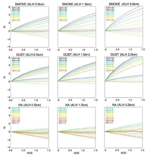
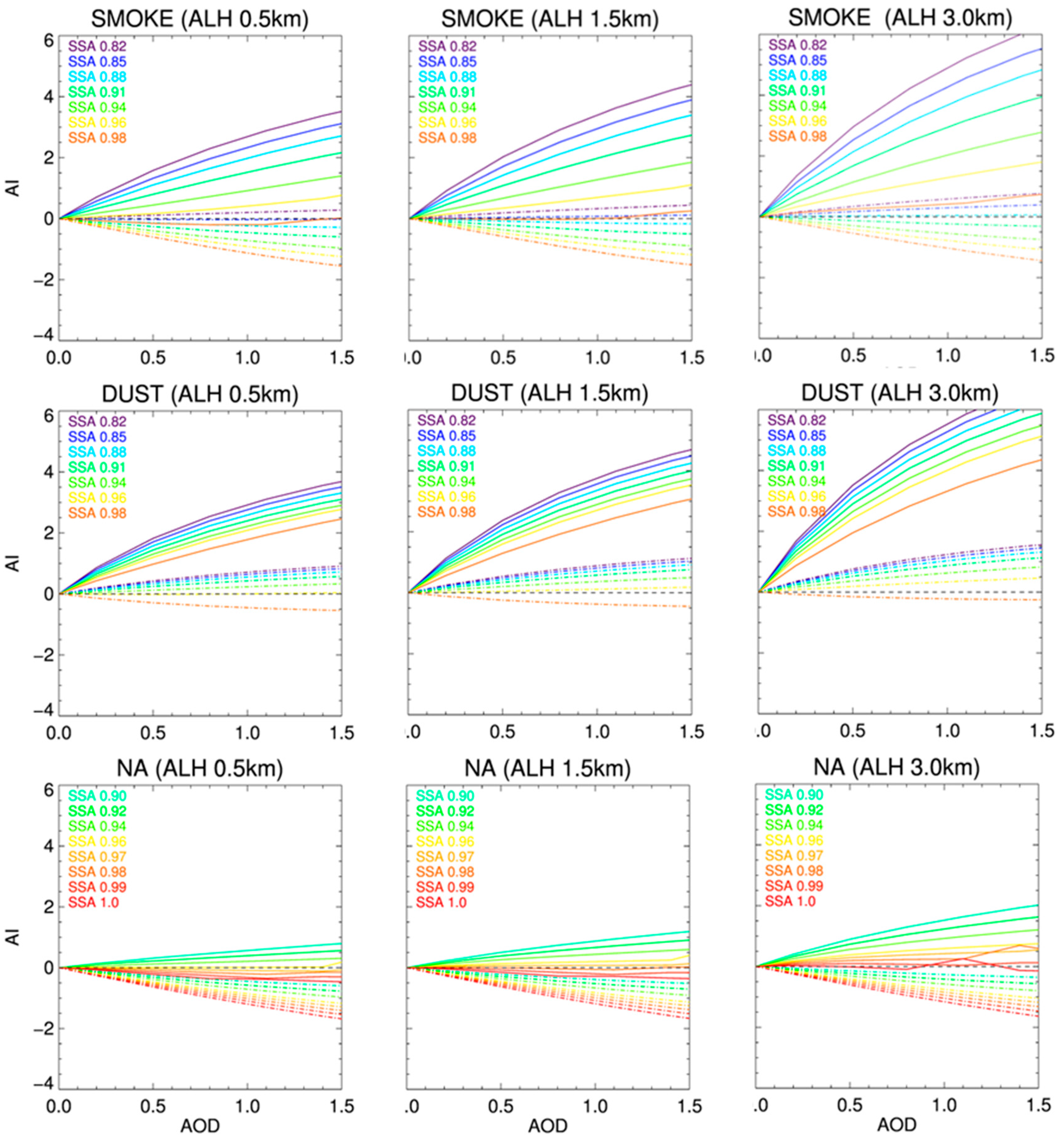
Figure 1 shows the simulated results of UVAI and SAI with respect to aerosol types, aerosol layer height (ALH), AOD, and single scattering albedo (SSA) using VLIDORT. Atmospheric radiative quantities of number-weighted aerosol particle size distributions and refractive indexes are summarized in Table 1. rm1 and rm2 denote a fine and coarse mode radius, respectively, and σm1 and σm2 denote fine and coarse mode variance, respectively. The fraction of m1 refers to the ratio of the fine mode number to the total number distribution. The last column in Table 1 presents the assumed real refractive index. Each aerosol type is divided by seven or eight aerosol models of varying SSA, for a total of 22 microphysical models (Table 2).
Aerosol optical properties, such as particle size distributions and their refractive indices, are obtained from AERONET 46 sites lv.2 Inversion data within 100°E–150°E, 20°N–50°N [9,28]. These data provide the most realistic aerosol information for East Asia. The aerosol types (fine-absorbing particles or smoke, dust, and NA) are classified, based on the method proposed by Lee et al. [27], using 550 nm FMF and 440 nm SSA. Smoke and NA aerosol types showed fine-mode dominant volume size distribution, while dust aerosol showed course-mode dominant volume size distribution, and their volume size distributions are converted to number-weighted particle size distributions, as shown in Table 1. The UV wavelength spectral dependence of the imaginary refractive index of aerosol models is assumed from AERONET 440 nm measurements with a constant value of the absorption angstrom exponent (AAE) [2]. The highest spectral dependence of the imaginary refractive index is assumed for dust aerosols, while almost no spectral dependence of the imaginary refractive index is assumed for smoke aerosols. In VLIDORT, all aerosol models are considered as spherical particles, including dust aerosol models (see Appendix A). Table 2 summarizes the input parameters for the VLIDORT calculation used to simulate UVAI and SAI. The aerosol profiles are assumed to have a Gaussian distribution, with a full width at a half maximum (FWHM) of 1 km, and are set to be located between 0.1 and 10 km.
Figure 1 shows the UVAI (for 354 and 388 nm) and the SAI (for 388 nm) calculated using Equations (1) and (2), respectively. Although the sensitivity analysis examines changes for various input parameters, a set of fixed baseline values was used, including reflectivity (0.05), the Solar Zenith Angle (SZA) (36°), the Relative Azimuth Angle (RAA) (150°), the Viewing Zenith Angle (VZA) (38°), and surface elevation (0 km). The simulation results show that both UVAI and SAI have a sensitivity to SSA that increases for highly absorbing cases. As the aerosol layer height increases from 0.5 to 3.0 km, the path between the aerosol and the TOA becomes shorter, meaning that both AI signals increase. When considering the different aerosol types, dust AI is more sensitive to aerosol absorption because dust is known to have the highest spectral dependence of the imaginary refractive index in UV [29,30]. In Figure 1, the weakly absorbing aerosols of smoke and dust AI at lower altitudes cannot be distinguished from NA AI [8]. For brighter surfaces and higher terrain pressures (not shown), simulated UVAI and SAI seem to have a high signal sensitivity with aerosol loading. Although SAI is sensitive with respect to SSA, SAI at lower altitudes shows small and negative values, even for smoke and dust aerosols, when compared with UVAI, thus showing a limitation of the model simulations.
To overcome these problems for real measurements (Section 4), an investigation of the empirical SAI was performed to find the best background AI. Additionally, we verified the sensitivity of SAI with respect to SSA using six SAI empirical models.
4. Results
The present study area (Figure 2) covers the Korean Peninsula and the surrounding area in northeast Asia, including Korea, Taiwan, China, and Japan. This region experiences severe dust storms every spring and severe pollution in winter, causing high UVAI during these periods. A single path of OMI lv.2 UVAI (354 and 388 nm) data was projected for all OMI data crossing the study area during a single day. This day was marked by a severe dust storm to the northwest of the Korean Peninsula and highly absorptive aerosols with a UVAI value of >1.5. A sun-glint area near the east coast of China was removed because this area has a brighter surface than other ocean surface areas.
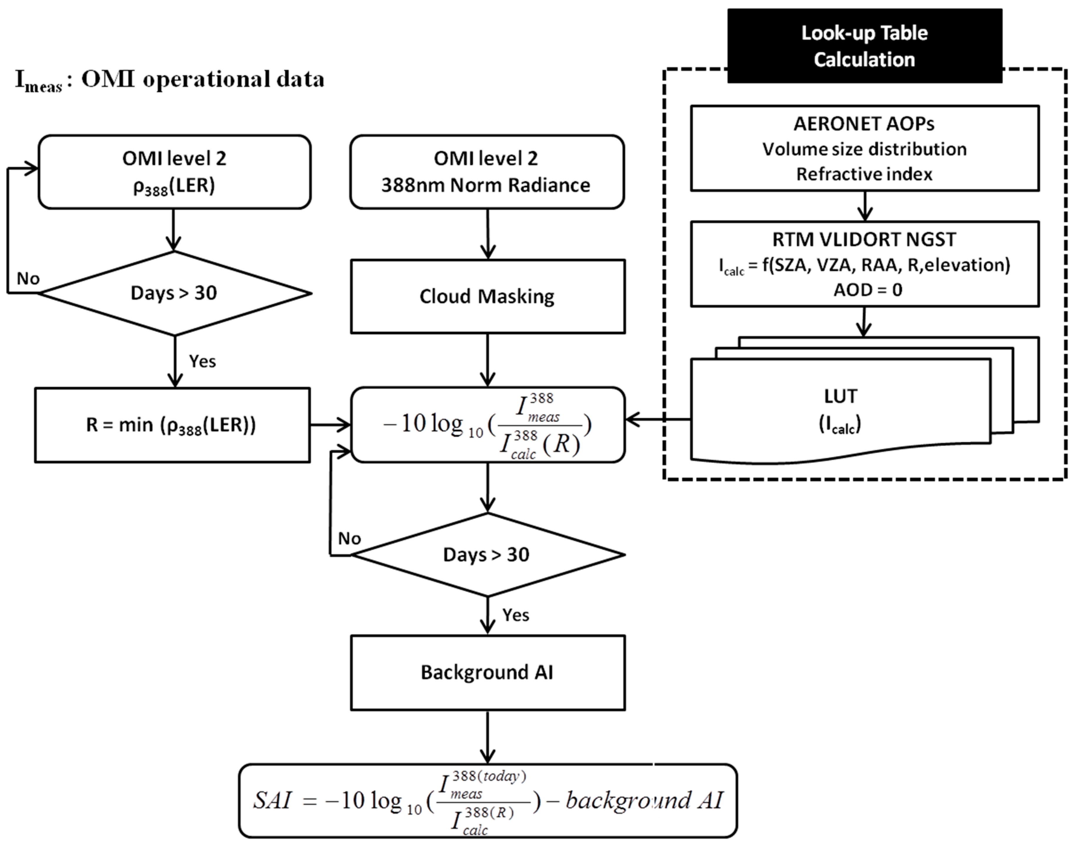
A flowchart of the SAI retrieval algorithm is presented in Figure 3. First, a surface reflectance (R) was produced for a 0.5° × 0.5° grid resolution by directly using the previous 30-day minimum OMI LER (lv.2) data, referred to as the minimum reflectance method. This method assumes at least one clear-sky day among the previous 30 days for a given pixel [31,32]. If the period exceeds 30 days, the surface reflectance could be contaminated by other factors, such as changes in vegetation cover. Secondly, a pre-calculated lookup table (LUT) was used to calculate . The LUT was constructed using a forward model, VLIDORT, to calculate the Rayleigh scattered radiance from the minimum reflectance. The input parameters used to construct the LUT are summarized in Table 3. After calculating for a clear sky area, was calculated from the OMI measurement data to allow the aerosol signals to be separated. The 30-day minimum values of in a 0.5° × 0.5° grid resolution were then defined as background AI. To avoid cloud contamination and uncertainties in radiometric calibration, OMI lv.2 normalized radiance data with a quality flag of zero, which indicates minimum cloud presence [17], are used. Finally, SAI is obtained from Equation (2) by subtracting the background AI from the aerosol signal. In the next section, to identify the best background AI, frequency distributions are used to evaluate detailed empirical background AI models.
4.1. Inter-Comparisons of SAI Obtained from Empirical Models
To derive the best background AI, SAI sensitivity with respect to SSA for six empirical models was analyzed. OMI lv.2 data for spring 2006 were selected for calculating several empirical models of SAI, the minimum reflectance, and background AI. The 2006 data were selected for this case study to avoid the row anomaly problem of OMI. The results for two days marked by severe dust storms and high UVAI are presented in Table 4. A particulate matter (PM) concentration of 2298 µg/m3 was observed over the Korean Peninsula on 8 April 2006, and 50~400 µg/m3 was recorded on 23 April 2006.
To consistently assess the SAI sensitivity with respect to SSA, only AOD values greater than 0.5 and UVAI values greater than 0.5 were selected, to ensure the retrieval accuracy of the SAI algorithm. The calculated slope of regression and the correlation coefficient (R) are presented in Table 4. Six empirical SAI models (M0 to M5) are categorized in Table 4. For empirical model M0, the background AI is zero. For models M1 to M5, each background AI refers to a selected value of M0 among 30 days in the following ways: non-cloud-screened minimum composite (M0-minM0), cloud-screened minimum composite, cloud-screened mean composite (M0-meanM0), cloud-screened median composite (M0-medianM0), and the absolute value of the cloud-screened minimum composite (M0-min(absM0)), respectively.
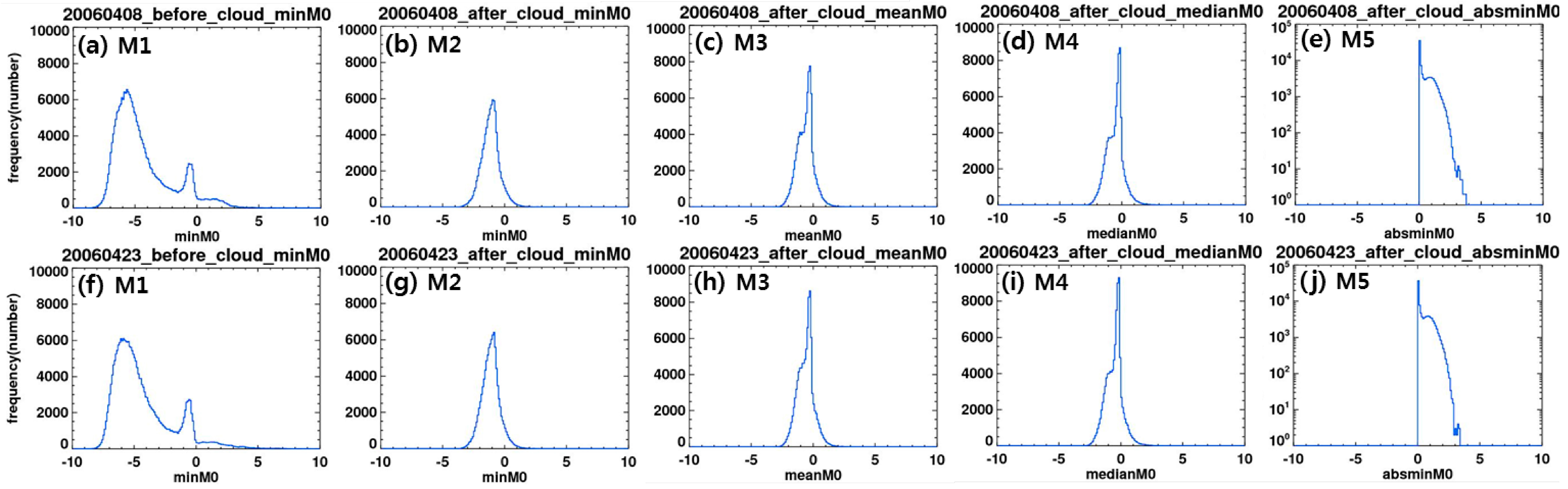
Figure 4 shows the frequency distribution of background AI for each empirical model (M1 to M5) for two days, using the 388 nm channel of OMI. Background AIs are enumerated in the same order as the bold characters in Table 4. Among the five background AIs, the minimum composite of the cloud-screened M0 values (Figure 4b,g) is closest to a Gaussian distribution and is evenly distributed, indicating that the background AIs are randomly selected.
Figure 5 shows scatter plots of SAI with respect to SSA for 8 April 2006. OMI lv.2 data are used to determine the aerosol type, and most of the scenes are classified as smoke. Six empirical SAI models, from M0 to M6, show a proportional relationship with SSA and exhibit a negative slope. However, M2 shows the best proportional relationship with respect to SSA, with a root mean square error (RMSE) of 0.723, except for NA aerosols, which were assumed to have an SSA equal to one [17]. Therefore, from Table 4 and Figure 4 and Figure 5, M2 was chosen as the best SAI model, given the correlation coefficient of scatter plot data, distribution of scatter plot data with the RMSE value, and the Gaussian distribution of background AI.
In a physical sense, the background AI of M2 is a composite result of the strongest scattering signal among the previous 30 days. Therefore, subtracting minM0 will make the SAI absorbing aerosol signals more dominant. M2 is sufficient for discerning the aerosol absorption, as described in Section 4.2 and Section 4.3. However, empirically selecting the background AI could limit the performance of the current algorithm because the background AI may differ in different regions.
For M1, compositing minM0 without cloud screening resulted in a weaker correlation because it contains a thick cloud signal. The M1 background AI shows a large negative value compared with the non-cloud areas (not shown).
The background AI signal may be changed with respect to different composite periods, since surface vegetation changes throughout the year. To examine the influence of surface reflectance, we also tried to composite more than 30 days of background AI (e.g., 40, 50, and 60 days), but the composited value of background AI did not show a significant change to the 30-day composite periods. Therefore, only M2 (M0-minM0, after cloud screening) was used in our algorithm.
4.2. Performance of SAI Obtained from OMI (Including Validation with UVAI)
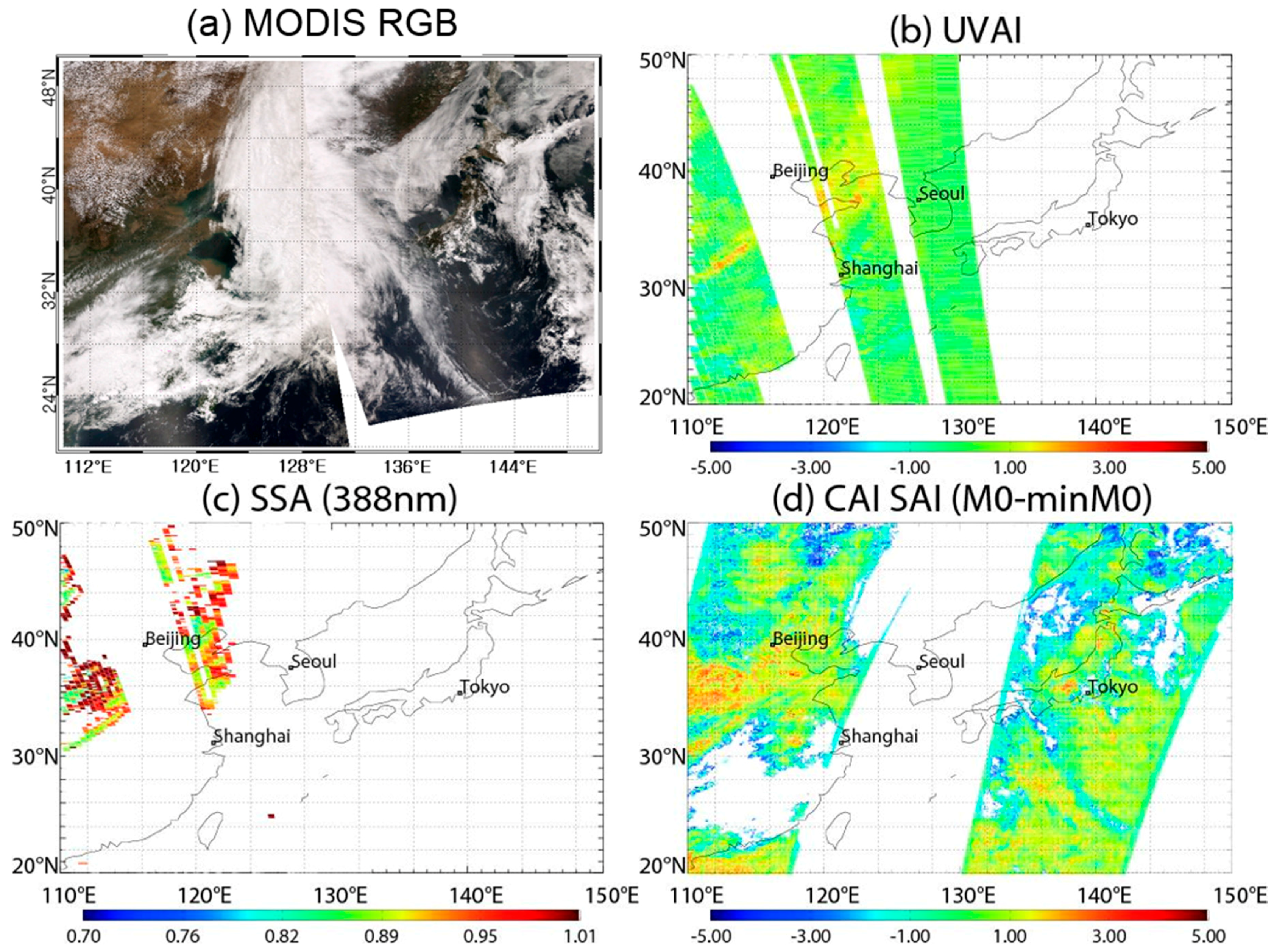
Figure 6 shows a large Asian dust event that occurred on 23 April 2006, as shown in MODIS true color images and also OMI UVAI, OMI SSA, and SAI. On this day, a thick absorbing aerosol layer can be observed over northeast China, extending to western Korea, as shown in Figure 6a using a MODIS true color (650, 555, 465 nm as RGB respectively) image. AOD was higher than 1.5, indicating thick optical aerosol layers. The UVAI values higher than 2.5 from OMI (Figure 6b) show strong UV absorption for the dust layer located over the Yellow Sea. MODIS and OMI have 8-min time differences onboard the NASA’s A-train satellite. The SAI retrieval (Figure 6d) shows strong absorbing aerosols, where the OMI SSA for the 388 nm channel (Figure 6c) ranges from 0.82 to 0.90, and the UVAI ranges from 0.7 to 2.5, corresponding to the dust-laden area and over the Gobi Desert, as inferred from the MODIS RGB image.
The OMI user guide has mentioned that ocean surface reflectance shows distinct angular and spectral variations compared to land, due to spectral varying scattering from the water, often called water-leaving radiances (WLR), chlorophyll, sediments, and other types of suspended matter which decrease the WLR. This WLR causes the main error of aerosol retrieval over the ocean. Since this short term variability is not taken into account in the current version of the algorithm, OMI SSA has been retrieved over an area where the UVAI are over 0.8. For the same reason, SAI over the north-east part of the Korean peninsula has been screened out. The SAI values are proportional to an SSA value of 388 nm over western Korea, showing a linear relationship.
To qualitatively evaluate the statistical results of the developed SAI algorithm with UVAI, the agreement and false detection rate are calculated by using the following equations:
where NUVAI&SAI denotes the number of absorbing aerosol pixels defined by both the OMI UVAI and SAI algorithms, simultaneously. NUVAI and NSAI denote the number of absorbing aerosol pixels detected by the OMI UVAI algorithm and the SAI algorithm, respectively (Park et al. [33]).
Figure 7 shows the agreement and false detection of absorbing aerosol results between the OMI UVAI algorithm and the OMI SAI algorithm for 8 April 2006 (Figure 7a–c) and 23 April 2006 (Figure 7d–i), respectively. Because SSA is assumed to be one in the OMI algorithm for an NA aerosol scene, the pixels with SSA values lower than 1.0 are used for the inter-comparison, to ensure the retrieval accuracy of the SAI algorithms. The results are only compared for areas where OMI SSA exists. Since OMI UVAI can be used to detect the absorbing aerosol region with UVAI values higher than 0.7 [17], UVAI values of 0.5, 0.7, and 1.0 from OMI are used as reference values. To calculate the SAI absorbing aerosol threshold, values of −0.5 to 1.5 are used, as shown on the x-axis in Figure 7. Given that the SAI values are generally distributed between −1 and 3, values from −1 to −0.5 and from 1.5 to 3 were excluded, to avoid any statistical errors arising from sampling small numbers of pixels.
The agreement between the absorbing aerosols inferred from the UVAI and the SAI algorithms decreases significantly beyond a threshold value of 0.5 for SAI (Figure 7). Conversely, the false detection rate is almost invariable over all of the SAI threshold values (x-axis ranges), which indicates that SAI values higher than 0.5 qualitatively correspond to a UVAI value larger than 0.7, because 80% of the SAI are also detected with UVAI. This tendency is clearer for highly absorbing cases (SSA < 0.90). Note that although the agreement area falls rapidly for values above 0.5 because of a small threshold, the SAI false detection rate remains stable, which in turn means that the number of false detections in SAI is small. Therefore, 90% of the SAI is also detected with UVAI. For a strongly absorbing aerosol case at 0458 UTC on 23 April 2006, the SSA ranged between 0.82 and 0.90, and the false detection rate of SAI was consistently below 0.1 for the UVAI threshold of 0.7.
No significant changes were observed with AOD criteria higher than 0.5. This result indicates that the SAI absorbing aerosol threshold primarily depends on SSA. The results show that although the SAI pattern is similar to SSA and the SAI value over 0.5 matches well with a UVAI threshold of 0.7, the agreement and false detection test with OMI shows a consistent and meaningful correlation. The SAI value of 0.5 corresponds to a UVAI value of 0.7. As a result, the current SAI algorithm correctly defines a high percentage of the absorbing aerosol pixels.
4.3. Performance of SAI Obtained from TANSO-CAI (Including Validation with UVAI)
The SAI algorithm was applied to the TANSO-CAI instrument to verify the feasibility of aerosol absorption detection using the SAI algorithm with a single broadband UV channel. The minimum LER values from 30 days were used for the composite surface reflectance and background AI. However, since band 1 of TANSO-CAI has a narrow swath of 1000 km and a three-day recursion period, the same paths of 30-day data among 90 days were used. Dark and invariable UV surface reflectance in the 90-day composite make it possible to employ this approach without any significant errors. The advantage of applying the SAI algorithm to TANSO-CAI is that it can detect the absorbing aerosols with a 500 m resolution. To reduce the calculation time, all TANSO-CAI data were re-gridded with a 0.1° resolution. To select the TANSO-CAI case-study days, the time difference between TANSO-CAI and OMI within 10 min was calculated.
The absorbing aerosol cases for two days, 17 March and 25 April 2012, were selected to test TANSO-CAI SAI with OMI UVAI (Figure 8 and Figure 9, respectively). On 17 March 2006, a thin absorbing aerosol layer was observed over the western Korean Peninsula and eastern China using MODIS RGB (Figure 8a). The OMI UVAI (Figure 8b) showed values higher than 1.6, representing moderate UV absorption over the dust layer located over eastern China. The white area in the middle of the UVAI (Figure 8b) represents the row anomaly pixels of OMI. The SAI algorithm from TANSO-CAI (Figure 8d) successfully detects the moderate absorbing aerosol layers with a SAI value above 2.0. As inferred from previous results from OMI, the SAI algorithm detects OMI SSA (Figure 8c) over eastern China with a linear relationship. For this day, the moderate absorbing aerosol layer showed AOD values higher than 1.0.
A weakly absorbing aerosol case is shown in Figure 9, for 25 April 2006. Weakly absorbing aerosols are detected in the MODIS RGB image over the northwestern Korean Peninsula (Figure 9a). Figure 9d shows the SAI algorithm results of TANSO-CAI for this case, which shows weakly absorbing aerosols where OMI SSA (Figure 9c) ranges from 0.88 to 0.91 and UVAI (Figure 9b) ranges from 0.8 to 1.0, over the same absorbing area as that inferred from the MODIS RGB image. At the same time, the AOD values exceeded 1.0 over the investigated region. Unfortunately, because of the OMI row anomaly problem, some of the scenes over China are not shown, although TANSO-CAI SAI results are given. For TANSO-CAI SAI, the blue-colored SAI pixels show the cloud edge area and the edge problem related to TANSO-CAI band 1 [23].
The agreement and false detection are calculated for TANSO-CAI SAI and OMI UVAI data, to evaluate the TANSO-CAI SAI algorithm. However, to reduce the error that arises from the time difference, only TANSO-CAI and OMI data within 10 min of each other are compared, whereas all TANSO-CAI data are plotted in Figure 8 and Figure 9. In addition, to reduce the statistical error originating from inaccurate SSA, only OMI data with an SSA less than 1.0 were used in the comparison. To spatially compare OMI UVAI and TANSO-CAI, both datasets, as well as SSA from OMI, were re-gridded to a 0.5° grid resolution.
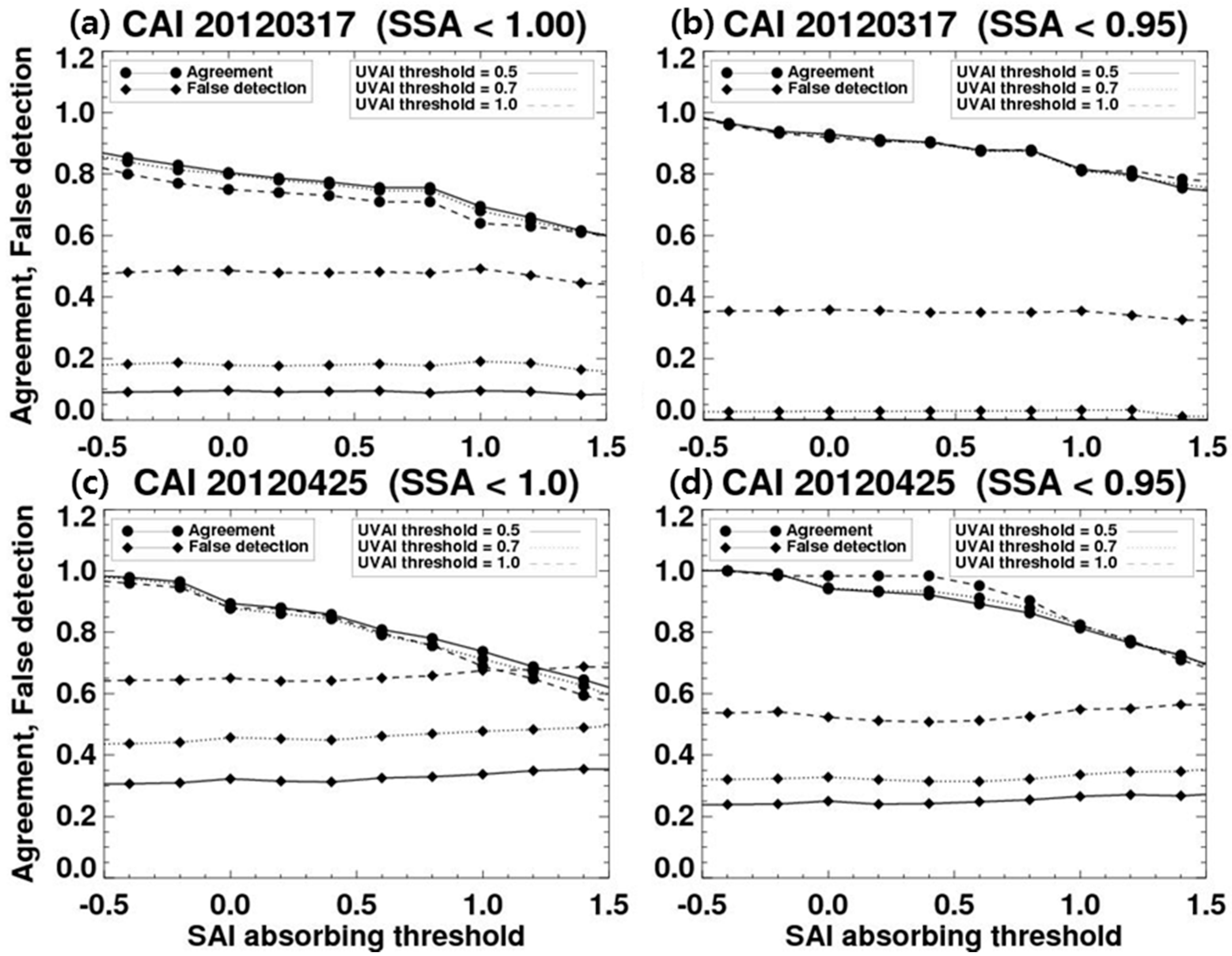
Figure 10 shows the agreement and false detection results for the two TANSO-CAI cases. These two cases of TANSO-CAI SAI, on 17 March 2012 (Figure 10a,b) and 25 April 2012 (Figure 10c,d), were compared with OMI UVAI. The colored numbers (0.5, 0.7, and 1.0) in Figure 10 indicate the OMI UVAI threshold. The x-axis denotes TANSO-CAI SAIs, which generally have values between –1 and 3. TANSO-CAI SAI absorbing aerosol threshold values are tested from–0.5 to 2.0, at 0.2 intervals. The case on 17 March 2012 (Figure 10a,b) is a moderate absorbing aerosol, while 25 April 2012 (Figure 10c,d) is a weakly absorbing aerosol. In Figure 10, the agreement consistently decreases with an increasing TANSO-CAI SAI absorbing aerosol threshold. In contrast, the false detection rate with UVAI values of 0.7 is almost invariable over all thresholds, especially with an error of <0.1 in Figure 10b. This indicates that >80% of the TANSO-CAI SAI values qualitatively correspond to UVAI values of >0.7. However, in Figure 10a,c,d, the false detection rate values are slightly higher than those in Figure 7. This difference could be caused by the 10-min time difference between TANSO-CAI and OMI, or the signal contamination during the re-gridding of OMI and TANSO-CAI. Alternatively, it may have arisen because the minimum reflectance of TANSO-CAI was different to that of OMI, or because of a TANSO-CAI calibration issue. Furthermore, the difference could be related to Figure 10a,c,d not including a strong absorbing aerosol case. For highly absorbing cases (SSA < 0.90), the false detection rate decreased significantly, indicating that the error in the results originates from a low aerosol absorption signal.
5. Discussion
UVAI is a practical parameter for assessing aerosol absorption and type, with a principle of measuring the spectral contrast in the UV range. Currently, UVAI is provided from OMI with a 13 × 24 km2 nadir resolution. In contrast, an instrument such as TANSO-CAI cannot provide UVAI, thus demonstrating a limitation in providing information on the absorbing aerosol type, which leads to errors in AOD, CO2, and relevant products, although the instrument has a higher spatial resolution of 500 m. A single UV channel on TANSO-CAI makes this challenging. To address this challenge, an SAI algorithm was developed.
The results of SAI from the OMI hyperspectral band and the TANSO-CAI broadband are compared with the OMI UVAI. By applying the SAI algorithm to OMI and TANSO-CAI, we found that the false detection rate of the results is consistently low for both instruments. This suggests that the current SAI rarely detects non-absorbing aerosols. In other words, the TANSO-CAI SAI results are consistent with the OMI SAI results. This also implies that the SAI absorbing aerosol threshold primarily depends on SSA. However, it is difficult to decide on the exact threshold of SAI, because SAI could detect absorbing aerosol pixels with <20% error, at least for moderate absorbing aerosol cases. Error ranges become even smaller for highly absorbing aerosol cases.
The effectiveness of the SAI directly depends on the proper selection of the background AI. To use SAI in the operational algorithm in stable conditions, the following methods are recommended for a further investigation in the future.
First, the empirical parameter background AI should be investigated seasonally and globally. In this study, the background AIs of M2 for a 30-day window composite was similar to those for 40-day, 50-day, and 60-day window composite durations. However, seasonally and globally, a 30-day window composite could be affected by cloud [32]. Similarly, Kim et al. [31] have shown improved AOD results after proper background optical depth correction.
Second, a cloud screening algorithm should be strictly applied. If cloud has not been strictly screened out, background AI could have a large negative value, and this would affect the SAI. In this study, a simple LER cut method is applied as a cloud screening algorithm to retrieve CAI SAI. Therefore, CAI SAI is possibly affected by cloud.
Moreover, the error due to using spherical model particles for dust aerosols should be re-considered. In this study, UVAI and SAI are simulated with spherical models, including dust aerosols. Since the principle of the UVAI is to measure the spectral contrast in the UV range, UVAI might be less affected by phase function differences between spherical particles and spheroid particles [10,26]. However, SAI simulation results may be affected by phase function differences between spherical particles and spheroid particles [34,35]. Therefore, in a further study, it is recommended that dust aerosols are calculated with a non-spherical database [26,36].
To our knowledge, this is the first time that a single UV channel has been used for an absorbing aerosols detection algorithm. The algorithm has the potential to be used with other sensors that have just a single UV channel. In addition, the absorbing aerosol detection product can be used for the quantitative retrieval of aerosol optical thickness, by forcing the algorithm to select a lookup table generated for absorbing aerosol models.
6. Conclusions
We developed an SAI algorithm using the OMI hyperspectral band and the TANSO-CAI broadband, and compared it with OMI UVAI to detect aerosol absorption from UV-constrained satellites. The SAI is physically defined as a measure of the degree to which the absorbing aerosols differ from purely molecular atmosphere conditions. Radiative transfer calculations for representative aerosols were assessed to calculate the sensitivity of UVAI and SAI at the TOA, before applying the SAI algorithm. An empirical model for adopting the best background AI was developed and analyzed.
SAI showed a proportional relationship with SSA, which implies that SAI has an aerosol absorption signal. In addition, an agreement and false detection test with UVAI was developed, which showed that the false detection signal did not change with respect to the UVAI absorbing threshold value. This means that SAI rarely detects non-absorbing signals. The results were not dependent on the type of satellite instrument.
The advantage of the SAI algorithm is its adaptability to other satellite platforms that only have a single UV channel. A Geostationary Ocean Color Imager(GOCI)-2 is another instrument with a single UV channel, to be launched in 2019. This opens up the possibility of absorbing aerosol detection for the next generation of satellite sensors, as well as past satellite data. However, the absorption threshold of SAI is dependent on the instrument, which limits this research. Therefore, future work is needed to identify a global threshold from several absorbing cases, to extend climate research. This study is meaningful for the detection of aerosol absorption using instruments with a single UV channel. Future work will involve the adaptation of the SAI-based algorithm to several satellite instruments that cover a large area for a long duration.
Acknowledgments
We would like to thank the AERONET network and the principal investigators, as well as their staff, for establishing and maintaining the AERONET sites used in this work. This subject is supported by Korea Ministry of Environment(MOE) as "Public Technology Program based on Environmental Policy(RE201702180)". This research was supported by the “Development of the integrated data processing system for GOCI-II” funded by the Ministry of Ocean and Fisheries, Korea. This research was partially supported by the Brain Korea 21 Plus (S. Go and J. Kim).
Author Contributions
M.K. and J.K. conceived and designed the experiments; S.G., M.K. and W.J. performed the experiments; S.P. and M.C. analyzed the data; W.J. and S.P. contributed reagents/materials/analysis tools; S.G. and J.K. wrote the paper.
Conflicts of Interest
The authors declare no conflict of interest.
Appendix A
Use of Spherical Particle Approximation in Mineral Dust Aerosols
Dust is known to be comprised of spheroid particles, so it should be simulated with non-sphericity consideration using a T-matrix code for e.g., with Dubovik data [26] or a Ping Yang’s database [36]. By Mishchenko et al. [37], it is known that the non-sphericity of desert dust particles can cause scattering properties significantly different from those predicted by the standard Mie theory, especially in the scattering angle range 100-180°. The importance of dust particle shape in radiance and flux simulations has also been pointed out by Kahnert and Kylling [34] and Yi et al. [35]. Kahnert and Kylling [34] pointed out that spherical assumed dust at 550 nm can cause errors in the diffuse spectral radiance between −16% and 115% at the top of the atmosphere (TOA), and could have an uncertainty in the extinction optical depth τ between 0.5τ and 2τ at the TOA. Yi et al. [35] simulated the uncertainties from the particle shape and refractive index with the Ping Yang database, and pointed out that the particle shape effect is found to be related to the dust optical depth and the surface albedo can be an important uncertainty source in radiative transfer simulation. Even though near-UV measurement is insensitive to aerosol phase function effects, as discussed by Torres et al. [10], the research done by Gasso et al. [38] showed that the dust LUT applied by the T-matrix code resulted in an increasing retrieval of AOD. However, a non-spherical model did not affect to SSA retrieved results, as noted by Kroktov et al. [39] and Dubovik et al. [26].
The error related to dust spherical particle approximation is mainly due to the misrepresentation of the aerosol phase function by the spheres, as mentioned by Kahnert and Kylling [34]. Dubovik et al. [26] presented the simulation results of the dust phase function with spheroids and a spherical aerosol model at 440 nm, 500 nm, 670 nm, 870 nm, and 1020 nm. When it comes to retrieving AOD, the AOD difference between spheroids and a sphere originates from the difference in the phase function of the spheroid and spherical model at the same wavelength. However, when it comes to retrieving UVAI, the only difference is the measurement wavelength, and the assumed phase function is the same. Therefore, we expect that the UVAI results between spheroids and the spherical model might not exhibit a big difference.
Moreover, Torres et al. [10] showed that, in the 320–400 nm range, the use of spherical particle approximation to retrieve aerosol products produces smaller errors than a similar estimate in the visible bands, because of the larger multiple-scattering contribution to the total backscattered intensity in the near UV. Furthermore, Van de Hulst. [40] said that the effect of particle shape on the scattering properties of non-spherical particles becomes weaker when increasing the imaginary component of the refractive index. Since the desert dust imaginary refractive index in the UV is almost an order of magnitude larger than at 630 nm, the effect on non-sphericity on the phase function may also be less important in the UV than in the visible spectrum.
References
- Myhre, G.; Berglen, T.; Johnsrud, M.; Hoyle, C.; Berntsen, T.; Christopher, S.; Fahey, D.; Isaksen, I.S.; Jones, T.; Kahn, R. Modelled radiative forcing of the direct aerosol effect with multi-observation evaluation. Atmos. Chem. Phys. 2009, 9, 1365–1392. [Google Scholar] [CrossRef]
- Russell, P.; Bergstrom, R.; Shinozuka, Y.; Clarke, A.; DeCarlo, P.; Jimenez, J.; Livingston, J.; Redemann, J.; Dubovik, O.; Strawa, A. Absorption angstrom exponent in aeronet and related data as an indicator of aerosol composition. Atmos. Chem. Phys. 2010, 10, 1155–1169. [Google Scholar] [CrossRef]
- Solomon, S. Climate Change 2007—The Physical Science Basis: Working Group I Contribution to the Fourth Assessment Report of the IPCC; Cambridge University Press: Cambridge, UK, 2007; Volume 4. [Google Scholar]
- Higurashi, A.; Nakajima, T. Detection of aerosol types over the east china sea near japan from four-channel satellite data. Geophys. Res. Lett. 2002, 29, 17:1–17:4. [Google Scholar] [CrossRef]
- Kim, J.; Lee, J.; Lee, H.C.; Higurashi, A.; Takemura, T.; Song, C.H. Consistency of the aerosol type classification from satellite remote sensing during the atmospheric brown cloud–East Asia regional experiment campaign. J. Geophys. Res. Atmos. 2007, 112. [Google Scholar] [CrossRef]
- Torres, O.; Tanskanen, A.; Veihelmann, B.; Ahn, C.; Braak, R.; Bhartia, P.K.; Veefkind, P.; Levelt, P. Aerosols and surface uv products from ozone monitoring instrument observations: An overview. J. Geophys. Res. Atmos. 2007, 112. [Google Scholar] [CrossRef]
- Li, Q.; Li, C.; Mao, J. Evaluation of atmospheric aerosol optical depth products at ultraviolet bands derived from MODIS products. Aerosol Sci. Technol. 2012, 46, 1025–1034. [Google Scholar] [CrossRef]
- Herman, J.; Bhartia, P.; Torres, O.; Hsu, C.; Seftor, C.; Celarier, E. Global distribution of UV-absorbing aerosols from nimbus 7/toms data. J. Geophys. Res. Atmos. 1997, 102, 16911–16922. [Google Scholar] [CrossRef]
- Dubovik, O.; King, M.D. A flexible inversion algorithm for retrieval of aerosol optical properties from sun and sky radiance measurements. J. Geophys. Res. 2000, 105, 20673–20696. [Google Scholar] [CrossRef]
- Torres, O.; Bhartia, P.; Herman, J.; Ahmad, Z.; Gleason, J. Derivation of aerosol properties from satellite measurements of backscattered ultraviolet radiation: Theoretical basis. J. Geophys. Res. Atmos. 1998, 103, 17099–17110. [Google Scholar] [CrossRef]
- Higurashi, A.; Nakajima, T. Development of a two-channel aerosol retrieval algorithm on a global scale using noaa avhrr. J. Atmos. Sci. 1999, 56, 924–941. [Google Scholar] [CrossRef]
- Kaufman, Y.J.; Fraser, R.S.; Ferrare, R.A. Satellite measurements of large-scale air pollution: Methods. J. Geophys. Res. Atmos. 1990, 95, 9895–9909. [Google Scholar] [CrossRef]
- Jeong, M.J.; Li, Z. Quality, compatibility, and synergy analyses of global aerosol products derived from the advanced very high resolution radiometer and total ozone mapping spectrometer. J. Geophys. Res. Atmos. 2005, 110. [Google Scholar] [CrossRef]
- Jung, Y.; Kim, J.; Kim, W.; Boesch, H.; Lee, H.; Cho, C.; Goo, T.-Y. Impact of aerosol property on the accuracy of a CO2 retrieval algorithm from satellite remote sensing. Remote Sens. 2016, 8, 322. [Google Scholar] [CrossRef]
- Dobber, M.; Kleipool, Q.; Dirksen, R.; Levelt, P.; Jaross, G.; Taylor, S.; Kelly, T.; Flynn, L.; Leppelmeier, G.; Rozemeijer, N. Validation of ozone monitoring instrument level 1b data products. J. Geophys. Res. Atmos. 2008, 113. [Google Scholar] [CrossRef]
- Levelt, P.F.; Van den Oord, G.H.; Dobber, M.R.; Malkki, A.; Visser, H.; De Vries, J.; Stammes, P.; Lundell, J.O.; Saari, H. The ozone monitoring instrument. IEEE Trans. Geosci. Remote Sens. 2006, 44, 1093–1101. [Google Scholar] [CrossRef]
- Torres, O.; Ahn, C.; Chen, Z. Improvements to the OMI near-UV aerosol algorithm using A-train CALIOP and AIRS observations. Atmos. Meas. Tech. 2013, 6, 3257–3270. [Google Scholar] [CrossRef]
- Jethva, H.; Torres, O.; Ahn, C. Global assessment of omi aerosol single-scattering albedo using ground-based aeronet inversion. J. Geophys. Res. Atmos. 2014, 119, 9020–9040. [Google Scholar] [CrossRef]
- Yokota, T.; Yoshida, Y.; Eguchi, N.; Ota, Y.; Tanaka, T.; Watanabe, H.; Maksyutov, S. Global concentrations of CO2 and CH4 retrieved from gosat: First preliminary results. Sola 2009, 5, 160–163. [Google Scholar] [CrossRef]
- Kuze, A.; Suto, H.; Nakajima, M.; Hamazaki, T. Thermal and near infrared sensor for carbon observation fourier-transform spectrometer on the greenhouse gases observing satellite for greenhouse gases monitoring. Appl. Opt. 2009, 48, 6716–6733. [Google Scholar] [CrossRef] [PubMed]
- Yoshida, Y.; Ota, Y.; Eguchi, N.; Kikuchi, N.; Nobuta, K.; Tran, H.; Morino, I.; Yokota, T. Retrieval algorithm for CO2 and CH4 column abundances from short-wavelength infrared spectral observations by the greenhouse gases observing satellite. Atmos. Meas. Tech. 2011, 4, 717–734. [Google Scholar] [CrossRef]
- Fukuda, S.; Nakajima, T.; Takenaka, H.; Higurashi, A.; Kikuchi, N.; Nakajima, T.Y.; Ishida, H. New approaches to removing cloud shadows and evaluating the 380 nm surface reflectance for improved aerosol optical thickness retrievals from the gosat/tanso-cloud and aerosol imager. J. Geophys. Res. Atmos. 2013, 118. [Google Scholar] [CrossRef]
- Kuze, A.; Suto, H.; Shiomi, K.; Urabe, T.; Nakajima, M.; Yoshida, J.; Kawashima, T.; Yamamoto, Y.; Kataoka, F.; Buijs, H. Level 1 algorithms for TANSO on GOSAT: Processing and on-orbit calibrations. Atmos. Meas. Tech. 2012, 5, 2447–2467. [Google Scholar] [CrossRef]
- Spurr, R. Lidort and vlidort: Linearized pseudo-spherical scalar and vector discrete ordinate radiative transfer models for use in remote sensing retrieval problems. In Light Scattering Reviews 3; Springer: Heidelberg, Germany, 2008; pp. 229–275. [Google Scholar]
- De Rooij, W.; Van der Stap, C. Expansion of Mie scattering matrices in generalized spherical functions. Astron. Astrophys. 1984, 131, 237–248. [Google Scholar]
- Dubovik, O.; Sinyuk, A.; Lapyonok, T.; Holben, B.N.; Mishchenko, M.; Yang, P.; Eck, T.F.; Volten, H.; Munoz, O.; Veihelmann, B. Application of spheroid models to account for aerosol particle nonsphericity in remote sensing of desert dust. J. Geophys. Res. Atmos. 2006, 111. [Google Scholar] [CrossRef]
- Lee, J.; Kim, J.; Song, C.; Kim, S.; Chun, Y.; Sohn, B.; Holben, B. Characteristics of aerosol types from aeronet sunphotometer measurements. Atmos. Environ. 2010, 44, 3110–3117. [Google Scholar] [CrossRef]
- Dubovik, O.; Holben, B.; Eck, T.F.; Smirnov, A.; Kaufman, Y.J.; King, M.D.; Tanré, D.; Slutsker, I. Variability of absorption and optical properties of key aerosol types observed in worldwide locations. J. Atmos. Sci. 2002, 59, 590–608. [Google Scholar] [CrossRef]
- Mok, J.; Krotkov, N.A.; Arola, A.; Torres, O.; Jethva, H.; Andrade, M.; Labow, G.; Eck, T.F.; Li, Z.; Dickerson, R.R. Impacts of brown carbon from biomass burning on surface uv and ozone photochemistry in the Amazon Basin. Sci. Rep. 2016, 6. [Google Scholar] [CrossRef] [PubMed]
- Wagner, R.; Ajtai, T.; Kandler, K.; Lieke, K.; Linke, C.; Müller, T.; Schnaiter, M.; Vragel, M. Complex refractive indices of Saharan dust samples at visible and near UV wavelengths: A laboratory study. Atmos. Chem. Phys. 2012, 12, 2491–2512. [Google Scholar] [CrossRef]
- Kim, M.; Kim, J.; Wong, M.S.; Yoon, J.; Lee, J.; Wu, D.; Chan, P.; Nichol, J.E.; Chung, C.-Y.; Ou, M.-L. Improvement of aerosol optical depth retrieval over Hong Kong from a geostationary meteorological satellite using critical reflectance with background optical depth correction. Remote Sens. Environ. 2014, 142, 176–187. [Google Scholar] [CrossRef]
- Lee, J.; Kim, J.; Song, C.H.; Ryu, J.-H.; Ahn, Y.-H.; Song, C. Algorithm for retrieval of aerosol optical properties over the ocean from the geostationary ocean color imager. Remote Sens. Environ. 2010, 114, 1077–1088. [Google Scholar] [CrossRef]
- Park, S.S.; Kim, J.; Lee, J.; Lee, S.; Kim, J.S.; Chang, L.S.; Ou, S. Combined dust detection algorithm by using MODIS infrared channels over East Asia. Remote Sens. Environ. 2014, 141, 24–39. [Google Scholar] [CrossRef]
- Kahnert, M.; Kylling, A. Radiance and flux simulations for mineral dust aerosols: Assessing the error due to using spherical or spheroidal model particles. J. Geophys. Res. Atmos. 2004, 109. [Google Scholar] [CrossRef]
- Yi, B.; Hsu, C.N.; Yang, P.; Tsay, S.-C. Radiative transfer simulation of dust-like aerosols: Uncertainties from particle shape and refractive index. J. Aerosol Sci. 2011, 42, 631–644. [Google Scholar] [CrossRef]
- Meng, Z.; Yang, P.; Kattawar, G.W.; Bi, L.; Liou, K.; Laszlo, I. Single-scattering properties of tri-axial ellipsoidal mineral dust aerosols: A database for application to radiative transfer calculations. J. Aerosol Sci. 2010, 41, 501–512. [Google Scholar] [CrossRef]
- Mishchenko, M.I.; Travis, L.D.; Kahn, R.A.; West, R.A. Modeling phase functions for dustlike tropospheric aerosols using a shape mixture of randomly oriented polydisperse spheroids. J. Geophys. Res. Atmos. 1997, 102, 16831–16847. [Google Scholar] [CrossRef]
- Gassó, S.; Torres, O. The role of cloud contamination, aerosol layer height and aerosol model in the assessment of the omi near-uv retrievals over the ocean. Atmos. Meas. Tech. 2016, 9, 3031–3052. [Google Scholar] [CrossRef]
- Krotkov, N.A.; Flittner, D.; Krueger, A.; Kostinski, A.; Riley, C.; Rose, W.; Torres, O. Effect of particle non-sphericity on satellite monitoring of drifting volcanic ash clouds. J. Quant. Spectrosc. Radiat. Transf. 1999, 63, 613–630. [Google Scholar] [CrossRef]
- Van de Hulst, H.C.; Twersky, V. Light scattering by small particles. Phys. Today 1957, 10, 28–30. [Google Scholar] [CrossRef]
Figure 1.
Comparison of model-simulated UVAI and SAI with respect to AOD, SSA, aerosol types, and aerosol layer height using VLIDORT. Solid lines indicate UVAI (354, 388 nm) and dashed lines indicate SAI (388 nm) using Equations (1) and (2). The aerosol’s SSA are indicated at top left. The surface albedo and terrain pressure are 0.05 and 1014 mb, respectively. The three aerosol types (smoke, dust, and NA) and their optical properties were obtained from AERONET lv.2 Inversion data using the aerosol classifying method of Lee et al. [27].

Figure 2.
A single path of OMI UVAI data is projected for all OMI data for the Korean Peninsula and surroundings (top). MODIS True Color image (bottom) with an 8 min time difference compared with OMI, showing a severe dust storm over the Korean Peninsula, which originated in north China. Highly absorbing aerosols within the dust storm were detected by OMI UVAI with values greater than 1.5.
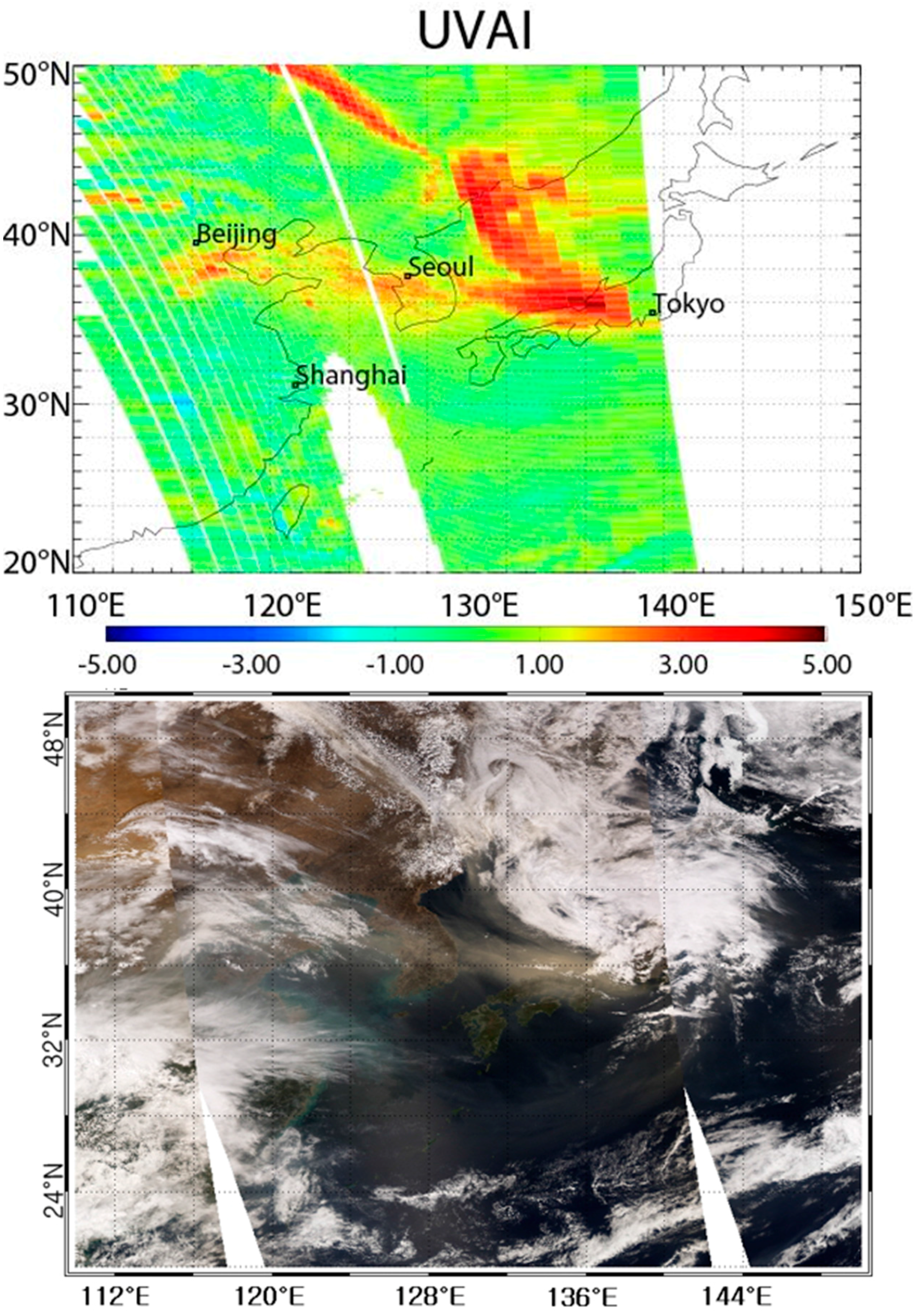
Figure 3.
Flowchart of the SAI retrieval algorithm using the 388 nm instrument channel of OMI. To avoid bias in the algorithms, measurement quality flags of zero, pixel quality flags of zero, and final algorithm flags of zero and one are used in the OMI lv.2 data.
Figure 3.
Flowchart of the SAI retrieval algorithm using the 388 nm instrument channel of OMI. To avoid bias in the algorithms, measurement quality flags of zero, pixel quality flags of zero, and final algorithm flags of zero and one are used in the OMI lv.2 data.

Figure 4.
(a–j) Frequency distribution of background AIs from Table 4. Upper panel shows results for 8 April 2006 and lower panel for 23 April 2006. From left to right, the frequency distributions show each background AI with cloud minimum M0 (a,f), without cloud minimum M0 (b,g), without cloud mean M0 (c,h), without cloud median M0 (d,i), and without cloud absolute minimum M0 (e,j). (e,j) plotted on a log scale on the y-axis. Among the five empirical background AI models, the minimum M0 (b), (g) shape is most likely to have a Gaussian distribution and is evenly distributed.

Figure 5.
Scatter plot of SAIs (388 nm) versus OMI lv.2 SSA for 8 April 2006. The empirical model of SAIs from (a) to (f) is the same as that listed in Table 4. These scatterplots use an AOD criterion of greater than 0.5 and a UVAI criterion of greater than 0.5 pixels. Among the five empirical SAI models, the M2 (c) has the smallest RMSE value.
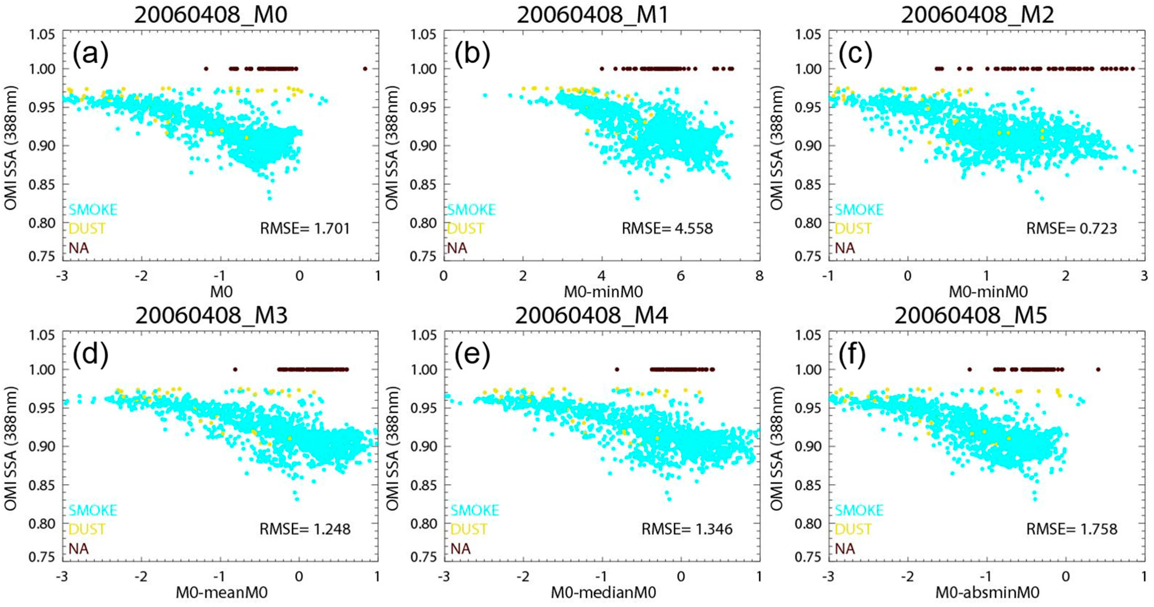
Figure 6.
(a) MODIS RGB has an 8-min time difference compared with OMI. (b) OMI UVAI, (c) OMI SSA, and (d) calculated SAIs over the Korean Peninsula, comparing UTC 0319 and UTC 0458 on 23 April 2006. PM10 concentrations were between 50 and 400 µg/m3 on this day.
Figure 6.
(a) MODIS RGB has an 8-min time difference compared with OMI. (b) OMI UVAI, (c) OMI SSA, and (d) calculated SAIs over the Korean Peninsula, comparing UTC 0319 and UTC 0458 on 23 April 2006. PM10 concentrations were between 50 and 400 µg/m3 on this day.
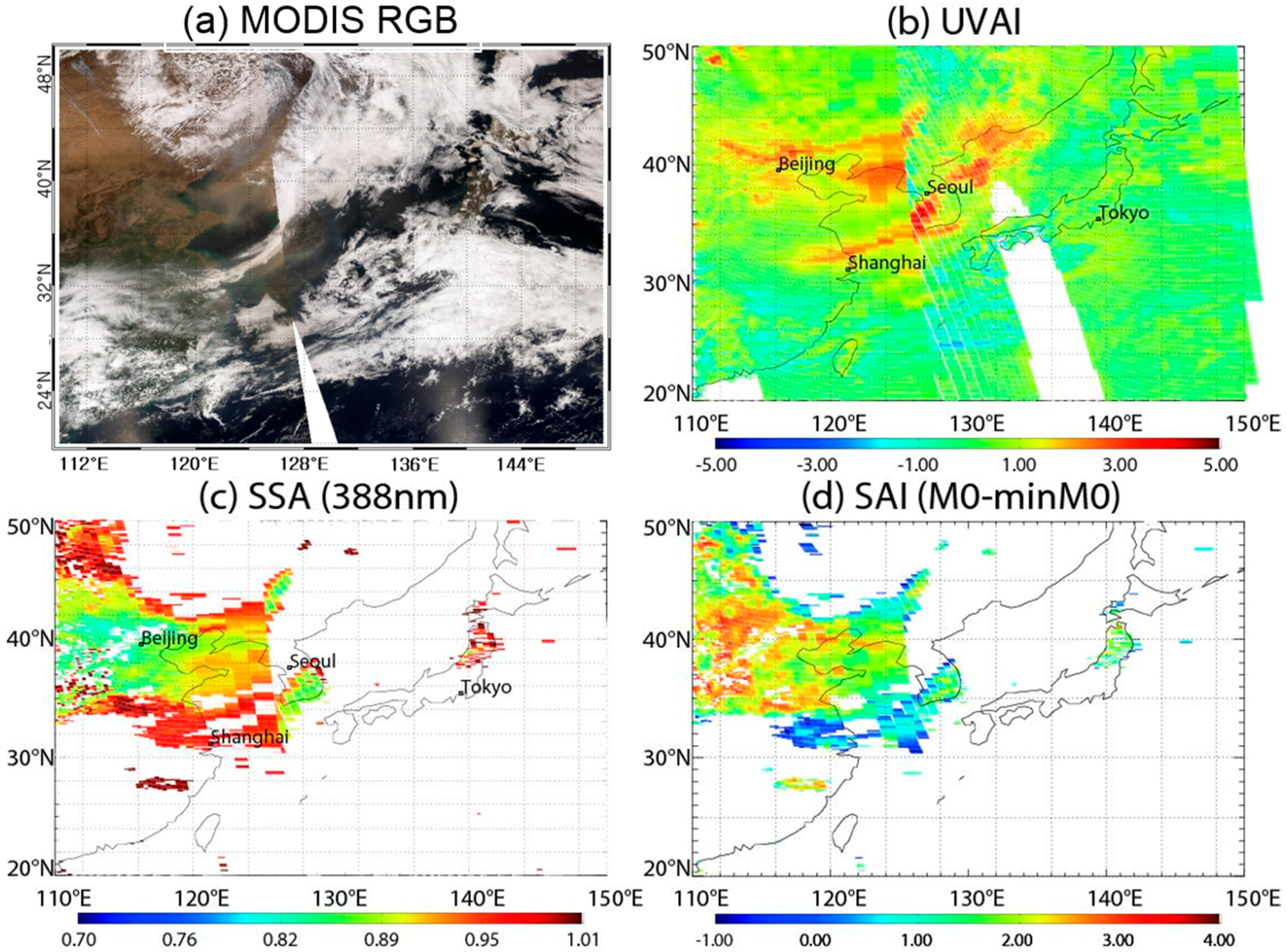
Figure 7.
(a–i) Results of an agreement and false detection test of OMI UVAI and OMI SAI for 8 April (Case 1) and 23 April (Case 2, Case 3) 2006, respectively. The x-axis indicates the SAI absorbing threshold ranging from −0.5 to 1.5. The different line styles indicate different UVAI threshold values. The SAI value of 0.5 corresponds to a UVAI value of 0.7. The false detection rate is constant, indicating that the current SAI algorithm correctly defines the absorbing aerosol pixels.
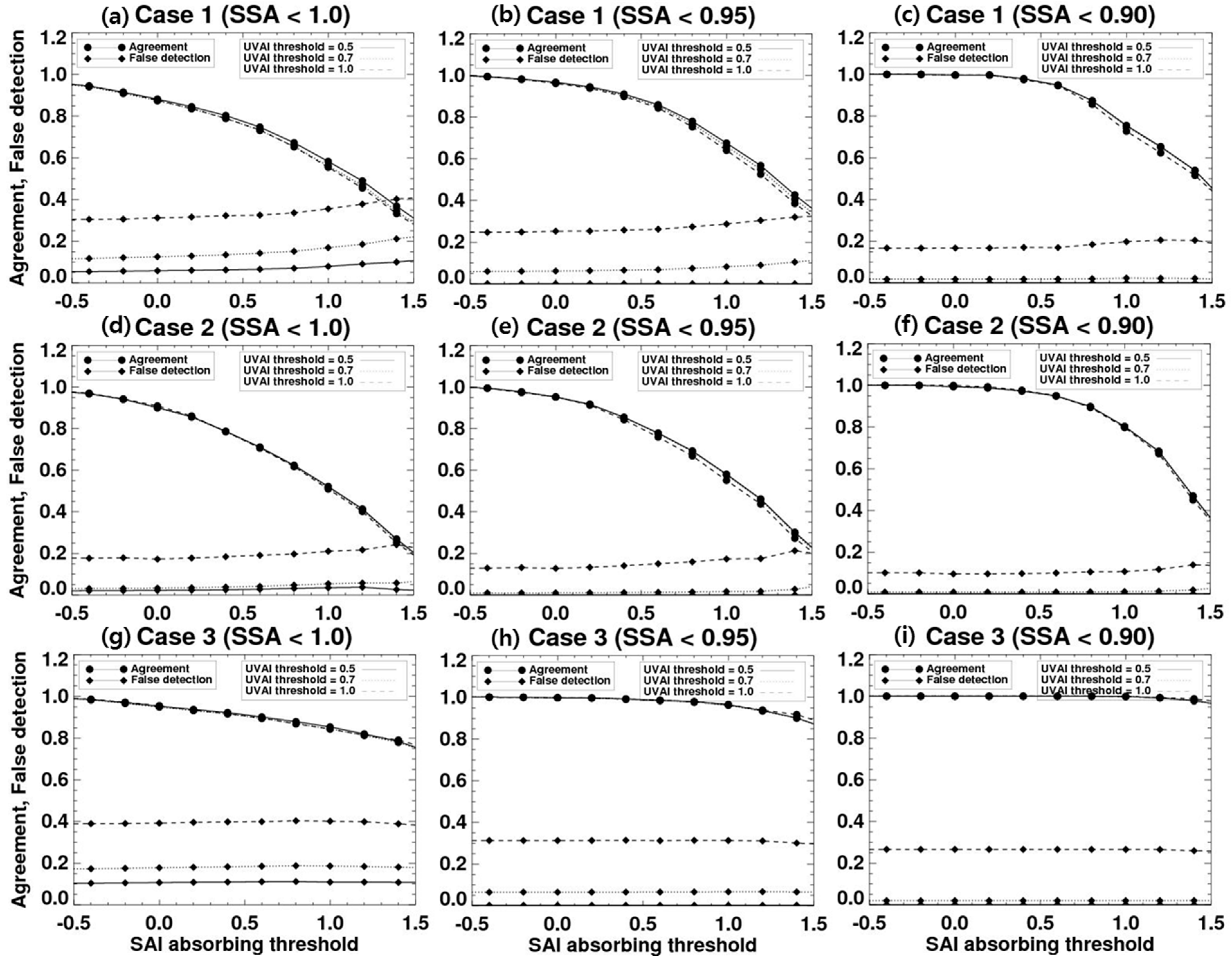
Figure 8.
OMI UVAI, SSA, and calculated TANSO-CAI SAI for UTC 04:29 on March 17 2012 over the Korean Peninsula. (a) MODIS RGB has an 8-min time difference compared with OMI; (b) A single path of OMI lv.2 UVAI (354 and 388 nm) data is projected; (c) OMI lv.2 SSA 388 nm (d) SAI calculated from TANSO-CAI has a 30-min time difference compared with OMI.
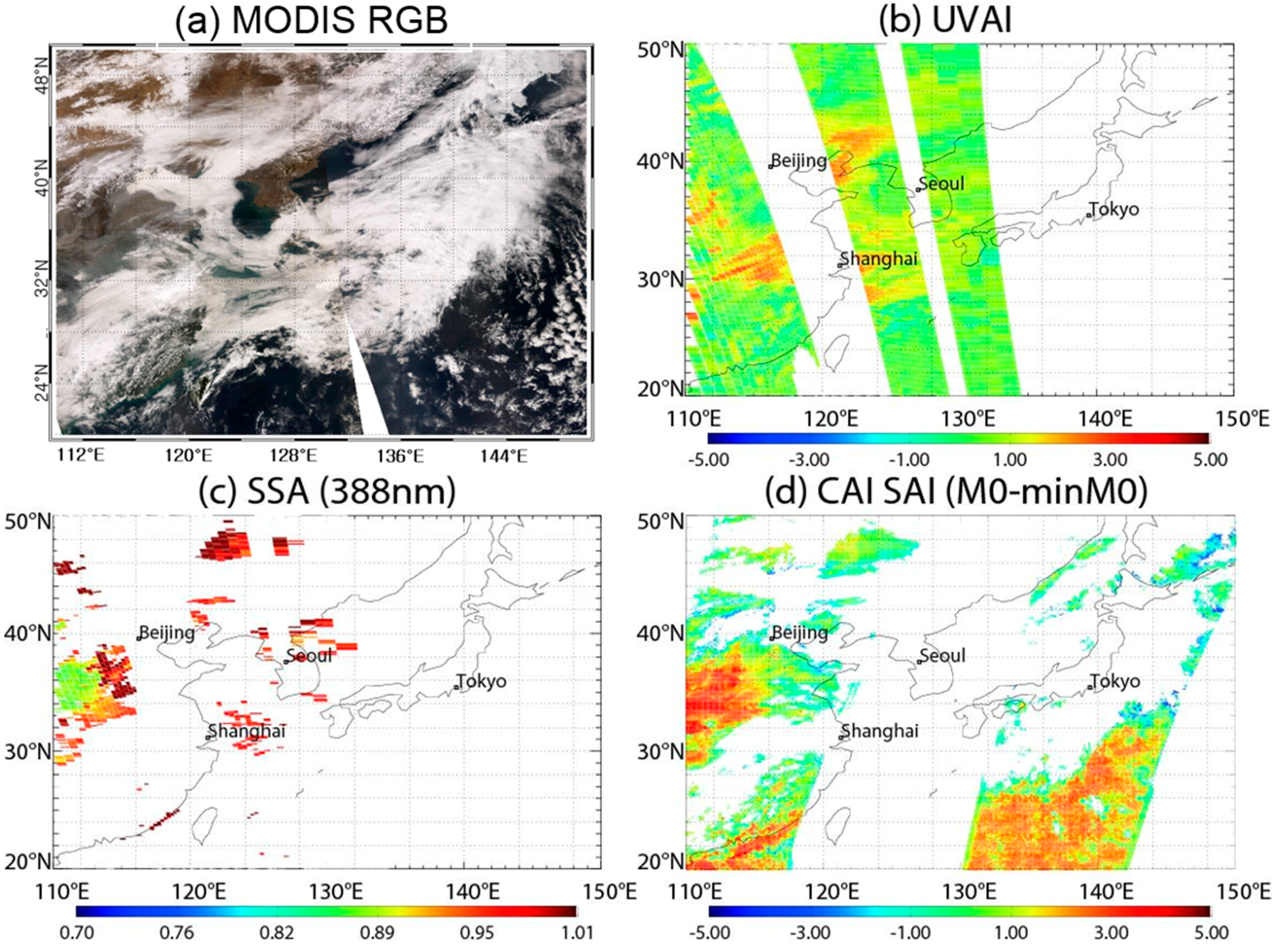
Figure 9.
OMI UVAI, SSA, and calculated CAI-SAI for UTC 04:40 on April 25 2012 over the Korean Peninsula. (a) MODIS RGB has an 8-min time difference compared with OMI; (b) A single path of OMI lv.2 UVAI (354 and 388 nm) data is projected. A sun-glint area near the south coast of China was removed because this area has a brighter surface than other ocean surface areas; (c) OMI lv.2 SSA 388 nm (d) SAI calculated from TANSO-CAI with a 30-min time difference compared with OMI.

Figure 10.
(a–d) Results of an agreement and false detection test of OMI UVAI and TANSO-CAI SAI for 17 March and 25 April 2012, respectively. The left column shows the results for OMI SSA values less than 1.0, while the right column shows the results for SSA values less than 0.95. The SAI value of 0.5 corresponds to a UVAI value of 0.7. The false detection rate is constant for moderate absorbing aerosol cases.


Table 1.
Number-Weighted Particle Size Distributions and Refractive Indices of Aerosol Models Employed to Retrieve the Theoretical Value of SAI and UVAI using VLIDORT.
Table 1.
Number-Weighted Particle Size Distributions and Refractive Indices of Aerosol Models Employed to Retrieve the Theoretical Value of SAI and UVAI using VLIDORT.
| TYPE | rm1 | rm2 | σm1 | σm2 | Fraction of m1 | Re(RI) (443 nm) |
|---|---|---|---|---|---|---|
| SMOKE | 0.080 | 1.005 | 1.644 | 1.849 | 0.9997 | 1.45 |
| DUST | 0.065 | 0.832 | 1.451 | 1.820 | 0.9978 | 1.52 |
| NA | 0.087 | 0.741 | 1.772 | 1.976 | 0.9997 | 1.42 |
Table 2.
Considered Parameters for LUT to Retrieve the Theoretical Value of SAI and UVAI using VLIDORT. SZA, RAA, and VZA are fixed to 36°, 150°, and 38°, respectively.
Table 2.
Considered Parameters for LUT to Retrieve the Theoretical Value of SAI and UVAI using VLIDORT. SZA, RAA, and VZA are fixed to 36°, 150°, and 38°, respectively.
| Variable | No. of Entries | Entries |
|---|---|---|
| Surface elevation | 3 | 0, 3, 6 km |
| Aerosol peak height | 5 | 0.5, 1.5, 3.0, 4.5, 6.0 km |
| AOD | 4 | 0, 1, 2, 3 |
| SSA (ref_wav = 443 nm) | 7 (SMOKE, DUST) 8 (NA) | 0.82, 0.85, 0.88, 0.91, 0.94, 0.96, 0.98 0.90, 0.92, 0.94, 0.96, 0.97, 0.98, 0.99, 1.0 |
| Wavelength | 2 | 354, 388 nm |
| Surface reflectance | 8 | 0.0, 0.01, 0.025, 0.05, 0.1, 0.3, 0.55, 0.8 |
Table 3.
Considered parameters for LUT to retrieve the SAI using OMI and CAI.
| Variable | No. of Entries | Entries |
|---|---|---|
| SZA | 8 | 0, 10, ..., 70 |
| RAA | 7 | 0, 30, ..., 180 |
| VZA | 8 | 0, 10, ..., 70 |
| Surface pressure | 6 | 600, 700, 800, 900, 1000, 1014 mb |
| AOD | 1 | 0 |
| Wavelength (OMI) Wavelength (CAI) | 2 41 | 354, 388 nm 360,361, ..., 400 nm |
| Surface reflectance | 8 | 0.0, 0.025, 0.05, 0.12, 0.25, 0.4, 0.55, 0.7 |
Table 4.
Six empirical SAI models (M0 to M5) are categorized with background AI marked in bold. Slopes and correlation coefficients of six empirical models with respect to SSA are presented. ‘20060408’ indicates the selected day and ‘t0400’ indicates the OMI passing time (in this case UTC 04:00). The empirical model (c) M0-minM0 showed the highest correlation coefficient and a linear relationship (see also Figure 4 and Figure 5).
| No. | Day | Before Cloud Screening | After Cloud Screening | ||||
|---|---|---|---|---|---|---|---|
| (a) M0 | (b) M1: M0-minM0 | (c) M2: M0-minM0 | (d) M3: M0-meanM0 | (e) M4: M0-medianM0 | (f) M5: M0-min(absM0) | ||
| 1 | 20060408 t0400 | y = −0.026x + 0.894 | y = −0.015x + 0.997 | y = −0.019x + 0.938 | y = −0.023x + 0.913 | y = −0.022x + 0.910 | y = −0.026x + 0.891 |
| R2 = 0.525 | R2= 0.427 | R2 = 0.399 | R2= 0.544 | R2 = 0.538 | R2 = 0.514 | ||
| 2 | 20060423 t0319 | y = −0.031x + 0.869 | y = −0.025x + 1.039 | y = −0.038x + 0.939 | y = −0.03x + 0.892 | y = −0.027x + 0.890 | y = −0.033x + 0.861 |
| R2 = 0.357 | R2 = 0.340 | R2 = 0.540 | R2 = 0.372 | R2 = 0.341 | R2 = 0.429 | ||
| 3 | 20060408 t0458 | y = −0.056x + 0.872 | y = −0.033x + 1.096 | y = −0.038x + 0.967 | y = −0.050x + 0.909 | y = −0.048x + 0.901 | y = −0.056x + 0.868 |
| R2 = 0.603 | R2 = 0.348 | R2 = 0.626 | R2 = 0.597 | R2 = 0.571 | R2 = 0.643 | ||
© 2017 by the authors. Licensee MDPI, Basel, Switzerland. This article is an open access article distributed under the terms and conditions of the Creative Commons Attribution (CC BY) license (http://creativecommons.org/licenses/by/4.0/).
Share and Cite
MDPI and ACS Style
Go, S.; Kim, M.; Kim, J.; Park, S.S.; Jeong, U.; Choi, M. Detection of Absorbing Aerosol Using Single Near-UV Radiance Measurements from a Cloud and Aerosol Imager. Remote Sens. 2017, 9, 378. https://doi.org/10.3390/rs9040378
AMA Style
Go S, Kim M, Kim J, Park SS, Jeong U, Choi M. Detection of Absorbing Aerosol Using Single Near-UV Radiance Measurements from a Cloud and Aerosol Imager. Remote Sensing. 2017; 9(4):378. https://doi.org/10.3390/rs9040378
Chicago/Turabian StyleGo, Sujung, Mijin Kim, Jhoon Kim, Sang Seo Park, Ukkyo Jeong, and Myungje Choi. 2017. "Detection of Absorbing Aerosol Using Single Near-UV Radiance Measurements from a Cloud and Aerosol Imager" Remote Sensing 9, no. 4: 378. https://doi.org/10.3390/rs9040378
Note that from the first issue of 2016, this journal uses article numbers instead of page numbers. See further details here.