Automatic Object-Oriented, Spectral-Spatial Feature Extraction Driven by Tobler’s First Law of Geography for Very High Resolution Aerial Imagery Classification

Abstract

Aerial image classification has become popular and has attracted extensive research efforts in recent decades. The main challenge lies in its very high spatial resolution but relatively insufficient spectral information. To this end, spatial-spectral feature extraction is a popular strategy for classification. However, parameter determination for that feature extraction is usually time-consuming and depends excessively on experience. In this paper, an automatic spatial feature extraction approach based on image raster and segmental vector data cross-analysis is proposed for the classification of very high spatial resolution (VHSR) aerial imagery. First, multi-resolution segmentation is used to generate strongly homogeneous image objects and extract corresponding vectors. Then, to automatically explore the region of a ground target, two rules, which are derived from Tobler’s First Law of Geography (TFL) and a topological relationship of vector data, are integrated to constrain the extension of a region around a central object. Third, the shape and size of the extended region are described. A final classification map is achieved through a supervised classifier using shape, size, and spectral features. Experiments on three real aerial images of VHSR (0.1 to 0.32 m) are done to evaluate effectiveness and robustness of the proposed approach. Comparisons to state-of-the-art methods demonstrate the superiority of the proposed method in VHSR image classification.

1. Introduction

Aerial imagery, including that from unmanned aerial vehicles (UAVs), has become increasingly popular. Its advantages, such as high spatial resolution, low cost, and ready availability, provide numerous potential applications [1,2,3]. Compared with low or median spatial resolution images, aerial images often have very high spatial resolution (VHSR). This provides more details of the earth surface, including the shape, structure, size, and texture of ground targets, and even topology and thematic information among targets. Therefore, a VHSR image is useful for investigating urban environments, target extraction, and urban land-cover mapping [4,5,6,7]. However, the higher resolution does not necessarily produce greater classification accuracies; VHSR image classification poses a challenge in practical application [8]. This is because if the spatial resolution is very fine, then the classification could not be improved anymore because of the within-class variability in spectral values. To conquer this problem, spatial feature extraction and complementing with spectral features are known to be important technique in VHSR image classification [9].

Spatial feature extraction is aimed at describing the shape, structure, and size of a target on the earth surface. However, the spatial arrangement of the ground targets is complex and uncertain. Many researchers have proposed threshold-based approaches to extract spatial features and improve the performance of VHSR image classification. For example, Han et al. considered the shape and size of a homogeneous area, selecting suitable spatial features using parameters [10]. Zhang et al. discussed a multiple shape feature set that can characterize the target using different points to enhance classification accuracy [11]. However, an “optimal” threshold for a given image cannot be determined until a series of experiments has been carried out, which is very time-consuming. Although such a threshold can be selected by experiment, one cannot know whether it is indeed the best for all images. Furthermore, such a single optimal threshold may not handle the various shapes in all image cases.

Besides threshold-based extension methods, a mathematical model is an effective means to treat contextual information for extracting spatial features. For example, Moser et al. extracted spatial-contextual information using the Markov random field (MRF) [12]. There is extensive literature on the use of MRF in VHSR image classification, such as [13,14,15]. Morphological profiles (MPs) represent another powerful tool for spatial feature extraction [16]. The structural element (SE) is crucial to morphological operations, so MPs have been extended in size and shape by many researchers [9,17]. Furthermore, MP attributes have been exploited for describing spatial features of VHSR images [18,19,20]. Among these methods, contextual information within a “window” around a central pixel is simulated and a mathematical model extracted, such as the MRF or MPs. However, the main limitations of considering a set of neighbors using a regular window are the following: (i) The regular neighborhood may not cover the various shapes of different targets in the varying classes, or even different targets within a single class; (ii) although extension of the MP in size or shape can improve the classification performance, it is still inadequate to fit the various shapes and sizes of ground targets in an image scene. Therefore, the adaptive ability of a spatial feature extraction approach should be studied extensively. Ideally, spatial feature extraction should be driven by the image data itself.

In recent decades, many literature works have revealed that image object-based image analysis was effective for that classification [21,22]. An image object is a group pixel set with similar spectral values, such that the object has homogeneous spectra. Compared with pixel-based methods, the object-based approach has two advantages: (i) Image objects have more usable features (e.g., shape, size and texture) than a single pixel; (ii) because the processing unit is improved from pixel to object, much “salt and pepper” noise can be smoothed in the classification results. For example, Zhao et al. proposed an algorithm integrating spectral, spatial contextual, and spatial location cues within a condition random field framework to improve the performance of VHSR image classification [23]. Zhang et al. proposed an object-based spatial feature called object correlative index (OCI) to improve land-cover classification [24]. Most of image object-based classification methods rely on the performance of segmentation [25]. However, the scale parameter of multi-resolution segmentation is difficult to determine [26]. In the present work, we integrated an image raster and its corresponding segment vector to use topological relationships and geographic characteristics, with the aim of extracting VHSR image spatial features automatically.

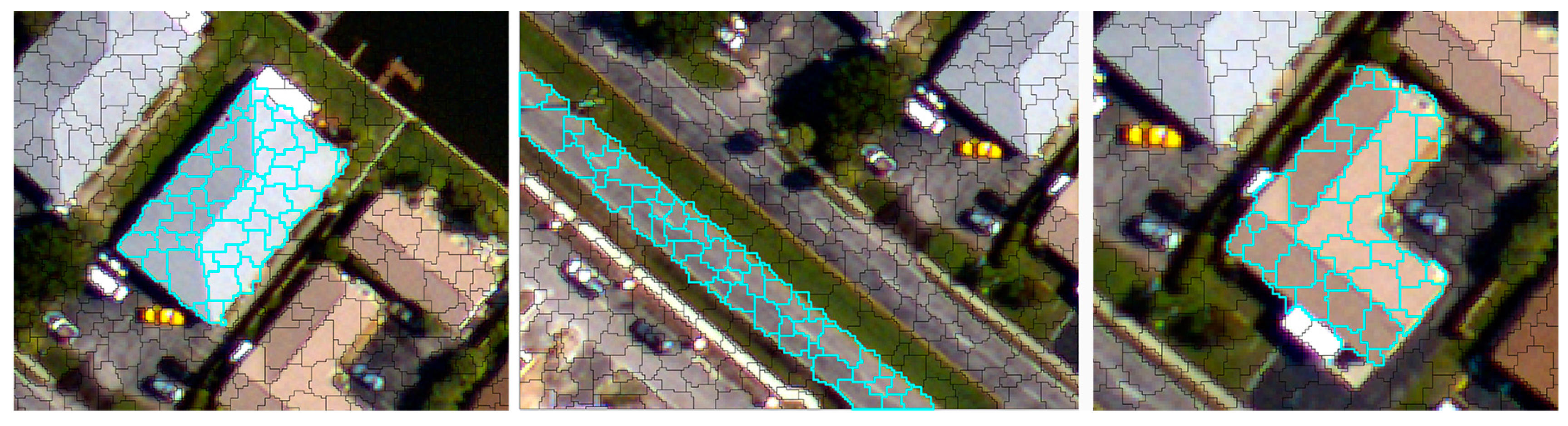
The proposed approach is based on two simple assumptions: (i) Objects making up a target are not only spatially continuous but are also more homogeneous in spectra than objects not belonging to the same target; (ii) objects from one target usually have very similar auto-correlation. As shown in Figure 1, objects comprising a ground target appear spectrally very similar, and are continuous in the spatial domain. Based on this observation, Tobler’s First Law of Geography (TFL) of geographic and topologic relationships of an object is used to constrain the extension for exploring the target region. One advantage of this combination is that it can better model the spatial arrangement of a target and effectively detect the target regardless of its shape or size (e.g., the rectangular or “L” shaped building or linear road in Figure 1). For the second assumption above (ii), Moran’s Index (MI) is typically used to quantitatively measure auto-correlation of the pixels for an object. Then, objects making up a target with similar (homonymous) MI are used to constrain the extension. In other words, the extension of a region for an uncertain target should be driven by the TFL of geography and the target itself, rather than parameter constraints. Experimental results demonstrate outstanding classification accuracy performance of the proposed feature extraction method. This means that the two basic assumptions based on observation of the ground target’s geography are very useful in feature extraction of VHSR aerial imagery.

The main goal of this paper was to propose an automatic object-based, spatial-spectral feature extraction method for VHSR image classification. With the aid of TFL of geography, that method extracts spatial features based on topology and spectral feature constraints, which are important to VHSR image classification. In more detail, the contributions of the method are as follows:

(i)

Contextual information of remote sensing imagery has been studied extensively and TFL has been widely applied in the field of geographic information systems (GIS). However, to the best of our knowledge, few approaches have been developed based on the TFL of geography for VHSR image classification in an object-manner. The present study proves that GIS spatial analysis can be used effectively for spatial feature extraction of VHSR images.

(ii)

When an image is processed by multi-scale segmentation, the topological relationship between a central object and surrounding objects becomes more complex, unlike a central pixel and its neighboring pixels (e.g., 4-connectivity or 8-connectivity). Another contribution of this study is its extension strategy based on topology and spectral feature constraints, which is adaptive and improves modeling of the shape and size of an uncertain target.

(iii)

Besides the segmentation, the progress of feature extraction is automatic, and no parameter adjustment is necessary during its application to classification. This opens up the possibility of widespread practical application to remote sensing imagery.

The remainder of this paper is organized as follows. In Section 2, TFL of geography is reviewed. In Section 3, the proposed feature extraction method is described. An experimental description is given in Section 4 and conclusions are given in Section 5.

2. Review of Tobler’s First Law of Geography

Here, we briefly review TFL. According to Waldo Tobler, the first law of geography is that “everything is related to everything else, but near things are more related than distant things” [27]. It is evident from this law that it was largely ignored and the quantitative revolution declined, but it gained prominence with the growth of GIS. Despite notable exceptions, it is hard to imagine a world in which the law is not true, and it provides a very useful principle for analyzing earth surface information [28]. The widespread application of geography today accommodates a variety of perspectives on the significance of this law [29,30]. Remote sensing imagery is obtained based on the radiance of specific source targets on the ground surface. Therefore, when an image is segmented into objects, those objects are related in the spatial and spectral domains. Thus, TFL of geography is applicable to image analysis.

To extract spatial features of images based on TFL of geography, it is necessary to quantitatively measure correlation among objects and pixels within an object. The MI, an index of spatial dependence, is common for specifically describing metrics of spatial autocorrelation. MI has positive values when TFL applies, is zero when neighboring values are as different as distant ones, and is negative when neighboring values are more different than distant ones [31]. MI of object o is defined in Equation (1), where $I_o^b$ is given in Equation (2).

$$I_O=\frac{1}{n}{\displaystyle \sum _{b=1}^{b=n}{I}_o^b}$$

(1)

$$I_o^b=\frac{N}{{\displaystyle \sum _{i,j}^{i=N,j=N}{w}_{ij}}}•\frac{{\displaystyle \sum _{i,j}^{i=N,j=N}{w}_{ij}(x_i^b-\overline{x^b})(x_j^b-\overline{x^b})}}{{\displaystyle \sum _i^{i=N}{(x_i^b-\overline{x^b})}^2}}$$

(2)

Here, b is the band index of the image and n is the total number of bands. N is the total number of pixels within the object. $x_i^b$ is a pixel value of band b within o. $w_{ij}$ is an element of a matrix of spatial weights; if x_i and x_j are neighbors, $w_{ij}=1$, otherwise $w_{ij}=0$. $\overline{x^b}$ is the mean of pixels within o.

The constraint-rule on the extension around a central object is analyzed further in Section 3. In particular, we had two objectives: (i) TFL of geography is introduced for spatial feature extraction of a VHSR image, and its feasibility investigated; (ii) to reduce the classification algorithm’s data dependence and expand application of the VHSR image, we advance a “rule-constraint” automatic feature extraction method based on TFL of geography, instead of the traditional parameter-based feature extraction approach. One important difference between TFL in our study and spatial contextual information related in existing approaches is that TFL is adopted as a “relaxing rule” in the description of neighboring information, while many existing approaches describe the spatial contextual information in a rigorous manner. In addition, the relaxing rule in our study is driven adaptively by the contextual information rather than by a preset parameter. Details of our proposed methods are presented in Section 3.

3. Proposed Approach

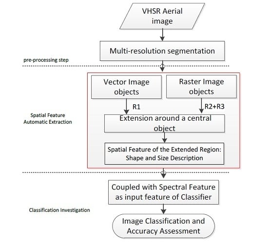
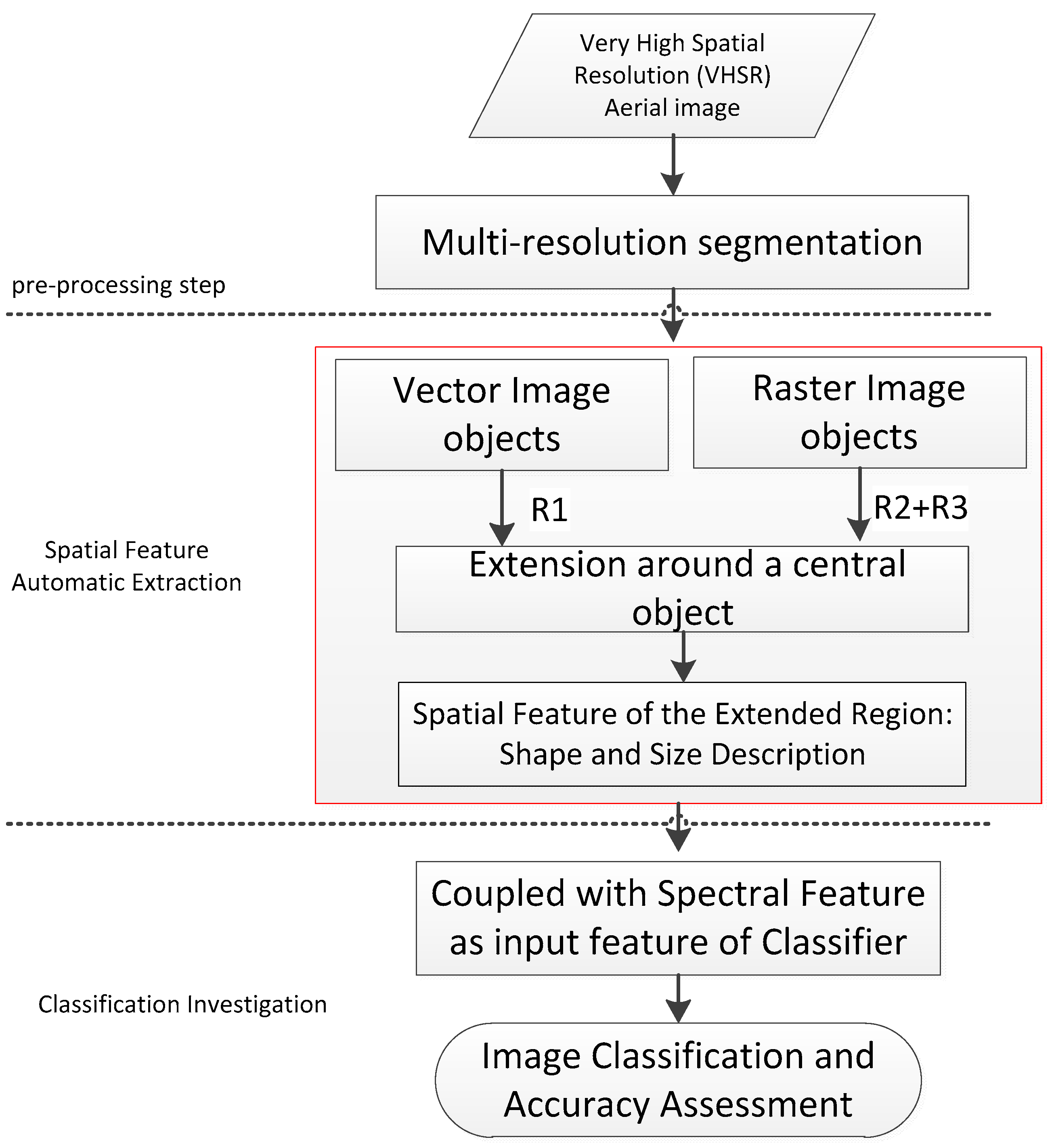
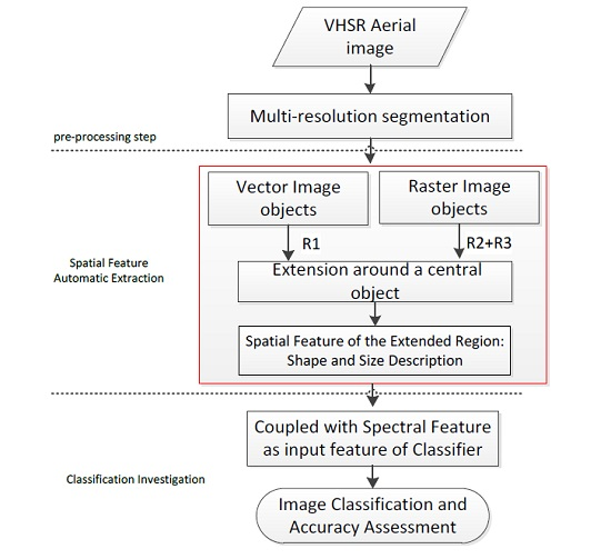
The proposed approach contains three main-blocks, as shown in Figure 2, they are: (1) Pre-processing step: In this paper, spatial features of a VHSR image are extracted in an object-by-object manner. Thus, image objects are first extracted using multi-resolution segmentation approach, which is embedded in the well-known eCogintion software [32]. The multi-resolution segmentation is an iterative region and bottom-up merging segmentation approach, and the merging process relies on local homogeneity by comparing adjacent objects within a certain radius [33]; (2) Spatial Feature Automatic Extraction: After segmentation, each image object is scanned and processed by an iterative procedure, as labeled by the red rectangle in Figure 2. The algorithm for the extension and spatial features for an extended region are described in the following sub-sections; (3) Classification Investigation: To test the accuracy and feasibility of the proposed automatic feature extraction approach, the proposed approach is compared with different spatial feature extraction approaches through land cover classification. Due to this, the concentration of this paper is to propose an automatic spatial feature extraction approach, the second block (spatial feature automatic extraction) will be detailed in the following sub-sections.

3.1. Extension Based on Constraint of TFL of Geography

Based on the segmentation results, a target may be composed of a group of correlative objects. Extension from one object of the group is used to extract the target region. However, target shape and size is uncertain in the spatial domain, and the objects in a group may vary spectrally and in homogeneity. Thus, it is difficult to constrain this extension by a determined parameter for a variety of target classes within an image scene. Here, three rules derived from TFL of geography are used to constrain the extension. To clarify this, symbols are explained in

Table 1. Explanation of symbols in the rule and its related algorithm.

Symbol	Explanation
$O_c$, $O_s$	These represent a central object ($O_c$) and surrounding object ($O_s$), respectively.
$\overline{m}\left(O_c\right)$, $\overline{m}\left(O_s\right)$	Mean of pixels within $O_c$ and $O_s$, respectively.
$\mathsf{\delta }\left(O_c\right)$	Standard deviation of pixels within an object, such as $O_c$.
$O_c^{+}$, $O_s^{+},O_R^{+}$	“+” means that the value of Moran’s index (MI) is positive for an object. e.g., $O_R^{+}$ means that the value of MI is positive for an explored region (a region is generated by explored objects in an extension)

.

Extension for a specific central object $O_c$ is done in an object manner, given that the following rules are satisfied. Each extension around $O_c$ is an iteration that is terminated depending on whether the relationship between $O_c$ and $O_s$ meets the following rules of constraint.

R1: $O_c$ and $O_s$ touch each other directly or indirectly in topology. “Indirectly” means that a connection has been built by previous extension between $O_s$ and $O_c$, but without direct touching.

R2: $\overline{m}\left(O_s\right)$ is in the range $\left[\overline{m}\left(O_c\right)-\mathsf{\delta }\left(O_c\right),\overline{m}\left(O_c\right)+\mathsf{\delta }\left(O_c\right)\right].$

R3: $O_s$ should meet the constraint $O_c^{+}\cup O_s^{+}=O_R^{+}$ or $O_c^{-}\cup O_s^{-}=O_R^{-}$. In other words, not only should $O_s$ and $O_c$ both have positive or negative MIs, but the explored region constructed by the extended objects should realize positive or negative MIs with its candidate component object $O_s$.

The details of these constraints used to explore the target region are shown in Algorithm 1 and Figure 3.

Algorithm 1. Extension of an object

Input: One of the segmented image object, ${\mathit{O}}_{\mathit{c}}$.

Output: A group of object sets that are surrounded ${\mathit{O}}_{\mathit{c}}$:${\mathit{O}}_{\mathit{R}}$.

1.  In the initialization step, ${\mathit{O}}_{\mathit{c}}$ is added to ${\mathit{O}}_{\mathit{R}}$. 2.  An object that touches ${\mathit{O}}_{\mathit{c}}$ in topology is collected in a container, which is designated by ${\mathit{O}}_{\mathit{c}\mathit{o}\mathit{n}}=\left\{{\mathit{O}}_1,{\mathit{O}}_2,{\mathit{O}}_3,\dots \dots {\mathit{O}}_{\mathit{T}}\right\}$;. 3.  A feature vector (${\mathit{V}}_{\mathit{c}}$) is built, based on mean values of band-1, band-2, band-3 and brightness of ${\mathit{O}}_{\mathit{c}}$, and ${\mathit{V}}_{\mathit{k}}$ ($1\le \mathit{k}\le \mathbf{T}$) is prepared for each object of ${\mathit{O}}_{\mathit{c}\mathit{o}\mathit{n}}$. The distance between ${\mathit{V}}_{\mathit{c}}$ and ${\mathit{V}}_{\mathit{k}}$ is compared, and the nearest-neighbor object ${\mathit{O}}_{\mathit{s}}$ is selected from ${\mathit{O}}_{\mathit{c}\mathit{o}\mathit{n}}$. 4.  If ${\mathit{O}}_{\mathit{s}}$ and ${\mathit{O}}_{\mathit{c}}$ meet the constrained rule R1, R2, and R3, ${\mathit{O}}_{\mathit{s}}$ is accepted as the “same-target-source” object while compared with ${\mathit{O}}_{\mathit{c}}$; 4.1. ${\mathit{O}}_{\mathit{s}}$ is added to ${\mathit{O}}_{\mathit{R}}$. At the same time, ${\mathit{O}}_{\mathit{s}}$ is used to replace ${\mathit{O}}_{\mathit{c}}$ for extension. 4.2. From step-1 through to step-4.1 is an iterative procedure. The iterative extension terminates when any of the three constraint rules is not satisfied. 5.  Else, terminate the extension and return ${\mathit{O}}_{\mathit{R}}$.

6.  Extension end.

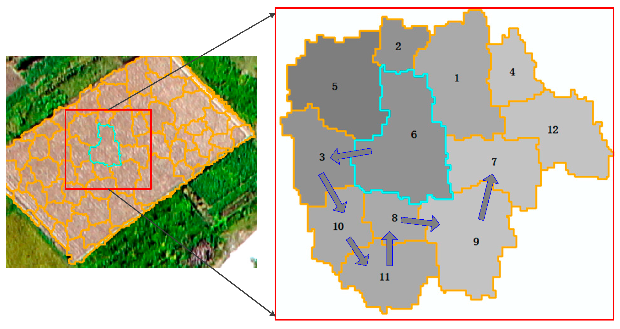
It should be noted that: (i) In each iteration, $O_c$ is replaced only for the extension in the spatial domain. The initial attribute of $O_c$, including its mean and standard deviation, are not varied in step-3 and the constraint rule (R2 and R3); (ii) according to TLF of geography, an object within the surrounding object set that achieves the nearest distance between itself and its central object is selected as the next central object for iteration, and distances are determined by (3). This is to ensure that the explored objects produce features similar to the central object $O_c$ in the attribute (feature) domain, but extend one by one in the spatial domain. As an example, in Figure 3, $O_6$ is highlighted as the central object, and it is readily seen that the region of a target soil can be extracted object-by-object using our proposed algorithm.

$$\Delta \mathrm{D}=\parallel v_o-v_s\parallel ,$$

(3)

where $\Delta D$ is the distance between the two vectors $v_o$ and $v_s$, $v_o$ is o’s feature vector, $v_o=\left\{{\overline{m}}_o^{b_1},{\overline{m}}_o^{b_2},{\overline{m}}_o^{b_3},{\overline{m}}_o^{bri}\right\}$, ${\overline{m}}_o^{b_1}$ is the mean value for band-1 pixels within o, and ${\overline{m}}_o^{bri}$ is the brightness of o. As with $v_o$, $v_s=\left\{{\overline{m}}_s^{b_1},{\overline{m}}_s^{b_2},{\overline{m}}_s^{b_3},{\overline{m}}_s^{bri}\right\}$.

The segmented vector is exported with the mean of the RGB band and brightnesses to a shape file. The vector layer is overlaid by the image raster for spatial analysis by our proposed algorithms. Application of the proposed algorithm was developed with the ESRI ArcGIS Engine 10.1 development kit and C# language.

3.2. Spatial Features: Shape and Size of Exploited Region

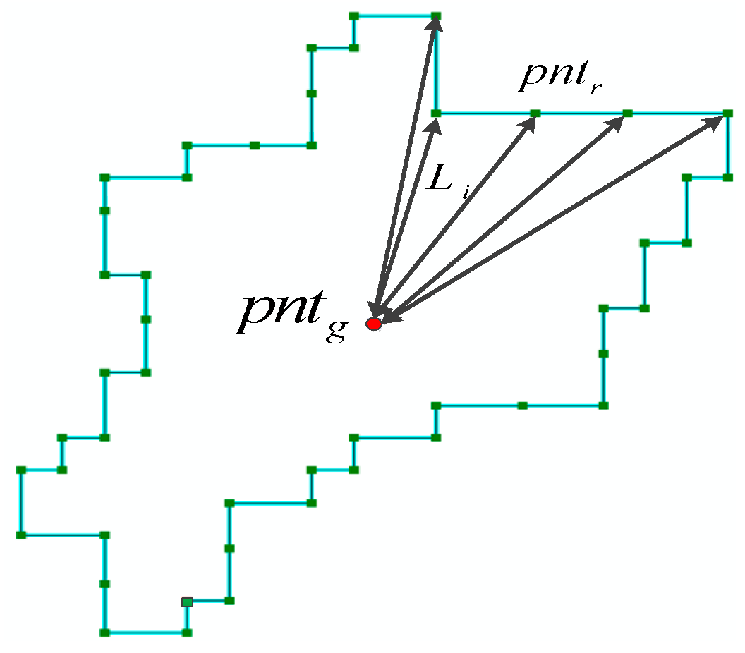
When iteration of an extension surrounding a central object is terminated, a homogenous and spatially continuous group of objects is output. To describe spatial features of the region composed by these grouped objects, a shape index (SI) and size-area (SA) are proposed, because shape and size are important for distinguishing various ground objects.

$$SI=\frac{1}{n}{\displaystyle \sum _{i=1}^{i=n}{L}_i},$$

(4)

where $L_i$ is distance between the gravity point ($pn{t}_g$) and region boundary point $pn{t}_r$, n is the total number of points on the region boundary, and n is determined by the interval distance and boundary length, as shown in Figure 4.

SA is given by

$$SA={\displaystyle \sum _{j=1}^{j=M}{a}_j^2},$$

(5)

where a is the image spatial resolution and $a^2$ is the area of a pixel. M is the total number of pixels within the extended region.

Each image object is scanned and processed by proposed Algorithm 1. Then, two spatial features, SI and SA, are extracted automatically to complement the spectral features for classification. The proposed method benefits from the following characteristics.

(i)

The segmented vector and image raster are integrated for spatial feature extraction, thereby demonstrating the novel concept that segmented vectors of topology and image features are both useful and feasible for VHSR image feature extraction.

(ii)

Three constraints and their related algorithms are driven based on the geographic theory of TFL. The proposed approach is automatic without any parameterization, thereby reducing data dependence and holding the promise of additional applications to VHSR image classification. It is worth noting that “automatic” means the progress of the feature extraction is automatic (excluding the segmentation and the supervised classification).

(iii)

The proposed approach based on TFL can adaptively extract the region of a target, because the extension around a central object is driven by the spatial contextual information itself.

4. Experiments

4.1. Experimental Datasets

To test the adaptive ability and effectiveness of our approach, we used three real aerial images with very high spatial resolution in experiments.

In the first experiment, to test the adaptive ability of our method for different classifiers, an aerial image was obtained from a UAV platform and Canon EOS 5D Mark II camera. Flight elevation was ~100 m and spatial resolution ~0.1 m. This image is 1400 × 1000 pixels. As shown in Figure 5a, seven classes were identified in the scene, i.e., roads, grass, buildings, shadow, trees, soil, and water.

The second aerial image was acquired by an ADS-80 sensor. The flight elevation is ~3 km and spatial resolution ~0.32 m, (Figure 5b). The image scene is 560 × 360 pixels and was classified into road, grass, buildings, shadow, trees, and water.

The third image (Figure 5c) was acquired in the same way as the first. The image is 1807 × 792 pixels and is of a typical urbanized area in China. It includes seven classes, i.e., roads, grass, buildings, shadow, trees, soil and water.

For the three datasets, classification was challenging because of lower spectral resolution and very high spatial resolution. The poorer spectral resolution limited the separation between classes. Furthermore, each dataset had very high spatial resolution, better than 0.3 m. Numerous studies have shown that higher spatial resolution does not mean greater interpretation accuracy, because salt-and-pepper noise is often more serious in the classification map of a VHSR image than that of a median-low resolution image.

4.2. Experimental Setup

Ground-truth datasets for the three images were interpreted manually, and are shown in Figure 6d, Figure 7h and Figure 8h. In addition, each training set for the images was randomly selected. They are shown in

Table 2. Number of training and test data for unmanned aerial vehicle (UAV) image-1.

Class		Training Object	Test Pixels
No.	Name
1	Roads	5	50,736
2	Grass	6	43,832
3	Building	16	211,085
4	Shadow	9	38,642
5	Tree	7	36,361
6	Soil	6	16,168
7	Water	4	51,133

,

Table 3. Number of training and test data for aerial imagery.

Class		Training Objects/Pixels	Test Pixels
No.	Name
1	Road	12/888	5791
2	Grass	15/1849	11,130
3	Building	10/819	32,831
4	Shadow	10/499	3374
5	Tree	4/577	4077
6	Water	15/1885	5447

and

Table 4. Number of training and test data for UAV image-2.

Class		Training Objects/Pixels	Test Pixels
No.	Name
1	Roads	6/2318	38,597
2	Grass	10/3973	95,333
3	Building	10/3581	246,448
4	Shadow	4/1829	26,640
5	Tree	8/3100	76,884
6	Soil	3/592	3300
7	Water	4/1573	68,431

. Training pixels are related to their corresponding objects. Taking Table 3 as an example, 12/888 indicates that 888 pixels correspond to 12 image objects.

In the first experiment, the adaptive ability of our approach was tested for different classifiers based on UAV image-1 (Figure 5a). Three classifiers were used in this experiment, a naive Bayes classifier (NBC), maximum likelihood classifier (MLC), and support vector machine (SVM). NBC is a popular probabilistic classifier based on Bayes’ theorem, with strong (naive) independence assumptions between features. MLC depends on maximum likelihood estimation for each class. The SVM classifier with radial basis function (RBF) kernel function and parameters is established by 5-fold cross-validation.

In the following two experiments, to investigate the effectiveness and advantages of our proposed method, several popular and relatively new spatial-feature extraction methods were compared with it. Similar to ours, these methods also use spatial neighboring information, including pixel- and object-based approaches. They are multi-shape structuring element morphological profiles (M-MPs) [9], attribute profiles (APs) [18], RFs [34], RGF [35], and OCI [24]. Each spatial feature was coupled with the original spectral feature and entered in the support vector machine (SVM) classifier. Parameters in these experiments are as follows, and each was determined by a trial-and-error approach.

In the second experiment, the aerial image (Figure 5b) with 0.32-m spatial resolution was used for comparison. Parameter setting for each approach was done as follows. Three SE shapes (“disk”, “square”, and “line”) of size 6 × 6 size were used for the M-MPs. Structuring features of each band were extracted by M-MPs. Area features were extracted by APs with parameter list [49.0, 169.0, 361.0, 625.0, 961.0, 1369.0, 1849.0, 2401.0]. Three parameters used here for RFs are ${\delta }_s=200, {\delta }_r=30$ and iteration = 3. ${\delta }_s=3, {\delta }_r=0.05$, and iterations = 3 were set for RGF. Parameter in the OCI-based approach were set to $\mathsf{\theta }=20,T_1=20, T_2=45$. For a fair comparison, each spatial feature was coupled with the original spectral bands in the classification. SVM with RBF was used as a classifier, and 5-fold cross-validation used for parameter optimization.

In the third experiment, to test the adaptability of our approach, UAV image-2 (Figure 5c) with 0.1-m spatial resolution was used. As in the first experiment, the M-MP parameters had the same three SE shapes, but of size 8 × 8. To extract area features for individual targets, AP parameters were [49.0, 169.0, 361.0, 625.0, 961.0, 1369.0, 1849.0, 2401.0]. Three parameters used here for RFs were ${\delta }_s=200, {\delta }_r=40$ and iteration = 3. ${\delta }_s=5, {\delta }_r=0.05$, and iteration = 3 were set for RGF. Parameters in the OCI-based approach were set to $\mathsf{\theta }=20,T_1=15, T_2=45$.

4.3. Accuracy Evaluation

To evaluate the results of the proposed approach, three accuracy measures were adopted in accord with previous works [34]. The first measure is overall accuracy (OA), which is the percentage of pixels that are classified correctly. The second is average accuracy (AA), which is the mean percentage of correctly classified pixels in each specific class. The third measure is the kappa coefficient (Ka). Ka is the percentage of agreement corrected by the number of agreements that would be expected by chance [36]. OA, AA, and Ka are widely used to measure classification accuracy, and more details regarding them are found in the literature [9].

4.4. Results

The adaptive ability of our approach was evaluated in the first experiment by a UAV image with spatial resolution ~0.1 m. It was tested for the three classical classifiers SVM, MLC, and NBC. Comparison results are shown in Figure 6, and specific class and overall accuracies in

Table 5. Class-specific accuracies (%) for various classifiers and UAV image-1.

Class	MLC	NBC	SVM
Road	100.0	99.8	99.2
Grass	87.5	88.9	93.6
Building	69.7	94.5	94.4
Shadow	99.5	99.2	92.9
Tree	80.8	42.3	70.1
Soil	100.0	84.0	98.7
Water	100.0	86.0	97.7
OA	76.4	85.3	92.7
AA	91.1	85.0	92.4
Ka	0.635	0.796	0.898

. It is evident that the approach performed better with respect to the MLC, NBC, and SVM classifiers, with their respective OAs at 76.4%, 85.3%, and 92.7%. This reveals that the proposed feature extraction is robust for the three supervised classifiers.

The second experiment was performed on the aerial image with 0.32-m spatial resolution (Figure 5b). Table 3 presents the number of training and ground truth datasets. The training dataset accounting for ~10% of ground truth was chosen randomly. Figure 7 shows classification results from different spatial-spectral features, using the same SVM classifier, training, and ground-truth datasets. Classification accuracies are shown in

Table 6. Class-specific accuracies (%) for features in SVM classification of aerial image data.

Class	Spectral Feature Only	M-MPs	APs	RFs	RGF	OCI	Proposed
Road	36.9	65.6	29.0	86.1	83.0	90.3	47.3
Grass	79.1	80.1	76.7	81.3	71.3	91.6	92.6
Building	99.5	99.9	98.6	99.9	100.0	77.5	94.3
Shadow	66.6	22.1	84.7	19.4	19.0	82.2	64.8
Tree	80.2	99.9	77.0	99.7	99.9	59.8	79.2
Water	74.2	90.3	97.9	91.4	86.1	96.1	89.3
OA	73.7	72.8	70.6	72.7	71.9	81.8	82.3
AA	72.7	76.3	77.3	79.6	76.5	77.2	77.9
Ka	0.654	0.652	0.617	0.652	0.639	0.745	0.751

. As shown in the figure and table, compared with the original spectral feature, M-MPs, APs, RFs, RGF, and OCI spatial-spectral feature extraction methods, our approach gave the maximum classification accuracy. This demonstrates that our object-spatial-spectral feature approach driven by TFL of geography is feasible and effective for classification of VHSR imagery.

The third experiment was conducted using UAV image-2 with 0.1-m spatial resolution (Figure 5c). Table 4 presents numbers of training and test data. Figure 8 shows classification results of the SVM classifier using different spatial-spectral feature extraction approaches and the original spectral feature-only method. From Figure 8, the original spectral feature method produced much noise in the classification map, and the AP technique could not effectively remove noise pixels. Although M-MPs removed many noise pixels, more targets were misclassified, e.g., one building was classified into two parts, shadow and building. Furthermore, numerous small targets, such as shadows surrounding trees and between two buildings, were both removed by the M-MPs approach. There were similar classification results from the RF- and RGF-based approaches. Our approach performed better than using only spectral features, and the spatial-spectral feature extraction methods M-MPs, APs, RFs, RGF, and OCI. Quantitative comparisons are listed in

Table 7. Class-specific accuracies (%) for features in SVM classification of UAV image-2.

Class	Spectral Feature Only	M-MPs	APs	RFs	RGF	OCI	Proposed
Road	97.3	99.6	99.6	98.8	96.7	99.6	98.1
Grass	68.0	96.6	67.2	87.6	59.9	78.6	80.2
Building	99.8	99.8	82.1	100.0	99.8	82.4	97.0
Shadow	22.7	24.5	38.5	31.0	28.8	87.0	56.1
Tree	58.2	67.2	29.8	39.4	67.9	84.2	75.2
Soil	77.9	62.7	14.2	18.3	90.6	83.5	91.8
Water	98.4	100.0	43.9	98.5	99.0	86.4	88.1
OA	77.8	83.8	53.5	68.7	75.8	83.9	86.9
AA	74.6	78.6	53.6	67.7	77.5	81.6	83.8
Ka	0.711	0.79	0.426	0.607	0.69	0.79	0.823

, further demonstrating the advantages of our approach in terms of OA, AA, and Ka classification accuracies.

4.5. Discussion

In the first experiment, sensitivity of the segmental scale and training sample size to the proposed approach was investigated extensively as follows.

(i)

To obtain more homogeneous image objects and address segmental scale sensitivity, the parameters compactness and shape were fixed at 0.8 and 0.9. A smaller scale means more and relatively more homogeneous segmental objects. In this context, the relationship between segmental sale and classification accuracy was investigated. As shown in Figure 9, the OA range was 88.4% to 93.3%, while that of segmental scale was 5 to 35. When the segmental scale was >35, the accuracy sharply decreased, which may be have been produced by under-segmentation. This indicates that the proposed approach is relatively robust to segmental scale. This is because the approach has an advantage in searching the adaptive spatial region for an uncertain target.

(ii)

Another factor that affects the classification is training sample size. To investigate the sensitivity to this size for accuracy, the segmental scale was fixed at 20. As shown in Figure 10, the OA ranged from 82.1% to 84.2% with training size varying between 30 and 80. While the size of training samples was >100, OA increased up to 93.3% and had a stable trend. AA and Ka exhibited a similar result. Overall, the approach could achieve satisfactory accuracy with a relatively small training sample size, e.g., when that size was 30 objects and candidate objects numbered 6026, OA = 84.2%, AA = 88.2, and Ka = 0.774.

Overall, by comparing classification performance of Experiment-2 and Experiment-3, it is clear that the spatial feature was beneficial for complementing spectral features to improve VHSR image land-cover classification. Furthermore, from these experimental results, the object-based spatial feature was competitive with the pixel-based spatial feature in land-cover classification. Upon comparing the proposed approach with the OCI-based spatial-spectral feature method, the proposed approach achieved higher classification accuracies. Moreover, there was no parameter which had to be adjusted for feature-extraction. An automatic object-based image feature-extraction approach is useful for promoting its widespread application in land-cover classification. The improvements and benefits of the proposed approach mainly come from the proposed search strategy and constraint rules, which are inspired by the intrinsic TFL law. However, it should be noted that parameters are necessary for the segmentation which is an initial but essential step for generating object. When trial-and-error method is adopted for parameters’ optimization of segmentation, it must be based on the using of available ground truth data or prior knowledge.

5. Conclusions

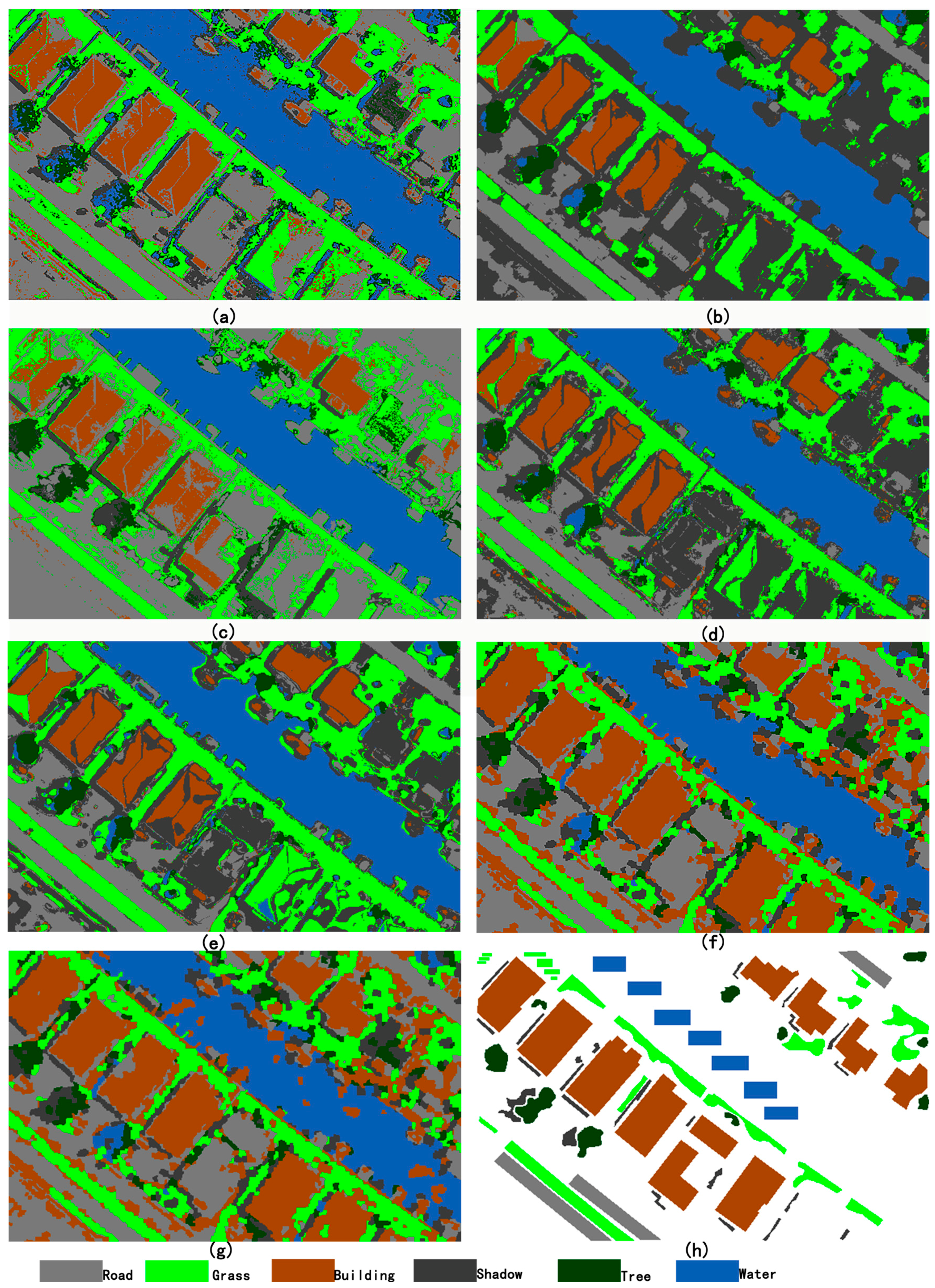
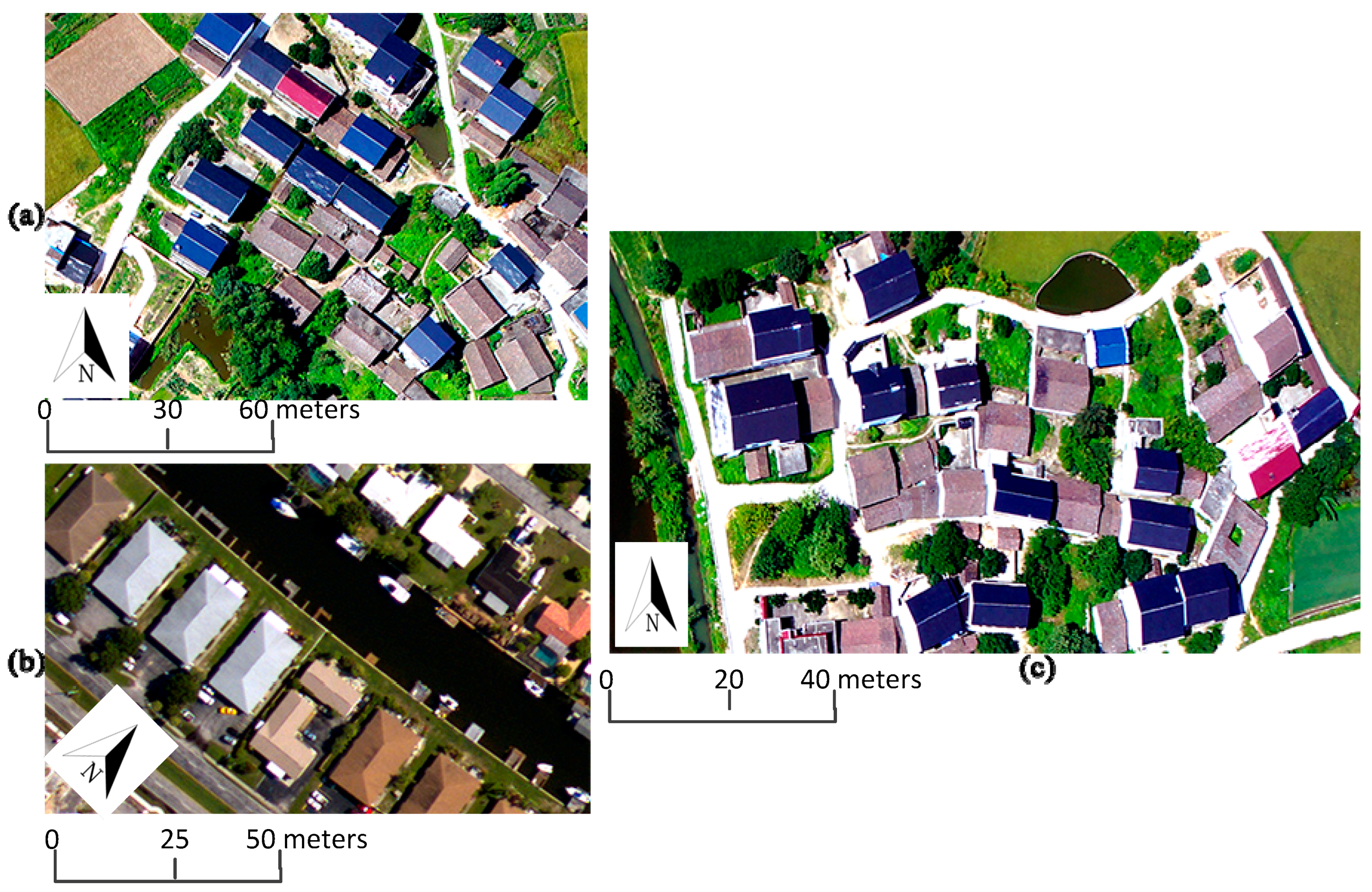
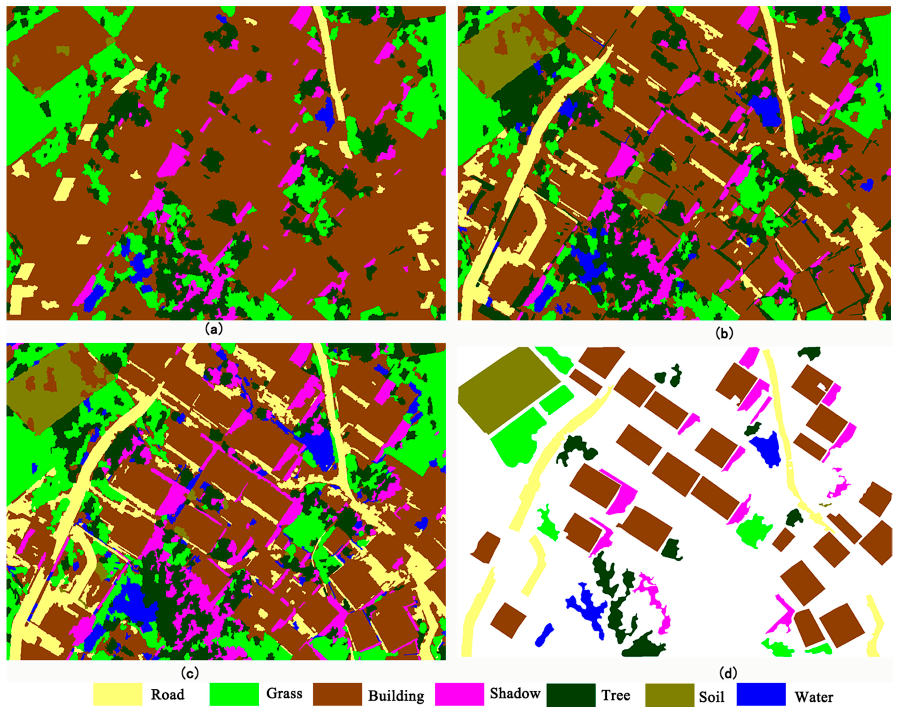
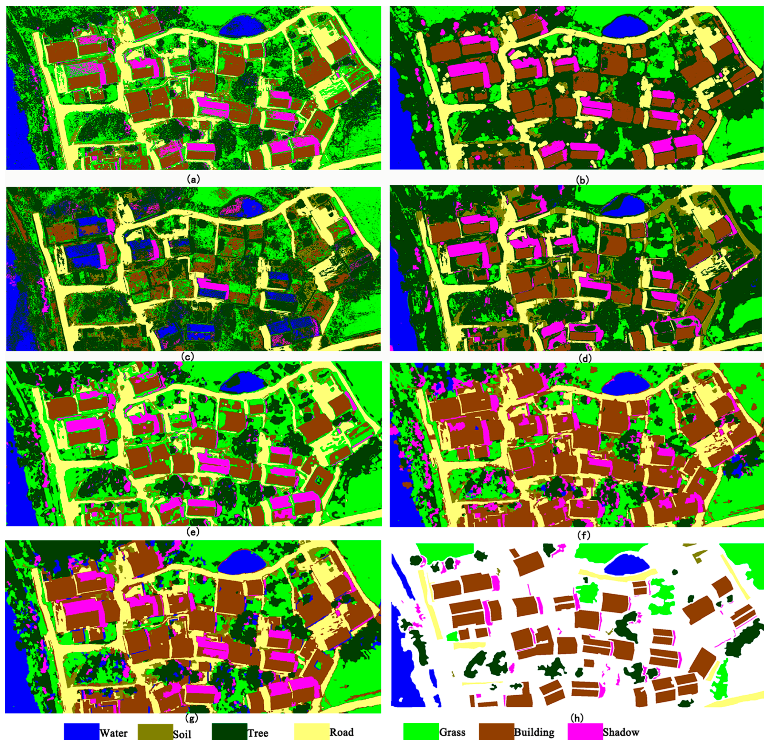
In this work, an automatic object-based, spatial-spectral feature extraction approach was proposed for the classification of VHSR aerial imagery. The proposed approach was inspired by TFL of geography to constrain the extent of region exploration. Two spatial features, SI and SA, are proposed for describing the region until the extension is terminated. Experiments were conducted on three actual VHSR aerial images. The experimental results demonstrate the effectiveness of our approach, which gave results superior to those from the use of only original spectral features, the widely used spatial-spectral method, M-MPs, APs, RFs, RGF, and OCI.

Based on the findings of this work from analysis and experiment, we conclude that, the TFL of geography can be used for quantitative image feature extraction from VHSR imagery, which contains spatial data describing the land cover on the earth surface. Moreover, although the two types of spatial data (raster and vector) are very different in their characteristics, they can be integrated with the aid of intrinsic geography. This is helpful for better modeling of the spatial features of VHSR images.

Furthermore, from the perspective of practical application, the proposed feature extraction approach without a parameter is simple and data-dependent, which will lead to more potential applications. With the development of UAV technology, large numbers of VHSR images can be acquired conveniently, and classification is important in practical application [37]. Further development of this work will include comprehensive research on the topological relationship between objects. In addition, because the smaller zone that is meaningless compared with the object of interest, and which can be seen as containing “noise objects,” has a negative effect on classification performance and accuracy, knowledge-based rules driven by expert experience will be considered for optimizing the post-classified map.

References

1. Zhang, L.; Han, Y.; Yang, Y.; Song, M.; Yan, S.; Tian, Q. Discovering discriminative graphlets for aerial image categories recognition. IEEE Trans. Image Process. 2013, 22, 5071–5084. [Google Scholar] [CrossRef] [PubMed]
2. Huang, W.; Wu, L.; Wei, Y.; Song, H. Order based feature description for high-resolution aerial image classification. Opt. Int. J. Light Electron Opt. 2014, 125, 7239–7243. [Google Scholar] [CrossRef]
3. Cheriyadat, A.M. Unsupervised feature learning for aerial scene classification. IEEE Trans. Geosci. Remote Sens. 2014, 52, 439–451. [Google Scholar] [CrossRef]
4. Ardila, J.P.; Bijker, W.; Tolpekin, V.A.; Stein, A. Context-sensitive extraction of tree crown objects in urban areas using vhr satellite images. Int. J. Appl. Earth Obs. Geoinf. 2012, 15, 57–69. [Google Scholar] [CrossRef]
5. Du, S.; Zhang, F.; Zhang, X. Semantic classification of urban buildings combining VHR image and GIS data: An improved random forest approach. ISPRS J. Photogramm. Remote Sens. 2015, 105, 107–119. [Google Scholar] [CrossRef]
6. Li, M.; Stein, A.; Bijker, W.; Zhan, Q. Region-based urban road extraction from VHR satellite images using binary partition tree. Int. J. Appl. Earth Obs. Geoinf. 2016, 44, 217–225. [Google Scholar] [CrossRef]
7. Tao, J.; Shu, N.; Wang, Y.; Hu, Q.; Zhang, Y. A study of a gaussian mixture model for urban land-cover mapping based on vhr remote sensing imagery. Int. J. Remote Sens. 2016, 37, 1–13. [Google Scholar] [CrossRef]
8. Huang, X.; Zhang, L. An svm ensemble approach combining spectral, structural, and semantic features for the classification of high-resolution remotely sensed imagery. IEEE Trans. Geosci. Remote Sens. 2013, 51, 257–272. [Google Scholar] [CrossRef]
9. Lv, Z.Y.; Zhang, P.; Benediktsson, J.A.; Shi, W.Z. Morphological profiles based on differently shaped structuring elements for classification of images with very high spatial resolution. IEEE J. Sel. Top. Appl. Earth Obs. Remote Sens. 2014, 7, 4644–4652. [Google Scholar] [CrossRef]
10. Han, Y.; Kim, H.; Choi, J.; Kim, Y. A shape–size index extraction for classification of high resolution multispectral satellite images. Int. J. Remote Sens. 2012, 33, 1682–1700. [Google Scholar] [CrossRef]
11. Zhang, H.; Shi, W.; Wang, Y.; Hao, M.; Miao, Z. Classification of very high spatial resolution imagery based on a new pixel shape feature set. IEEE Geosci. Remote Sens. Lett. 2014, 11, 940–944. [Google Scholar] [CrossRef]
12. Moser, G.; Serpico, S.B.; Benediktsson, J.A. Land-cover mapping by Markov modeling of spatial–contextual information in very-high-resolution remote sensing images. Proc. IEEE 2013, 101, 631–651. [Google Scholar] [CrossRef]
13. Moser, G.; Serpico, S.B. Combining support vector machines and Markov random fields in an integrated framework for contextual image classification. IEEE Trans. Geosci. Remote Sens. 2013, 51, 2734–2752. [Google Scholar] [CrossRef]
14. Ghamisi, P.; Benediktsson, J.A.; Cavallaro, G.; Plaza, A. Automatic framework for spectral–spatial classification based on supervised feature extraction and morphological attribute profiles. IEEE J. Sel. Top. Appl. Earth Obs. Remote Sens. 2014, 7, 2147–2160. [Google Scholar] [CrossRef]
15. Zhao, J.; Zhong, Y.; Zhang, L. Detail-preserving smoothing classifier based on conditional random fields for high spatial resolution remote sensing imagery. IEEE Trans. Geosci. Remote Sens. 2015, 53, 2440–2452. [Google Scholar] [CrossRef]
16. Benediktsson, J.A.; Pesaresi, M.; Amason, K. Classification and feature extraction for remote sensing images from urban areas based on morphological transformations. IEEE Trans. Geosci. Remote Sens. 2003, 41, 1940–1949. [Google Scholar] [CrossRef]
17. Benediktsson, J.A.; Palmason, J.A.; Sveinsson, J.R. Classification of hyperspectral data from urban areas based on extended morphological profiles. IEEE Trans. Geosci. Remote Sens. 2005, 43, 480–491. [Google Scholar] [CrossRef]
18. Dalla Mura, M.; Benediktsson, J.A.; Waske, B.; Bruzzone, L. Morphological attribute profiles for the analysis of very high resolution images. IEEE Trans. Geosci. Remote Sens. 2010, 48, 3747–3762. [Google Scholar] [CrossRef]
19. Falco, N.; Benediktsson, J.A.; Bruzzone, L. Spectral and spatial classification of hyperspectral images based on ica and reduced morphological attribute profiles. IEEE Trans. Geosci. Remote Sens. 2015, 53, 6223–6240. [Google Scholar] [CrossRef]
20. Ghamisi, P.; Dalla Mura, M.; Benediktsson, J.A. A survey on spectral–spatial classification techniques based on attribute profiles. IEEE Trans. Geosci. Remote Sens. 2015, 53, 2335–2353. [Google Scholar] [CrossRef]
21. Arvor, D.; Durieux, L.; Andrés, S.; Laporte, M.-A. Advances in geographic object-based image analysis with ontologies: A review of main contributions and limitations from a remote sensing perspective. ISPRS J. Photogramm. Remote Sens. 2013, 82, 125–137. [Google Scholar] [CrossRef]
22. Blaschke, T.; Hay, G.J.; Kelly, M.; Lang, S.; Hofmann, P.; Addink, E.; Feitosa, R.Q.; van der Meer, F.; van der Werff, H.; van Coillie, F. Geographic object-based image analysis—Towards a new paradigm. ISPRS J. Photogramm. Remote Sens. 2014, 87, 180–191. [Google Scholar] [CrossRef] [PubMed]
23. Zhao, J.; Zhong, Y.; Shu, H.; Zhang, L. High-resolution image classification integrating spectral-spatial-location cues by conditional random fields. IEEE Trans. Image Process. 2016, 25, 4033–4045. [Google Scholar] [CrossRef] [PubMed]
24. Zhang, P.; Lv, Z.; Shi, W. Object-based spatial feature for classification of very high resolution remote sensing images. IEEE Geosci. Remote Sens. Lett. 2013, 10, 1572–1576. [Google Scholar] [CrossRef]
25. Liu, D.; Xia, F. Assessing object-based classification: Advantages and limitations. Remote Sens. Lett. 2010, 1, 187–194. [Google Scholar] [CrossRef]
26. Johnson, B.A.; Bragais, M.; Endo, I.; Magcale-Macandog, D.B.; Macandog, P.B.M. Image segmentation parameter optimization considering within-and between-segment heterogeneity at multiple scale levels: Test case for mapping residential areas using landsat imagery. ISPRS Int. J. Geo Inf. 2015, 4, 2292–2305. [Google Scholar] [CrossRef]
27. Tobler, W.R. A computer movie simulating urban growth in the detroit region. Econ. Geogr. 1970, 46, 234–240. [Google Scholar] [CrossRef]
28. Miller, H.J. Tobler’s first law and spatial analysis. Ann. Assoc. Am. Geogr. 2004, 94, 284–289. [Google Scholar] [CrossRef]
29. Griffith, D.A. Spatial Autocorrelation and Spatial Filtering: Gaining Understanding through Theory and Scientific Visualization; Springer Science & Business Media: Berlin, Germany, 2013. [Google Scholar]
30. Rousset, F.; Ferdy, J.B. Testing environmental and genetic effects in the presence of spatial autocorrelation. Ecography 2014, 37, 781–790. [Google Scholar] [CrossRef]
31. Li, H.; Calder, C.A.; Cressie, N. Beyond moran’s I: Testing for spatial dependence based on the spatial autoregressive model. Geogr. Anal. 2007, 39, 357–375. [Google Scholar] [CrossRef]
32. Baatz, M.; Schäpe, A. Multiresolution segmentation: An optimization approach for high quality multi-scale image segmentation. Angew. Geogr. Inf. XII 2000, 58, 12–23. [Google Scholar]
33. Benz, U.C.; Hofmann, P.; Willhauck, G.; Lingenfelder, I.; Heynen, M. Multi-resolution, object-oriented fuzzy analysis of remote sensing data for gis-ready information. ISPRS J. Photogramm. Remote Sens. 2004, 58, 239–258. [Google Scholar] [CrossRef]
34. Kang, X.; Li, S.; Benediktsson, J.A. Feature extraction of hyperspectral images with image fusion and recursive filtering. IEEE Trans. Geosci. Remote Sens. 2014, 52, 3742–3752. [Google Scholar] [CrossRef]
35. Xia, J.; Bombrun, L.; Adali, T.; Berthoumieu, Y.; Germain, C. Classification of hyperspectral data with ensemble of subspace ica and edge-preserving filtering. In Proceedings of the 2016 IEEE International Conference on Acoustics, Speech and Signal Processing (ICASSP), Shanghai, China, 20–25 March 2016; pp. 1422–1426.
36. Congalton, R.G. A review of assessing the accuracy of classifications of remotely sensed data. Remote Sens. Environ. 1991, 37, 35–46. [Google Scholar] [CrossRef]
37. Bhardwaj, A.; Sam, L.; Martín-Torres, F.J.; Kumar, R. UAVs as remote sensing platform in glaciology: Present applications and future prospects. Remote Sens. Environ. 2016, 175, 196–204. [Google Scholar] [CrossRef]
Figure 1. Examples taken from aerial images with three false-color bands and 0.32-m spatial resolution. From left to right, objects of three targets with different shapes are respectively highlighted.
Remotesensing 09 00285 g001
Figure 2. Schematic of proposed Tobler’s First Law of Geography (TFL)-based classification method.
Remotesensing 09 00285 g002
Figure 3. An extension example based on rule constraint. Highlighted object-6 is the central object; 6 3 10 11 8 9 7 is the order of extension, shown by blue-dotted arrow.
Remotesensing 09 00285 g003
Figure 4. Shape described by length between gravity point and boundary points.
Remotesensing 09 00285 g004
Figure 5. Experiment very high spatial resolution (VHSR) images: (a) Unmanned aerial vehicle (UAV) image for experiment-1; (b) aerial image for experiment-2; (c) UAV image for experiment-3.
Remotesensing 09 00285 g005
Figure 6. Classification maps based proposed spatial-spectral feature method using different classifiers: (a) map obtained by maximum likelihood classifier (MLC) (b) map obtained by naive Bayes classifier (NBC); (c) map obtained by support vector machine (SVM); (d) the ground reference.
Remotesensing 09 00285 g006
Figure 7. Classification maps obtained from various feature types of aerial image using SVM classifiers: (a) spectral feature only; (b) M-MP spatial-spectral feature; (c) AP spatial-spectral feature; (d) RFs Spatial-spectral Feature; (e) RGF Spatial-spectral Feature; (f) proposed object-based, spatial-spectral feature; (g) OCI spatial-spectral feature; (h) the ground truth.
Remotesensing 09 00285 g007
Figure 8. Classification maps from various feature types of UAV image-2 using SVM classifiers: (a) spectral feature only; (b) M-MP spatial-spectral feature; (c) AP spatial-spectral feature; (d) RFs Spatial-spectral Feature; (e) RGF Spatial-spectral Feature (f) proposed object-based, spatial-spectral feature; (g) OCI spatial-spectral feature; (h) the ground truth.
Remotesensing 09 00285 g008
Figure 9. Relationship between segmental scale and accuracy: (a) OA, AA vs. segmental scale; (b) Ka vs. segmental scale.
Remotesensing 09 00285 g009
Figure 10. Relationship between the training size and accuracy: (a) OA, AA vs. training size; (b) Ka vs. training size.
Remotesensing 09 00285 g010