
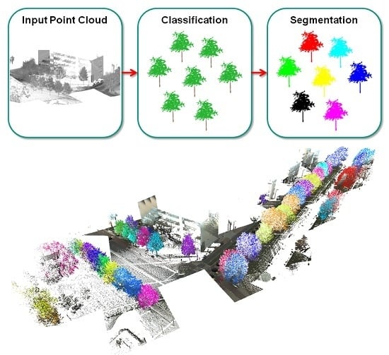
A Classification-Segmentation Framework for the Detection of Individual Trees in Dense MMS Point Cloud Data Acquired in Urban Areas


Abstract
:
1. Introduction
- feature subsets that are selected manually,
- feature subsets that are derived automatically via feature selection techniques and
- an improved segment-based shape analysis relying on semantic rules.
2. Related Work
2.1. Semantic Classification
2.2. Semantic Segmentation
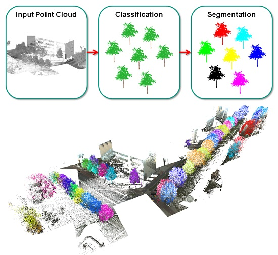
3. Methodology
3.1. Detection of Tree-Like Structures via Semantic Classification
3.1.1. Feature Extraction
3.1.2. Feature Selection
- The feature set contains the dimensionality features:
- The feature set contains the eight local 3D shape features:
- The feature set contains all defined 3D features, i.e., the local 3D shape features and the geometric 3D properties:
- The feature set contains all 3D and 2D features relying on the k-NN neighborhood, i.e., the local 3D shape features, the geometric 3D properties, the local 2D shape features and the geometric 2D properties:
- The feature set contains all 3D and 2D features as well as the given reflectance information:
- The feature set contains all defined 3D and 2D features as well as reflectance and color information:
3.1.3. Supervised Classification
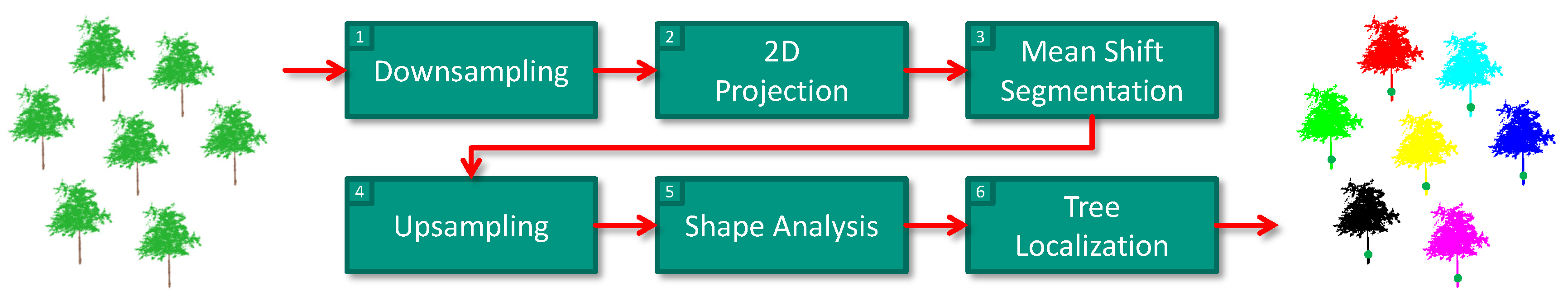
3.2. Separation of Individual Trees via Semantic Segmentation
3.2.1. Downsampling
3.2.2. 2D Projection
3.2.3. Mean Shift Segmentation
- calculation of the weighted mean μ of all data points within a window centered at and defined via a kernel (whereby the kernel is typically represented by an isotropic kernel such as a Gaussian kernel or an Epanechnikov kernel [81]),
- definition of the mean shift vector from the difference between and μ,
- movement of the data point along the mean shift vector and
- consideration of the resulting point as an update of the point .
3.2.4. Upsampling
3.2.5. Shape Analysis
- The first semantic rule focuses on discarding smaller segments comprising only relatively few 3D points. This is motivated by the fact that, due to the data acquisition with a mobile mapping system, the meaningful segments corresponding to individual trees should comprise many densely sampled 3D points, whereas small segments are not likely to correspond to the objects of interest, i.e., individual trees. Using a superscript to indicate segment-wise features, we apply this semantic rule to discard segments that comprise less than points.
- The second semantic rule focuses on failure cases observed in recent investigations, e.g., in the form of misclassifications of 3D points corresponding to building facades, which for instance becomes visible in the classification results for one of the approaches presented in [13]. In this regard, we take into account that building facades are characterized by an almost line-like structure in their 2D projection onto a horizontally oriented plane. Accordingly, we may consider the ratio of the eigenvalues of the 2D structure tensor, and we discard those segments that are rather elongated in the 2D projection by checking if is below a certain threshold . Thereby, we select the threshold heuristically to , which means that, for a segment corresponding to a tree, the smaller eigenvalue has to be equal to or even above a value of 20% of the larger eigenvalue , i.e., .
- The third semantic rule focuses on discarding segments that exhibit a structure with almost no extent in the horizontal direction. This can be done by thresholding the products of the eigenvalues of the 2D structure tensor and their sum , where we assume that segments corresponding to individual trees are characterized by m and m.
- The fourth semantic rule focuses on discarding segments that exhibit a low curvature where , since such segments typically reveal planar structures.
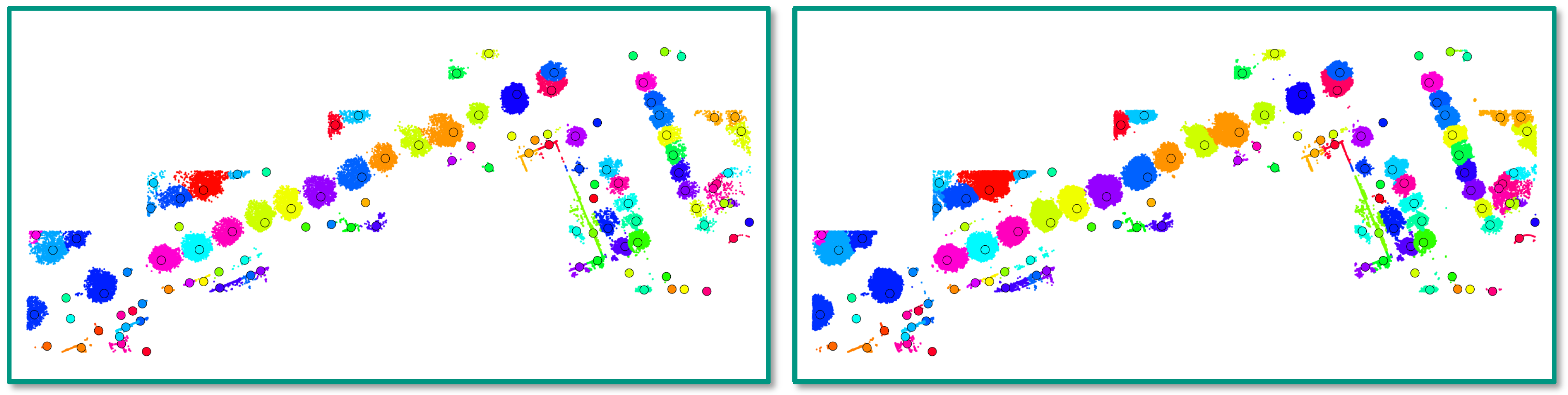
3.2.6. Tree Localization
4. Results
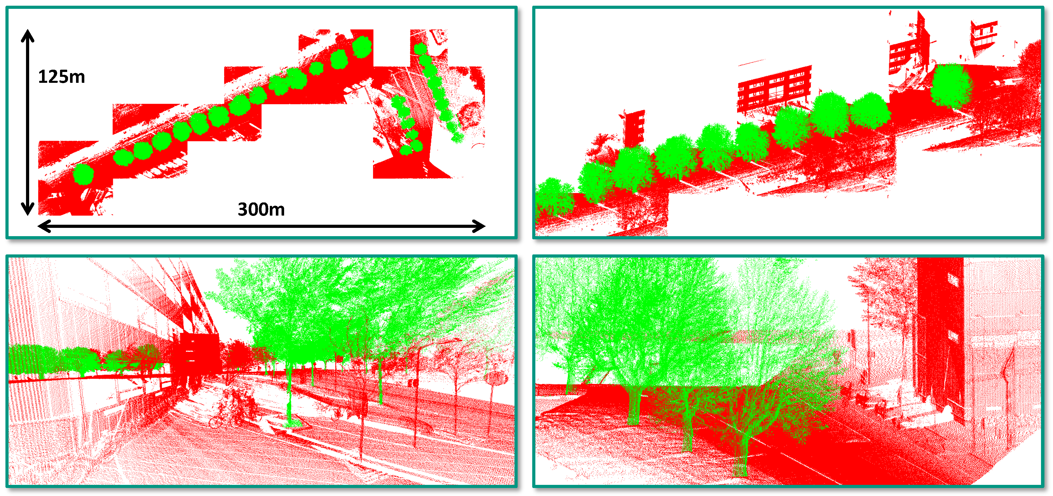
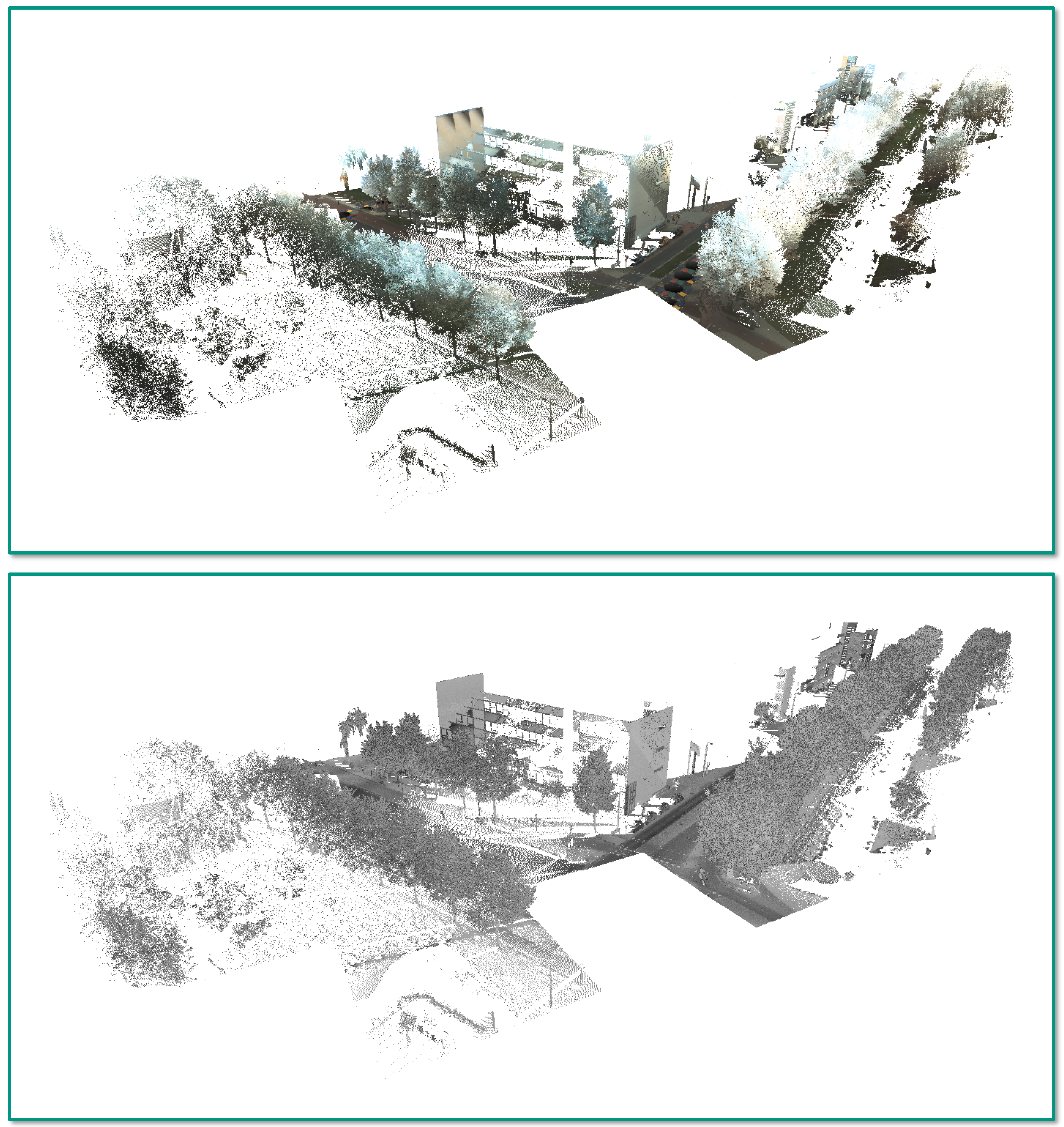
4.1. Dataset
4.2. Task 1: Semantic Classification
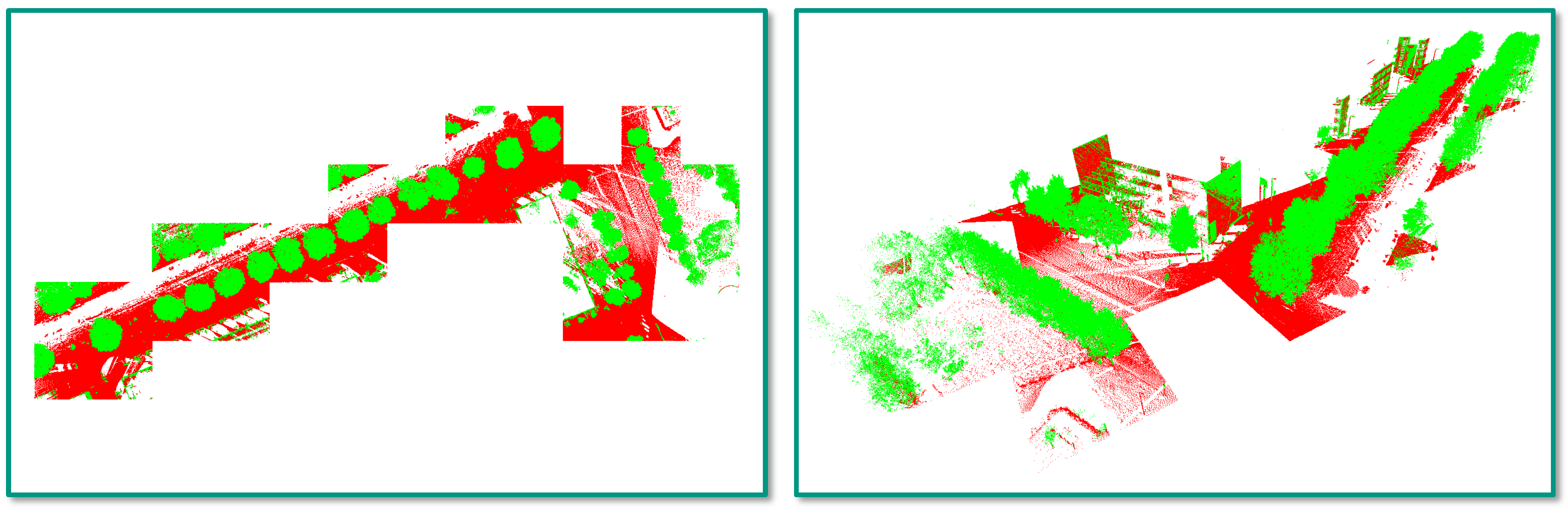
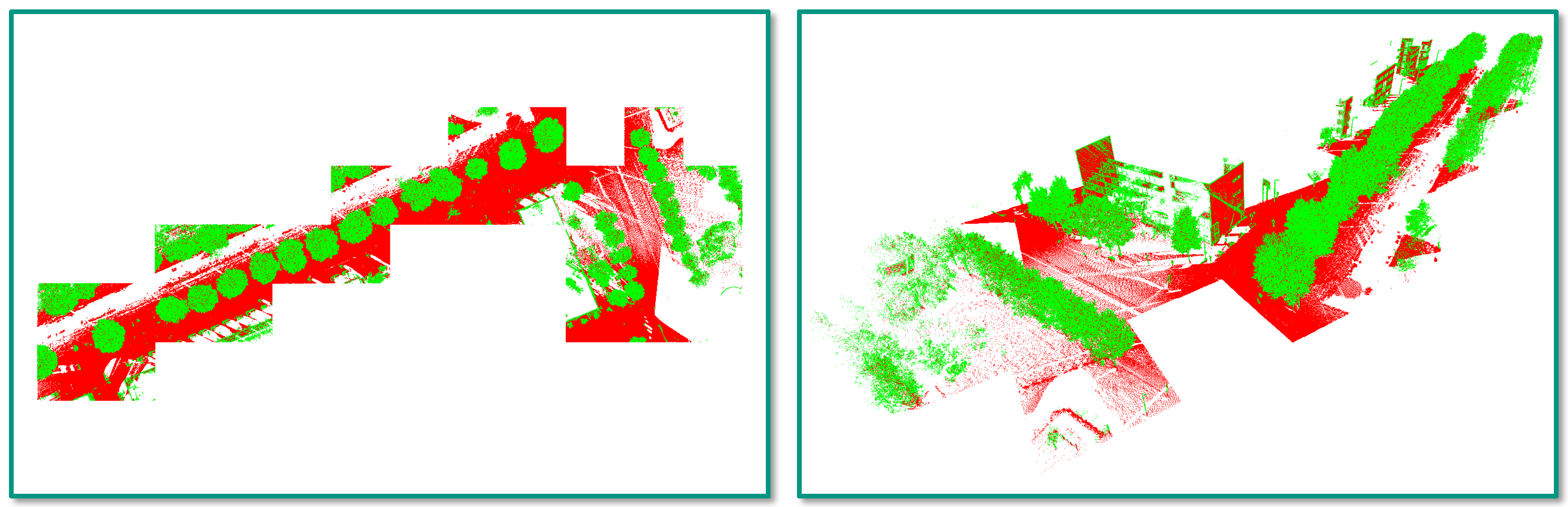
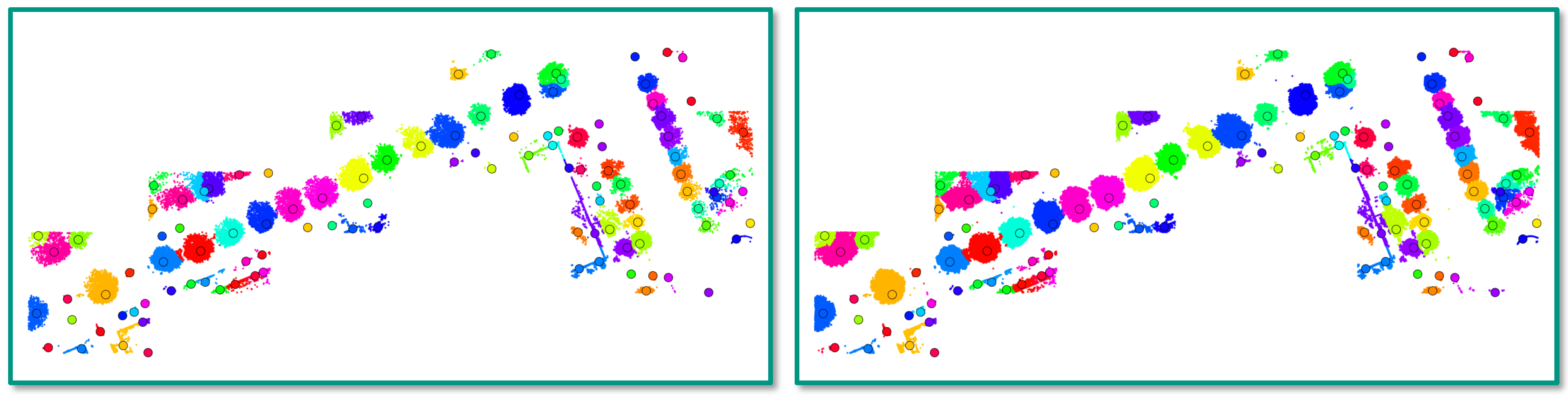
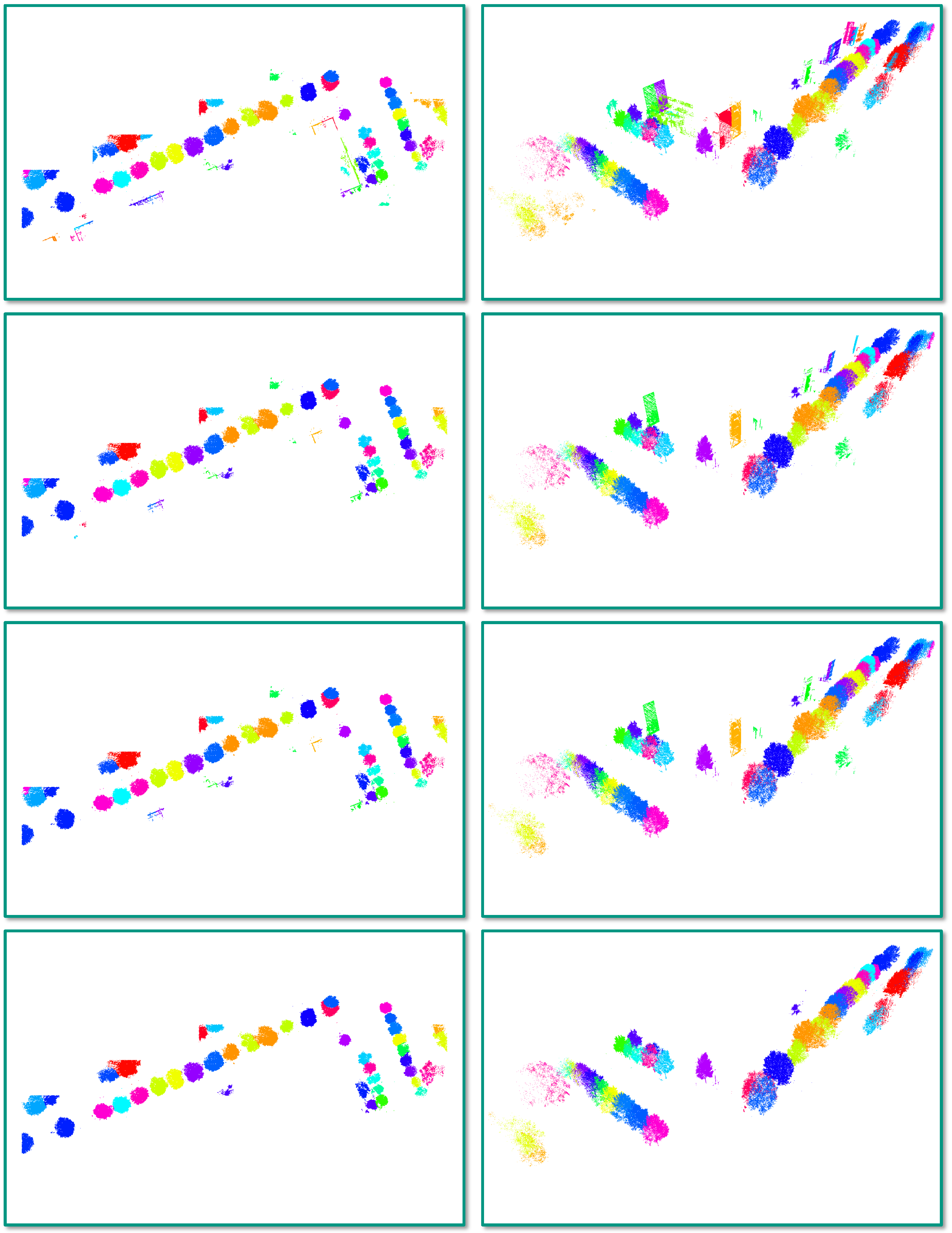
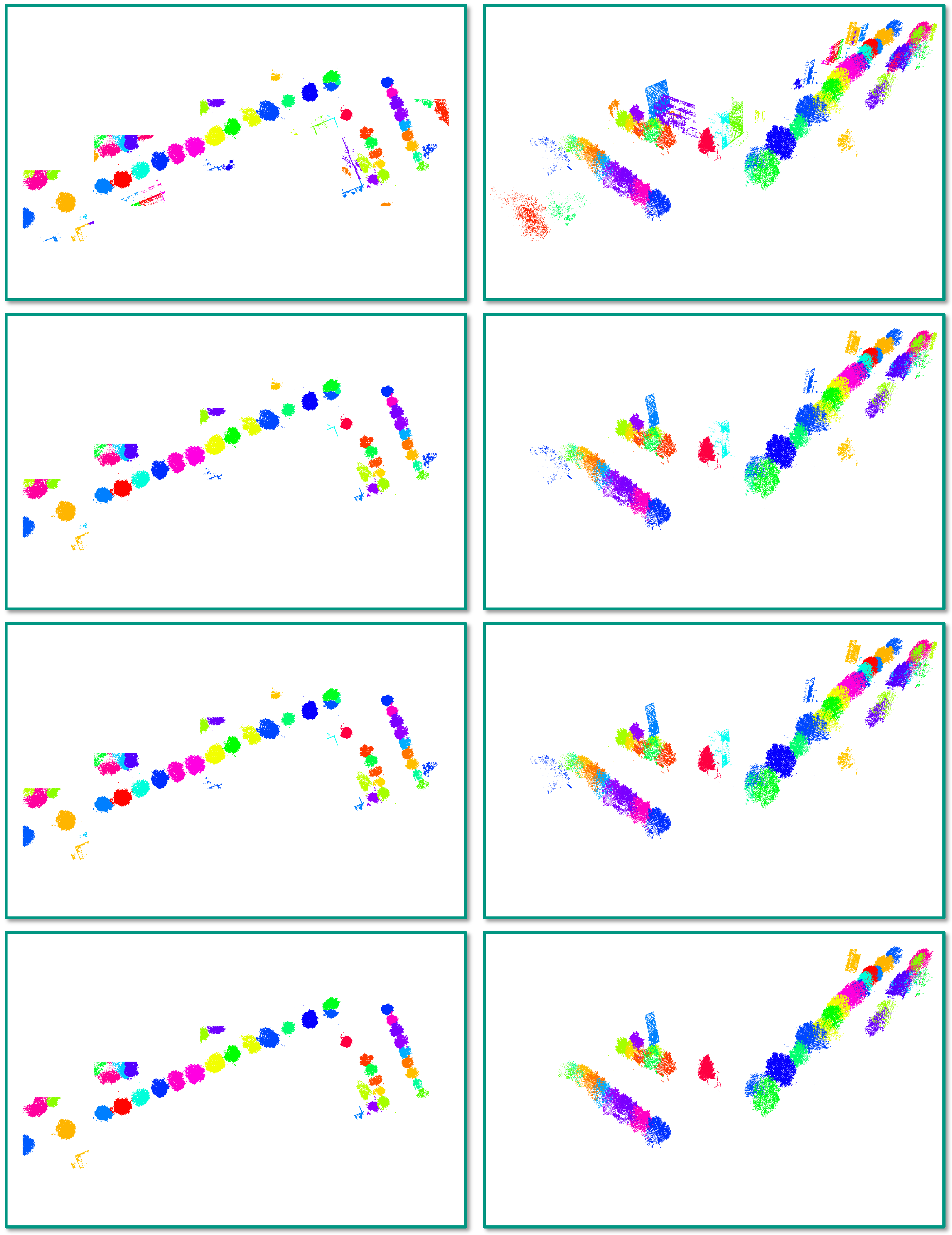
4.3. Task 2: Semantic Segmentation
5. Discussion
5.1. Task 1: Semantic Classification
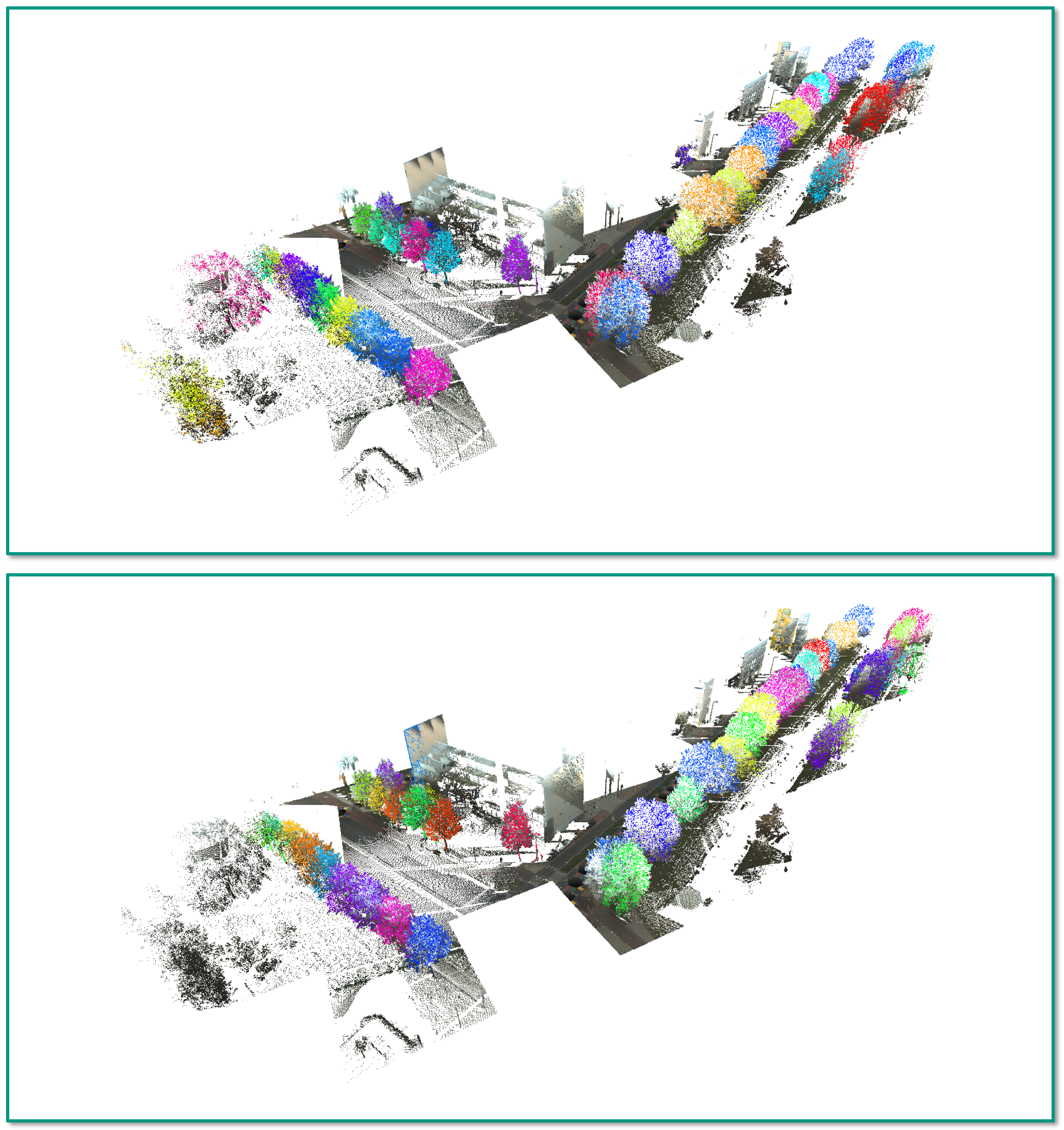
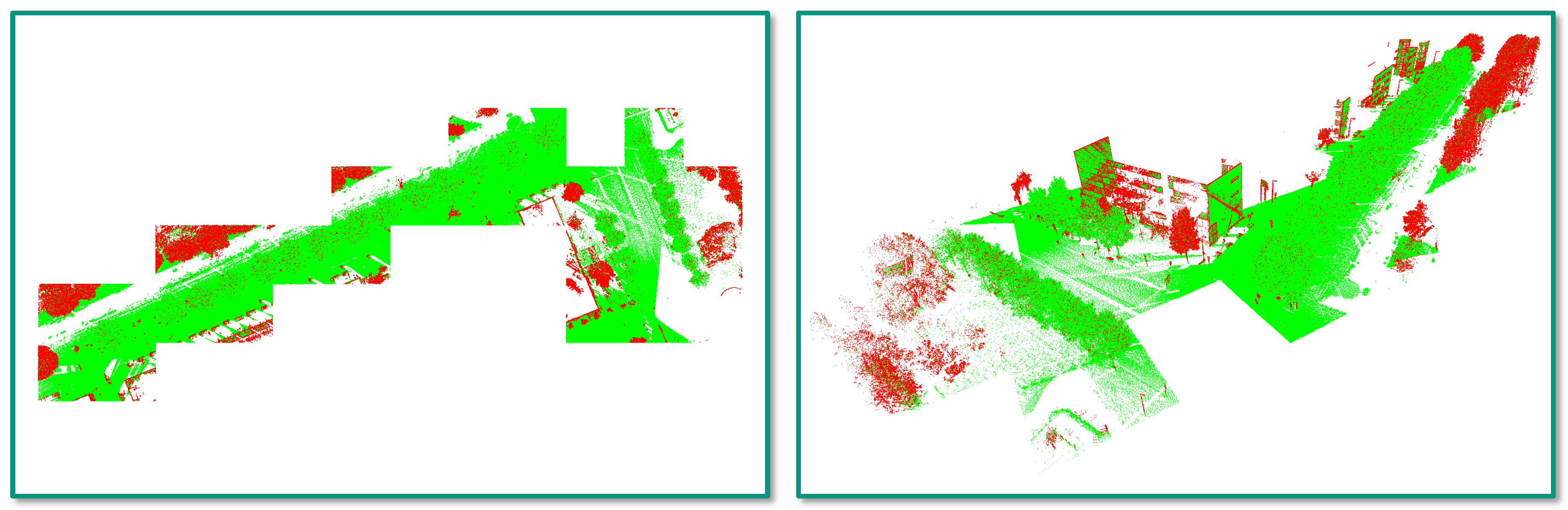
- Incorrect reference labels: A closer look at Figure 4 already reveals that some mislabeling obviously occurred during the annotation process. Some of the trees in the scene are completely labeled as “other points”, while the respective label should have been “tree points” instead. Due to the random sampling of training examples, some incorrectly labeled 3D points might have been selected for training the involved RF classifier, and hence, its generalization capability might be reduced. Furthermore, the incorrect labeling has a negative impact on the derived classification results as a significant number of correctly classified 3D points is considered as classification errors (Figure 12 and Figure 13).
- Registration errors: The visualization of the classified 3D point clouds in Figure 5 and Figure 6 as well as the visualization of failure cases in Figure 12 and Figure 13 reveal that certain 3D points corresponding to building facades are likely to be classified as “tree points”, although they should be labeled as “other points”. Such misclassifications might be caused by the fact that the local neighborhood of respective 3D points is characterized by a volumetric behavior instead of a planar behavior. The volumetric behavior in turn might result from a slight misalignment of different MMS point clouds or from a degraded positioning accuracy of the involved MMS system due to GNSS multipath errors, which are more significant in urban canyons. Furthermore, the volumetric behavior could result from noise effects resulting from limitations of the used sensor in terms of beam divergence or measurement accuracy, but also from specific characteristics of the observed scene in terms of object materials, surface reflectivity and surface roughness [22]. Besides these influencing factors, the scanning geometry in terms of the distance and orientation of object surfaces with respect to the used sensor might have to be considered as well [84,85].
- Edge effects: For some feature sets, misclassifications might occur at the boundaries of single tiles, which is due to the separate processing of different tiles [21]. This can easily be solved by considering a small padding region around each tile so that those 3D points within the padding region are also used if they are within the local neighborhood of a 3D point within the considered tile [5].
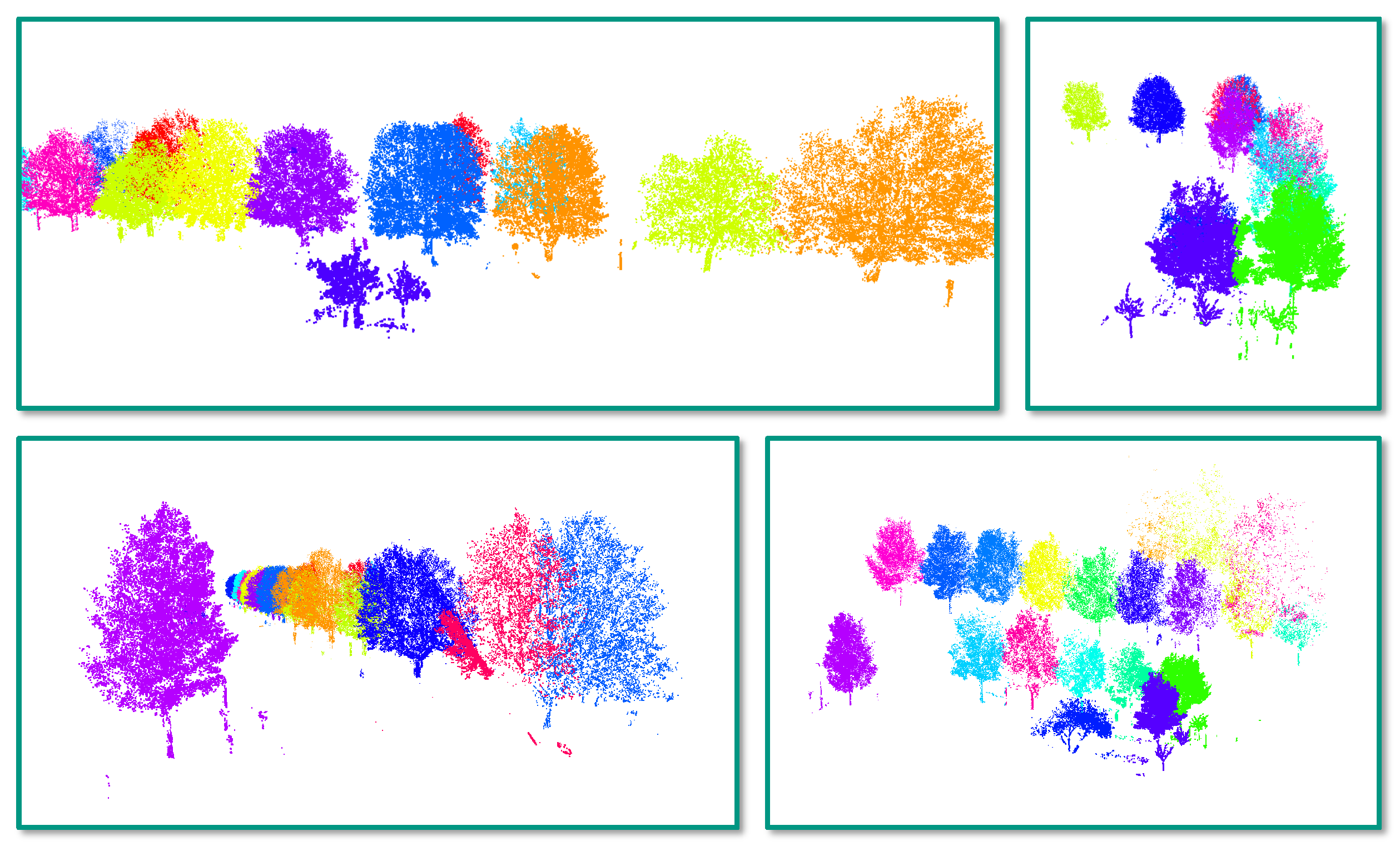
5.2. Task 2: Semantic Segmentation
5.3. Computational Effort
6. Conclusions
Acknowledgments
Author Contributions
Conflicts of Interest
References
- Munoz, D.; Bagnell, J.A.; Vandapel, N.; Hebert, M. Contextual classification with functional max-margin Markov networks. In Proceedings of the IEEE Conference on Computer Vision and Pattern Recognition, Miami, FL, USA, 20–25 June 2009; pp. 975–982.
- Xiong, X.; Munoz, D.; Bagnell, J.A.; Hebert, M. 3-D scene analysis via sequenced predictions over points and regions. In Proceedings of the IEEE International Conference on Robotics and Automation, Shanghai, China, 9–13 May 2011; pp. 2609–2616.
- Hu, H.; Munoz, D.; Bagnell, J.A.; Hebert, M. Efficient 3-D scene analysis from streaming data. In Proceedings of the IEEE International Conference on Robotics and Automation, Karlsruhe, Germany, 6–10 May 2013; pp. 2297–2304.
- Brédif, M.; Vallet, B.; Serna, A.; Marcotegui, B.; Paparoditis, N. TerraMobilita/IQmulus urban point cloud classification benchmark. In Proceedings of the IQmulus Workshop on Processing Large Geospatial Data, Cardiff, UK, 8 July 2014; pp. 1–6.
- Weinmann, M.; Urban, S.; Hinz, S.; Jutzi, B.; Mallet, C. Distinctive 2D and 3D features for automated large-scale scene analysis in urban areas. Comput. Graph. 2015, 49, 47–57. [Google Scholar] [CrossRef]
- Weinmann, M.; Jutzi, B.; Hinz, S.; Mallet, C. Semantic point cloud interpretation based on optimal neighborhoods, relevant features and efficient classifiers. ISPRS J. Photogramm. Remote Sens. 2015, 105, 286–304. [Google Scholar] [CrossRef]
- Hackel, T.; Wegner, J.D.; Schindler, K. Fast semantic segmentation of 3D point clouds with strongly varying density. ISPRS Ann. Photogramm. Remote Sens. Spat. Inf. Sci. 2016, III-3, 177–184. [Google Scholar] [CrossRef]
- Vanegas, C.A.; Aliaga, D.G.; Benes, B. Automatic extraction of Manhattan-world building masses from 3D laser range scans. IEEE Trans. Vis. Comput. Graph. 2012, 18, 1627–1637. [Google Scholar] [CrossRef] [PubMed]
- Boyko, A.; Funkhouser, T. Extracting roads from dense point clouds in large scale urban environment. ISPRS J. Photogramm. Remote Sens. 2011, 66, S02–S12. [Google Scholar] [CrossRef]
- Zhou, L.; Vosselman, G. Mapping curbstones in airborne and mobile laser scanning data. Int. J. Appl. Earth Observ. Geoinf. 2012, 18, 293–304. [Google Scholar] [CrossRef]
- Guan, H.; Li, J.; Yu, Y.; Wang, C.; Chapman, M.; Yang, B. Using mobile laser scanning data for automated extraction of road markings. ISPRS J. Photogramm. Remote Sens. 2014, 87, 93–107. [Google Scholar] [CrossRef]
- Pu, S.; Rutzinger, M.; Vosselman, G.; Oude Elberink, S. Recognizing basic structures from mobile laser scanning data for road inventory studies. ISPRS J. Photogramm. Remote Sens. 2011, 66, S28–S39. [Google Scholar] [CrossRef]
- Gorte, B.; Oude Elberink, S.; Sirmacek, B.; Wang, J. IQPC 2015 Track: Tree separation and classification in mobile mapping lidar data. Int. Arch. Photogramm. Remote Sens. Spat. Inf. Sci. 2015, XL-3/W3, 607–612. [Google Scholar] [CrossRef]
- Sirmacek, B.; Lindenbergh, R. Automatic classification of trees from laser scanning point clouds. ISPRS Ann. Photogramm. Remote Sens. Spat. Inf. Sci. 2015, II-3/W5, 137–144. [Google Scholar] [CrossRef]
- Lindenbergh, R.C.; Berthold, D.; Sirmacek, B.; Herrero-Huerta, M.; Wang, J.; Ebersbach, D. Automated large scale parameter extraction of road-side trees sampled by a laser mobile mapping system. Int. Arch. Photogramm. Remote Sens. Spat. Inf. Sci. 2015, XL-3/W3, 589–594. [Google Scholar] [CrossRef]
- Kelly, M. Urban trees and the green infrastructure agenda. In Proceedings of the Urban Trees Research Conference, Birmingham, UK, 13–14 April 2011; pp. 166–180.
- Edmondson, J.L.; Stott, I.; Davies, Z.G.; Gaston, K.J.; Leake, J.R. Soil surface temperatures reveal moderation of the urban heat island effect by trees and shrubs. Sci. Rep. 2016, 6, 1–8. [Google Scholar] [CrossRef] [Green Version]
- Wegner, J.D.; Branson, S.; Hall, D.; Schindler, K.; Perona, P. Cataloging public objects using aerial and street-level images – Urban trees. In Proceedings of the IEEE Conference on Computer Vision and Pattern Recognition, Las Vegas, NV, USA, 26 June–1 July 2016; pp. 6014–6023.
- Zhang, Z.; Fidler, S.; Urtasun, R. Instance-level segmentation for autonomous driving with deep densely connected MRFs. In Proceedings of the IEEE Conference on Computer Vision and Pattern Recognition, Las Vegas, NV, USA, 26 June–1 July 2016; pp. 669–677.
- Silberman, N.; Sontag, D.; Fergus, R. Instance segmentation of indoor scenes using a coverage loss. In Proceedings of the European Conference on Computer Vision, Zurich, Switzerland, 6–12 September 2014; pp. 616–631.
- Weinmann, M.; Mallet, C.; Brédif, M. Detection, segmentation and localization of individual trees from MMS point cloud data. In Proceedings of the International Conference on Geographic Object-Based Image Analysis, Enschede, The Netherlands, 14–16 September 2016; pp. 1–8.
- Weinmann, M. Reconstruction and Analysis of 3D Scenes—From Irregularly Distributed 3D Points to Object Classes; Springer: Cham, Switzerland, 2016. [Google Scholar]
- Melzer, T. Non-parametric segmentation of ALS point clouds using mean shift. J. Appl. Geod. 2007, 1, 159–170. [Google Scholar] [CrossRef]
- Vosselman, G. Point cloud segmentation for urban scene classification. Int. Arch. Photogramm. Remote Sens. Spat. Inf. Sci. 2013, XL-7/W2, 257–262. [Google Scholar] [CrossRef]
- Lee, I.; Schenk, T. Perceptual organization of 3D surface points. Int. Arch. Photogramm. Remote Sens. Spat. Inf. Sci. 2002, XXXIV-3A, 193–198. [Google Scholar]
- Linsen, L.; Prautzsch, H. Local versus global triangulations. In Proceedings of Eurographics, Manchester, UK, 5–7 September 2001; pp. 257–263.
- Filin, S.; Pfeifer, N. Neighborhood systems for airborne laser data. Photogramm. Eng. Remote Sens. 2005, 71, 743–755. [Google Scholar] [CrossRef]
- Pauly, M.; Keiser, R.; Gross, M. Multi-scale feature extraction on point-sampled surfaces. Comput. Graph. Forum 2003, 22, 81–89. [Google Scholar] [CrossRef]
- Mitra, N.J.; Nguyen, A. Estimating surface normals in noisy point cloud data. In Proceedings of the Annual Symposium on Computational Geometry, San Diego, CA, USA, 8–10 June 2003; pp. 322–328.
- Lalonde, J.F.; Unnikrishnan, R.; Vandapel, N.; Hebert, M. Scale selection for classification of point-sampled 3D surfaces. In Proceedings of the International Conference on 3-D Digital Imaging and Modeling, Ottawa, ON, Canada, 13–16 June 2005; pp. 285–292.
- Demantké, J.; Mallet, C.; David, N.; Vallet, B. Dimensionality based scale selection in 3D lidar point clouds. Int. Arch. Photogramm. Remote Sens. Spat. Inf. Sci. 2011, XXXVIII-5/W12, 97–102. [Google Scholar] [CrossRef]
- Brodu, N.; Lague, D. 3D terrestrial lidar data classification of complex natural scenes using a multi-scale dimensionality criterion: Applications in geomorphology. ISPRS J. Photogramm. Remote Sens. 2012, 68, 121–134. [Google Scholar] [CrossRef] [Green Version]
- Niemeyer, J.; Rottensteiner, F.; Soergel, U. Contextual classification of lidar data and building object detection in urban areas. ISPRS J. Photogramm. Remote Sens. 2014, 87, 152–165. [Google Scholar] [CrossRef]
- Blomley, R.; Jutzi, B.; Weinmann, M. Classification of airborne laser scanning data using geometric multi-scale features and different neighbourhood types. ISPRS Ann. Photogramm. Remote Sens. Spat. Inf. Sci. 2016, III-3, 169–176. [Google Scholar] [CrossRef]
- Gevaert, C.M.; Persello, C.; Vosselman, G. Optimizing multiple kernel learning for the classification of UAV data. Remote Sens. 2016, 8, 1025. [Google Scholar] [CrossRef]
- West, K.F.; Webb, B.N.; Lersch, J.R.; Pothier, S.; Triscari, J.M.; Iverson, A.E. Context-driven automated target detection in 3-D data. Proc. SPIE 2004, 5426, 133–143. [Google Scholar]
- Mallet, C.; Bretar, F.; Roux, M.; Soergel, U.; Heipke, C. Relevance assessment of full-waveform lidar data for urban area classification. ISPRS J. Photogramm. Remote Sens. 2011, 66, S71–S84. [Google Scholar] [CrossRef]
- Guo, B.; Huang, X.; Zhang, F.; Sohn, G. Classification of airborne laser scanning data using JointBoost. ISPRS J. Photogramm. Remote Sens. 2015, 100, 71–83. [Google Scholar] [CrossRef]
- Hughes, G.F. On the mean accuracy of statistical pattern recognizers. IEEE Trans. Inf. Theory 1968, 14, 55–63. [Google Scholar] [CrossRef]
- Weinmann, M.; Jutzi, B.; Mallet, C. Feature relevance assessment for the semantic interpretation of 3D point cloud data. ISPRS Ann. Photogramm. Remote Sens. Spat. Inf. Sci. 2013, II-5/W2, 313–318. [Google Scholar] [CrossRef]
- Khoshelham, K.; Oude Elberink, S.J. Role of dimensionality reduction in segment-based classification of damaged building roofs in airborne laser scanning data. In Proceedings of the International Conference on Geographic Object Based Image Analysis, Rio de Janeiro, Brazil, 7–9 May 2012; pp. 372–377.
- Schindler, K. An overview and comparison of smooth labeling methods for land-cover classification. IEEE Trans. Geosci. Remote Sens. 2012, 50, 4534–4545. [Google Scholar] [CrossRef]
- Shapovalov, R.; Velizhev, A.; Barinova, O. Non-associative Markov networks for 3D point cloud classification. Int. Arch. Photogramm. Remote Sens. Spat. Inf. Sci. 2010, XXXVIII-3A, 103–108. [Google Scholar]
- Niemeyer, J.; Rottensteiner, F.; Soergel, U. Conditional random fields for lidar point cloud classification in complex urban areas. ISPRS Ann. Photogramm. Remote Sens. Spat. Inf. Sci. 2012, I-3, 263–268. [Google Scholar] [CrossRef]
- Schmidt, A.; Niemeyer, J.; Rottensteiner, F.; Soergel, U. Contextual classification of full waveform lidar data in the Wadden Sea. IEEE Geosci. Remote Sens. Lett. 2014, 11, 1614–1618. [Google Scholar] [CrossRef]
- Weinmann, M.; Schmidt, A.; Mallet, C.; Hinz, S.; Rottensteiner, F.; Jutzi, B. Contextual classification of point cloud data by exploiting individual 3D neighborhoods. ISPRS Ann. Photogramm. Remote Sens. Spat. Inf. Sci. 2015, II-3/W4, 271–278. [Google Scholar] [CrossRef]
- Shapovalov, R.; Vetrov, D.; Kohli, P. Spatial inference machines. In Proceedings of the IEEE Conference on Computer Vision and Pattern Recognition, Portland, OR, USA, 23–28 June 2013; pp. 2985–2992.
- Maturana, D.; Scherer, S. VoxNet: A 3D convolutional neural network for real-time object recognition. In Proceedings of the IEEE/RSJ International Conference on Intelligent Robots and Systems, Hamburg, Germany, 28 September–2 October 2015; pp. 922–928.
- Wu, Z.; Song, S.; Khosla, A.; Yu, F.; Zhang, L.; Tang, X.; Xiao, J. 3D ShapeNets: A deep representation for volumetric shapes. In Proceedings of the IEEE Conference on Computer Vision and Pattern Recognition, Boston, MA, USA, 7–12 June 2015; pp. 1912–1920.
- Riegler, G.; Ulusoy, A.O.; Geiger, A. OctNet: Learning deep 3D representations at high resolutions. arXiv 2017. [Google Scholar]
- Savinov, N. Point Cloud Semantic Segmentation via Deep 3D Convolutional Neural Network. 2017. Available online: https://github.com/nsavinov/semantic3dnet (accessed on 6 March 2017).
- Huang, J.; You, S. Point cloud labeling using 3D convolutional neural network. In Proceedings of the International Conference on Pattern Recognition, Cancun, Mexico, 4–8 December 2016; pp. 1–6.
- Large-Scale Point Cloud Classification Benchmark. 2016. Available online: http://www.semantic3d.net (accessed on 6 March 2017).
- Serna, A.; Marcotegui, B.; Goulette, F.; Deschaud, J.E. Paris-rue-Madame database: A 3D mobile laser scanner dataset for benchmarking urban detection, segmentation and classification methods. In Proceedings of the International Conference on Pattern Recognition Applications and Methods, Angers, France, 6–8 March 2014; pp. 819–824.
- Breiman, L. Random forests. Mach. Learn. 2001, 45, 5–32. [Google Scholar] [CrossRef]
- Zhang, J.; Lin, X.; Ning, X. SVM-based classification of segmented airborne lidar point clouds in urban areas. Remote Sens. 2013, 5, 3749–3775. [Google Scholar] [CrossRef]
- Aijazi, A.K.; Checchin, P.; Trassoudaine, L. Segmentation based classification of 3D urban point clouds: A super-voxel based approach with evaluation. Remote Sens. 2013, 5, 1624–1650. [Google Scholar] [CrossRef]
- Wu, B.; Yu, B.; Yue, W.; Shu, S.; Tan, W.; Hu, C.; Huang, Y.; Wu, J.; Liu, H. A voxel-based method for automated identification and morphological parameters estimation of individual street trees from mobile laser scanning data. Remote Sens. 2013, 5, 584–611. [Google Scholar] [CrossRef]
- Yao, W.; Fan, H. Automated detection of 3D individual trees along urban road corridors by mobile laser scanning systems. In Proceedings of the International Symposium on Mobile Mapping Technology, Tainan, Taiwan, 1–3 May 2013; pp. 1–6.
- Reitberger, J.; Schnörr, C.; Krzystek, P.; Stilla, U. 3D segmentation of single trees exploiting full waveform lidar data. ISPRS J. Photogramm. Remote Sens. 2009, 64, 561–574. [Google Scholar] [CrossRef]
- Rutzinger, M.; Pratihast, A.K.; Oude Elberink, S.; Vosselman, G. Detection and modelling of 3D trees from mobile laser scanning data. Int. Arch. Photogramm. Remote Sens. Spat. Inf. Sci. 2010, XXXVIII-5, 520–525. [Google Scholar]
- Rutzinger, M.; Pratihast, A.K.; Oude Elberink, S.J.; Vosselman, G. Tree modelling from mobile laser scanning data-sets. Photogramm. Rec. 2011, 26, 361–372. [Google Scholar] [CrossRef]
- Monnier, F.; Vallet, B.; Soheilian, B. Trees detection from laser point clouds acquired in dense urban areas by a mobile mapping system. ISPRS Ann. Photogramm. Remote Sens. Spat. Inf. Sci. 2012, I-3, 245–250. [Google Scholar] [CrossRef]
- Oude Elberink, S.; Kemboi, B. User-assisted object detection by segment based similarity measures in mobile laser scanner data. Int. Arch. Photogramm. Remote Sens. Spat. Inf. Sci. 2014, XL-3, 239–246. [Google Scholar] [CrossRef]
- Gupta, S.; Weinacker, H.; Koch, B. Comparative analysis of clustering-based approaches for 3-D single tree detection using airborne fullwave lidar data. Remote Sens. 2010, 2, 968–989. [Google Scholar] [CrossRef]
- Fukunaga, K.; Hostetler, L. The estimation of the gradient of a density function, with applications in pattern recognition. IEEE Trans. Inf. Theory 1975, 21, 32–40. [Google Scholar] [CrossRef]
- Ferraz, A.; Bretar, F.; Jacquemoud, S.; Goncalves, G.; Pereira, L.; Tomé, M.; Soares, P. 3-D mapping of a multi-layered Mediterranean forest using ALS data. Remote Sens. Environ. 2012, 121, 210–223. [Google Scholar] [CrossRef]
- Schmitt, M.; Brück, A.; Schönberger, J.; Stilla, U. Potential of airborne single-pass millimeterwave InSAR data for individual tree recognition. In Proceedings of the Tagungsband der Dreiländertagung der DGPF, der OVG und der SGPF, Freiburg, Germany, 27 February–1 March 2013; Volume 22, pp. 427–436.
- Yao, W.; Krzystek, P.; Heurich, M. Enhanced detection of 3D individual trees in forested areas using airborne full-waveform lidar data by combining normalized cuts with spatial density clustering. ISPRS Ann. Photogramm. Remote Sens. Spat. Inf. Sci. 2013, II-5/W2, 349–354. [Google Scholar] [CrossRef]
- Shahzad, M.; Schmitt, M.; Zhu, X.X. Segmentation and crown parameter extraction of individual trees in an airborne TomoSAR point cloud. Int. Arch. Photogramm. Remote Sens. Spat. Inf. Sci. 2015, XL-3/W2, 205–209. [Google Scholar] [CrossRef]
- Schmitt, M.; Shahzad, M.; Zhu, X.X. Reconstruction of individual trees from multi-aspect TomoSAR data. Remote Sens. Environ. 2015, 165, 175–185. [Google Scholar] [CrossRef]
- Zhao, Z.; Morstatter, F.; Sharma, S.; Alelyani, S.; Anand, A.; Liu, H. Advancing Feature Selection Research — ASU Feature Selection Repository; Technical Report; School of Computing, Informatics, and Decision Systems Engineering, Arizona State University: Tempe, AZ, USA, 2010. [Google Scholar]
- Hall, M.A. Correlation-based feature subset selection for machine learning. Ph.D. thesis, Department of Computer Science, University of Waikato, Hamilton, New Zealand, 1999. [Google Scholar]
- Press, W.H.; Flannery, B.P.; Teukolsky, S.A.; Vetterling, W.T. Numerical recipes in C; Cambridge University Press: Cambridge, UK, 1988. [Google Scholar]
- Yu, L.; Liu, H. Feature selection for high-dimensional data: A fast correlation-based filter solution. In Proceedings of the International Conference on Machine Learning, Washington, DC, USA, 21–24 August 2003; pp. 856–863.
- Breiman, L. Bagging predictors. Mach. Learn. 1996, 24, 123–140. [Google Scholar] [CrossRef]
- Criminisi, A.; Shotton, J. Decision Forests for Computer Vision and Medical Image Analysis; Springer: London, UK, 2013. [Google Scholar]
- Weinmann, M.; Mallet, C.; Brédif, M. Segmentation and localization of individual trees from MMS point cloud data acquired in urban areas. In Proceedings of the Tagungsband der Dreiländertagung der DGPF, der OVG und der SGPF, Bern, Switzerland, 7–9 June 2016; Volume 25, pp. 351–360.
- Caraffa, L.; Brédif, M.; Vallet, B. 3D octree based watertight mesh generation from ubiquitous data. Int. Arch. Photogramm. Remote Sens. Spat. Inf. Sci. 2015, XL-3/W3, 613–617. [Google Scholar] [CrossRef]
- Cheng, Y. Mean shift, mode seeking, and clustering. IEEE Trans. Pattern Anal. Mach. Intell. 1995, 17, 790–799. [Google Scholar] [CrossRef]
- Comaniciu, D.; Meer, P. Mean shift: A robust approach toward feature space analysis. IEEE Trans. Pattern Anal. Mach. Intell. 2002, 24, 603–619. [Google Scholar] [CrossRef]
- Chen, C.; Liaw, A.; Breiman, L. Using Random Forest to Learn Imbalanced Data; Technical Report; University of California: Berkeley, CA, USA, 2004. [Google Scholar]
- Guyon, I.; Elisseeff, A. An introduction to variable and feature selection. J. Mach. Learn. Res. 2003, 3, 1157–1182. [Google Scholar]
- Soudarissanane, S.; Lindenbergh, R.; Menenti, M.; Teunissen, P. Scanning geometry: Influencing factor on the quality of terrestrial laser scanning points. ISPRS J. Photogramm. Remote Sens. 2011, 66, 389–399. [Google Scholar] [CrossRef]
- Weinmann, M.; Jutzi, B. Geometric point quality assessment for the automated, markerless and robust registration of unordered TLS point clouds. ISPRS Ann. Photogramm. Remote Sens. Spat. Inf. Sci. 2015, II-3/W5, 89–96. [Google Scholar] [CrossRef]
- Böhm, J.; Brédif, M.; Gierlinger, T.; Krämer, M.; Lindenbergh, R.; Liu, K.; Michel, F.; Sirmacek, B. The IQmulus urban showcase: Automatic tree classification and identification in huge mobile mapping point clouds. Int. Arch. Photogramm. Remote Sens. Spat. Inf. Sci. 2016, XLI-B3, 301–307. [Google Scholar]
- Wang, S.; Bai, M.; Mattyus, G.; Chu, H.; Luo, W.; Yang, B.; Liang, J.; Cheverie, J.; Fidler, S.; Urtasun, R. TorontoCity: Seeing the world with a million eyes. arXiv 2016. [Google Scholar]


| Feature | Formulae |
|---|---|
| Linearity | |
| Planarity | |
| Sphericity | |
| Omnivariance | |
| Anisotropy | |
| Eigenentropy | |
| Sum of eigenvalues | |
| Local surface variation | |
| Height | |
| Radius | |
| Local point density | |
| Verticality | |
| Height difference | |
| Standard deviation of height values |
| Feature Set | # Features | OA (%) | κ (%) | (%) | (%) | (%) | (%) |
|---|---|---|---|---|---|---|---|
| 3 | |||||||
| 8 | |||||||
| 14 | |||||||
| 18 | |||||||
| 19 | |||||||
| 22 | |||||||
| Specifications | Prototype [21] | Proposed Framework |
|---|---|---|
| System | Intel Core i7-3820, GHz, 64 GB RAM | Intel Core i7-6820HK, GHz, 16 GB RAM |
| Implementation | MATLAB | MATLAB |
| Parallelization | – | 4 cores |
| # Geometric Features | 21 | 18 |
| h | h | |
| h | h | |
| s | s | |
| s | s |
© 2017 by the authors. Licensee MDPI, Basel, Switzerland. This article is an open access article distributed under the terms and conditions of the Creative Commons Attribution (CC BY) license ( http://creativecommons.org/licenses/by/4.0/).
Share and Cite
Weinmann, M.; Weinmann, M.; Mallet, C.; Brédif, M. A Classification-Segmentation Framework for the Detection of Individual Trees in Dense MMS Point Cloud Data Acquired in Urban Areas. Remote Sens. 2017, 9, 277. https://doi.org/10.3390/rs9030277
Weinmann M, Weinmann M, Mallet C, Brédif M. A Classification-Segmentation Framework for the Detection of Individual Trees in Dense MMS Point Cloud Data Acquired in Urban Areas. Remote Sensing. 2017; 9(3):277. https://doi.org/10.3390/rs9030277
Chicago/Turabian StyleWeinmann, Martin, Michael Weinmann, Clément Mallet, and Mathieu Brédif. 2017. "A Classification-Segmentation Framework for the Detection of Individual Trees in Dense MMS Point Cloud Data Acquired in Urban Areas" Remote Sensing 9, no. 3: 277. https://doi.org/10.3390/rs9030277