Article

Three-Step Semi-Empirical Radiometric Terrain Correction Approach for PolSAR Data Applied to Forested Areas

1
Institute of Forest Resources Information Technique, Chinese Academy of Forestry, Beijing 100091, China
2
College of Forestry, Southwest Forestry University, Kunming 650224, China
*
Author to whom correspondence should be addressed.
Remote Sens. 2017, 9(3), 269; https://doi.org/10.3390/rs9030269
Submission received: 14 October 2016 / Revised: 23 February 2017 / Accepted: 12 March 2017 / Published: 15 March 2017

Abstract

:
In recent decades, most methods proposed for radiometric slope correction involved the backscattering intensity values in synthetic aperture radar (SAR) data. However, these methods are not fully applicable to quad-polarimetric SAR (PolSAR) matrix data. In this paper, we propose a three-step semi-empirical radiometric terrain correction approach for PolSAR forest area data. The three steps of terrain effects correction are: polarisation orientation angle (POA), effective scattering area (ESA), and angular variation effect (AVE) corrections. We propose a novel method to determine adaptively the “n” value in the third step by minimising the correlation coefficient between corrected backscattering coefficients and the local incidence angle; we then constructed the correction coefficients matrix and used it to correct PolSAR matrix data. PALSAR-2 HBQ (L-band, quad-polarisation) data were used to verify the proposed method. After three-step correction, differences between front and back slopes were significantly reduced. Our results indicate that POA, ESA, and AVE corrections are indispensable steps to producing PolSAR data. In the POA correction step, horizontal–vertical (HV) polarisation was maximally influenced by the POA shift. The max deviation of the POA correction was greater than 1 dB for HV polarisation and approximately 0.5 dB for HH/VV polarisation at an intermediate shift angle (±20°). Based on Light Detection and Ranging (LiDAR)-derived forest aboveground biomass (AGB) data, we analysed the relationship between forest AGB and backscattering coefficient; the correlation was improved following the terrain correction. HV polarisation had the best correlation with forest AGB (R = 0.81) and the correlation improved by approximately 0.3 compared to the uncorrected data.

Graphical Abstract

1. Introduction

Full polarimetric synthetic aperture radar (PolSAR), a recently developed, advanced remote sensing technology, has been widely used in the field of earth observation. Because PolSAR combines the merits of microwave penetration and polarisation measurement, it has advantages in the estimation of forest traits, such as forest aboveground biomass (AGB). However, its application is greatly limited by the terrain. Owing to the characteristics of side-looking illumination by SAR sensors, terrain undulations seriously affect the radiometric quality of SAR images. The correction of these effects becomes crucial when quantitative analysis is performed with respect to the derivation of geo- and biophysical parameters [1]. This correction is typically referred to as Radiometric Terrain Correction (RTC) [2]. For single- or dual-polarisation SAR, the object of RTC is a backscattering coefficient value for different polarisations, such as σHH, σHV or σVV. However, for PolSAR, the object of RTC is a polarisation scattering matrix, such as the Sinclair matrix (S), polarisation covariance matrix (C) or polarisation coherency matrix (T). Compared to single- or dual-polarisation SAR, the influence of topography for PolSAR is more complex.
For SAR data, the effect of terrain can be summarised in three aspects. The first is variation in the effective scattering area (ESA), which depends on the local imaging geometry. For example, on the front slope, one pixel in an SAR image corresponds to more ground area than it would on the back slope. The second is variation in scattering mechanisms and penetration depth, among others. These phenomena are collectively known as the angular variation effect (AVE), which mainly appears in areas of vegetation [3,4]. The third is variation in polarisation states, caused by azimuth slopes, which induces polarisation orientation angle (POA) changes [5]. This effect occurs only in PolSAR data.
ESA correction requires accurate description of the SAR imaging geometry based on the topological relationship between slant range radar coordinates and the map grid of local topography. Several studies have been published on this topic. The methods are based on local incidence angle [6], surface tilt angle [2,7], projection angle [8], and area integral [9,10]; the most accurate of these are the projection angle and area integral methods. The topological relationship used in these methods may be divided into two types: homomorphic [2,6,7,8] and heteromorphic [9,10], as proposed by Small [9,11]. It has been shown that homomorphism is not an appropriate assumption, compared to heteromorphism [9,11]. However, the prerequisite for heteromorphism is high-resolution Digital Elevation Model (DEM) data, which must have resolution equal to or better than that of the SAR data [9].
Among the three terrain correction steps, ESA correction is the most fundamental. In the case of single- or dual-polarisation SAR and over areas not covered by vegetation, ESA correction is sufficient. However, for areas with vegetation coverage, it is necessary to perform further AVE correction through a basic model using the nth power of the cosine of the local incident angle [12]. The key problem lies in determining the value of n, which depends on the terrain cover type, radar frequency, and polarisation mode. Castel et al. [3] proposed a semi-empirical model to determine the value of n based on radiative transfer theory, which has a single parameter describing the canopy optical thinness. Sun et al. [13] adopted a three-dimensional (3D) radar backscatter model to simulate a series of SAR images for one forest scene with various surface slopes. The value of n was acquired by analysing the variation rule of the simulated backscattering values. However, these two methods are ordinarily too difficult to perform because both require a priori knowledge. Therefore, the objective of the current study is to find a more automated method to determine the value of n.
As mentioned above, the two correction processes are typically sufficient for single- or dual-polarisation SAR data. However, for PolSAR data, POA correction is also required. Related theories were first raised by Lee and Schuler [5], who proposed using the classic circular polarisation method to calculate the shift angle of POA; the shift angle may be used to compensate for the azimuth slope effect in PolSAR data. Villard et al. [4] proposed a new numerical method to calculate the POA shift angle from a polarisation coherency matrix. The difference is that circular polarisation method nullifies the real part of T23 (2nd row, 3rd column element of T), whereas the numerical method of Villard aims at cancelling the complex terms T13 (1st row, 3rd column element of T) and T23 through a quadratic positive cost function [4]. Kobayashi et al. found that the correlation between industrial plantation forest parameters and decomposition parameters in PolSAR data improved following the POA correction process [14].
Currently, SAR data terrain correction methods are mainly a combination of the three correction types. For example, Castel et al. [3], Sun et al. [13], and Hoekman et al. [15] combined the ESA and AVE corrections to handle the terrain effects for single- or dual-polarisation SAR data in forest-covered areas. Wang et al. proposed an improved PolSAR RTC method combining ESA and POA correction methods; improved results were obtained when they applied their approaches to PolSAR data for land cover classification [16]. In a study of forest AGB retrieval using P-band PolSAR data, Villard et al. adopted the ESA, AVE, and POA correction methods to develop a new backscattering coefficient called t0 that yields a better correlation with forest AGB [4]. However, in their AVE correction procedure, the value of n was also determined according to expertise.
In summary, the general consensus is that a single correction method is insufficient to handle topography effects in PolSAR data. A comprehensive and systematic RTC method is urgently needed to treat PolSAR data. Furthermore, the correction should be changed from a single backscattering coefficient to a full polarisation scattering matrix. The overall correction process should be more automated to facilitate practical application. Nevertheless, such practical approaches have not yet been developed.
In this study, we propose a novel approach to determine the value of n in AVE correction adaptively. By integrating the AVE correction method into the entire correction process, we developed a three-step terrain correction method for PolSAR data. The three-step method, specially developed for PolSAR matrix data, is comprehensive, convenient, and efficient, requiring less prior knowledge. In addition to the proposed method, which includes the POA, ESA, and AVE correction methods, we present a demonstration and analysis of the method as applied to a forested area using ALOS-2 PALSAR-2 PolSAR data.

2. Methods

2.1. Framework of the Proposed Method

The processing flow chart presented in Figure 1 provides details of the proposed method, which includes three key data processing steps. In PolSAR data pre-processing, single-look complex (SLC) PolSAR data must be calibrated, multi-looked, or filtered. Next, geocoding of terrain correction (GTC) is performed. In satellite SAR, the geocoding process is completed based on precise satellite orbit information and DEM data using a Range Doppler (RD) position model. This is an indispensable step in the SAR RTC process [1]. Then, we obtain the mapping relationship (GTC model) between SAR slant-range space and geographic space, and local imaging geometry information that is also required for ESA and AVE correction, in order to compute the projection angle and local incidence angle. Finally, the terrain correction process involves POA, ESA, and AVE correction.
To clarify the RTC process, the geometry space of PolSAR data at different data processing steps and its topological relationship are illustrated in Figure 2. POA correction is performed in SAR range geometry (Figure 2b), and ESA and AVE corrections are completed in map geometry. The GTC model includes the topological relationship between radar range (Figure 2b) and map geometry (Figure 2c). Although the relationships are heteromorphic (“one-to-many” for front slopes and “many-to-one” for back slopes), because ESA and AVE corrections are performed in map geometry, we assume homomorphism rather than heteromorphism in this study. However, in the absence of high-resolution DEM data (compared to SAR data) and extremely steep slopes, this assumption has little impact because the heteromorphic situation will be close to homomorphism. That is, the “one-to-many” relationship of front slopes will approach a “one-to-one” relationship.

2.2. PolSAR Data Format

For a reciprocal medium illuminated by a monostatic SAR, PolSAR data can be represented by a complex scattering vector on a linear basis:
h = [ S h h 2 S h v S v v ] T
where the superscript “T” denotes the matrix transpose. Most PolSAR data are multi-looked and filtered for speckle reduction. Multi-look PolSAR data can be represented by a polarisation covariance matrix (C):
C = E ( h h * T ) = [ | S h h | 2 2 S h h S h v * S h h S v v * 2 S h v S h h * 2 | S h v | 2 2 S h v S v v * S v v S h h * 2 S v v S h v * | S v v | 2 ] ,
where “*T” denotes the conjugate transpose of the matrix. E( ) denotes multi-look averaging. The polarisation coherency matrix (T) may be acquired from the covariance matrix through unitary transformation [17].

2.3. Step 1: Polarisation Orientation Angle Correction

For polarimetric imaging radar, we most frequently encounter linear polarised systems, but the polarisation electromagnetic waves emitted by radar may also be described by a polarisation ellipse based on polarisation synthesis theory (Figure 3). Two parameters of the ellipse directly relate to the polarisation state. One is its ellipticity angle, ε; the other is its tilt angle τ, also called POA.
As shown in Figure 3, the polarisation ellipse was rotated due to the azimuth slope. As a result, the radar cross section of different polarisation channels changes as the POA changes. Based on the circular polarisation method [5], the POA shift angle can be obtained by Equation (3):
δ = 1 4 [ t a n 1 ( 4 R e ( ( S h h S v v ) S h v * ) | S h h S v v | 2 + 4 | S h v | 2 ) + π ] .
Here, δ denotes the POA shift angle. When δ > π/4, δ = δπ/2. Once δ is obtained, the correction method for this slope effect is straightforward. For polarimetric covariance matrix (C), the data compensation can be achieved by Equation (4):
C P O A c = V C V T , V = 1 2 [ 1 + cos 2 δ 2 sin 2 δ 1 cos 2 δ 2 sin 2 δ 2 cos 2 δ 2 sin 2 δ 1 cos 2 δ 2 sin 2 δ 1 + cos 2 δ ] .
Because the POA shift angle is derived directly from the PolSAR data without satellite orbit or local terrain information, we may apply the POA correction immediately after PolSAR data pre-processing.

2.4. Step 2: Effective Scattering Area Correction

For distributed targets, the backscattering coefficient is defined as the average radar cross section (RCS) per reference area. If the reference area is defined as the slant range area of the SAR image, the backscattering coefficient, β0, is defined as:
β 0 = R C S / A β   with   A β = δ a δ r ,
where δa is the azimuth resolution and δr is the range resolution. Aβ depends solely on the radar system.
However, for most practical applications of SAR, the effective area Aσ is typically used as a reference area. Rugged terrain affects the backscattering coefficient corresponding to Aσ due to changes in the local geometry of SAR imaging. Aσ can be converted from Aβ through the conversion factor proposed by Ulander [8]:
A σ = A β / c o s ψ ,
where ψ is the projection angle between the surface normal and the image plane normal (Figure 4).
For each map coordinate on the DEM grid, we can obtain the unit vectors of the surface normal ( N ^ ), azimuth direction ( X ^ ), and incident direction ( R ^ ), based on precise satellite orbit information and DEM data. Thus, two pivotal angles can be made explicit:
c o s ψ = N ^ ( X ^ × R ^ )
c o s θ l o c = N ^ ( R ^ ) .
We can then obtain an accurate expression for the backscattering coefficient with corresponding ESA from Equations (5) and (6):
σ 0 = β 0 c o s ψ .
For PolSAR data, the components of the polarisation covariance matrix associated with a pixel can be compensated equally by the same factor:
C E S A c = C c o s ψ .
Beginning with ESA correction, the correction process will be performed within the map geometry. Therefore, ESA and AVE corrections are made under the assumption of homomorphism. Following the GTC process, PolSAR and DEM data have the same image size and pixel size.

2.5. Step 3: Angular Variation Effect Correction

Areas covered by vegetation, such as forests, have complex structures; terrain undulations affect not only the ESA of each pixel, but also its local physical scattering mechanisms. The correction of the topography effect caused by AVE typically adheres to the following basic model or a variant [3,12]:
σ θ l o c = σ k ( n ) = σ ( c o s θ r e f c o s θ l o c ) n ,
where σ is the uncorrected backscattering coefficient; k(n) denotes the correction coefficient, which is a function of n. θloc is the local incidence angle; σθloc is the corrected backscattering coefficient; θref is the reference incidence angle, such as the angle θ in Figure 4. The value of n is generally determined through a priori knowledge or expertise, and these methods are inconvenient for practical application of PolSAR. The current study presents a novel and automated method to determine the value of n.
Based on the basic Model (11), we may evaluate the correction result by the correlation between the corrected backscattering value and the local incident angle, here denoted as ρ( ). Therefore, we define a function of n:
f ( n ) = | ρ ( θ l o c , σ θ l o c ) | .
According to Equation (12), the optimal value of n should correspond to the minimum value of f(n), such that the terrain influence of AVE has been removed. Hence,
n = argmin { abs [ f ( n ) ] } .
In this way, we can obtain the optimal value of n for each polarisation channel, such as nhh, nhv and nvv. With these correction coefficients for each polarisation, we can obtain the correction coefficient matrix K for the polarisation covariance matrix:
C AVEc = C K , K = [ k ( n h h ) k ( n h h + n h v ) k ( n h h + n v v ) k ( n h h + n h v ) k ( n h v ) k ( n h v + n v v ) k ( n h h + n v v ) k ( n h v + n v v ) k ( n v v ) ] ,
where ⊙ denotes the Hadamard product.

3. Experiments

3.1. Test Site and Data

3.1.1. Test Site

The test site was located in Genhe, Inner Mongolia, China (121.5°E, 50.8°N), where elevation ranges from 650 to 1390 m (Figure 5). The slopes in this area are relatively long and steep, with slope angles up to 35°. This area belongs to the Daxinanling forest region, where the dominant tree species are white birch (Betula platyphylla Suk.) and Dahurian larch (Larix gmelinii (Rupr.) Kuzen.).

3.1.2. PolSAR and Reference Data

One scene of ALOS-2 PALSAR-2 PolSAR data was acquired over the test site on 29 August 2014. It was level 1.1 data and the observation mode was full polarimetry high beam quad (HBQ). The azimuth and range resolution of this model were 4.3 and 5.1 m, respectively. The coverage of the data (Figure 5, red rectangle) was 42 km wide (east–west) and 70 km long (north–south). The pixel spacing of the azimuth and range were 2.86 and 2.84 m, respectively. The centre incidence angle was 36.5°. Figure 6 shows the Pauli RGB display of the PolSAR data (multi-looked). The front slopes were very bright.
The green polygon area was covered by airborne LiDAR data acquired in August to September 2012 (Figure 5). The forest AGB product of 30-m resolution shown in Figure 7 was estimated from airborne LiDAR and field forest plot data. The plot setting strategies of the area take topography into consideration to avoid biased estimates, with a total of 60 plots. A step-wise multivariate regression model was established to determine the relationship between field plot biomass and LiDAR-derived features (i.e., LiDAR metrics). We divided all 60 plots into a training dataset (70%) and a validation dataset (30%) to establish and test the model. The final regression model is:
l n W = 8.466 + 1.323 × l n ( H 25 ) + 0.904 l n ( D 70 ) ,
where H25 is the height at the 25th percentile and D70 is the number of all points returned at the 70th height percentile divided by all points returned; these two variables were shown to be good indicators of biomass in previous studies in this region [18]. The validation results yield a root mean square error (RMSE) of 23.1 t/hm2 and a coefficient of determination (R2) of 0.78. This region has been classified as a nature reserve since 2005. As a result, the forests of this region were not greatly affected by human activities between 2012 and 2014. For example, there were no large forest disturbances, such as forest fires, during these two years. Thus, the LiDAR-derived forest AGB may be used as reference data to evaluate the effectiveness of terrain correction, despite an interval of two years for PolSAR data. The ASTER DEM (30 m) shown in Figure 8 was used for GTC and to derive local slope information.

3.2. Pre-Processing and Geocoding Results

The first pre-processing step was multi-look; the SLC PolSAR data were multi-looked with eight looks in the azimuth direction and four looks in the range direction. The size of the resulting PolSAR image was 3245 × 2176 (Figure 6).
Based on precise satellite orbit information, a look-up table (GTC model) was constructed using multi-look PolSAR data (Figure 6, slant range space of SAR image) and DEM data (Figure 8, geographic space). Figure 9 shows the Pauli RGB of PolSAR data following the geocoding process using the GTC model. The resolution of the PolSAR data was resampled to 30 × 30 m and the geocoding accuracy levels of azimuth and range directions were 0.45 and 0.37 pixels, respectively. Simultaneously, we obtained the projection angle (Figure 10) and the local incidence angle (Figure 11) for each pixel. The projection angle values were large in the front slope area and small in the back slope area. Conversely, the local incidence angles were large in the back slope area and small in the front slope area.
Figure 12 shows the geocoded results of the POA shift angle calculated by Formula (3) in SAR slant range image space. The changing trend of pixel values in this image was consistent with the terrain undulations, showing that topographic information is implicit in the POA shift angle. This fact has been used in some studies to derive DEM information from the POA shift angle [19]. Comparing Figure 10, Figure 11 and Figure 12, we see that Figure 12 displays mainly the terrain information for the azimuth direction, and Figure 10 and Figure 11 mainly display the terrain information for the range direction. POA correction mainly compensates for the radiometric influence of terrain in the azimuth direction. However, the ESA and AVE corrections mainly compensate for the radiometric influence of terrain in the range direction.

3.3. Terrain Correction Results

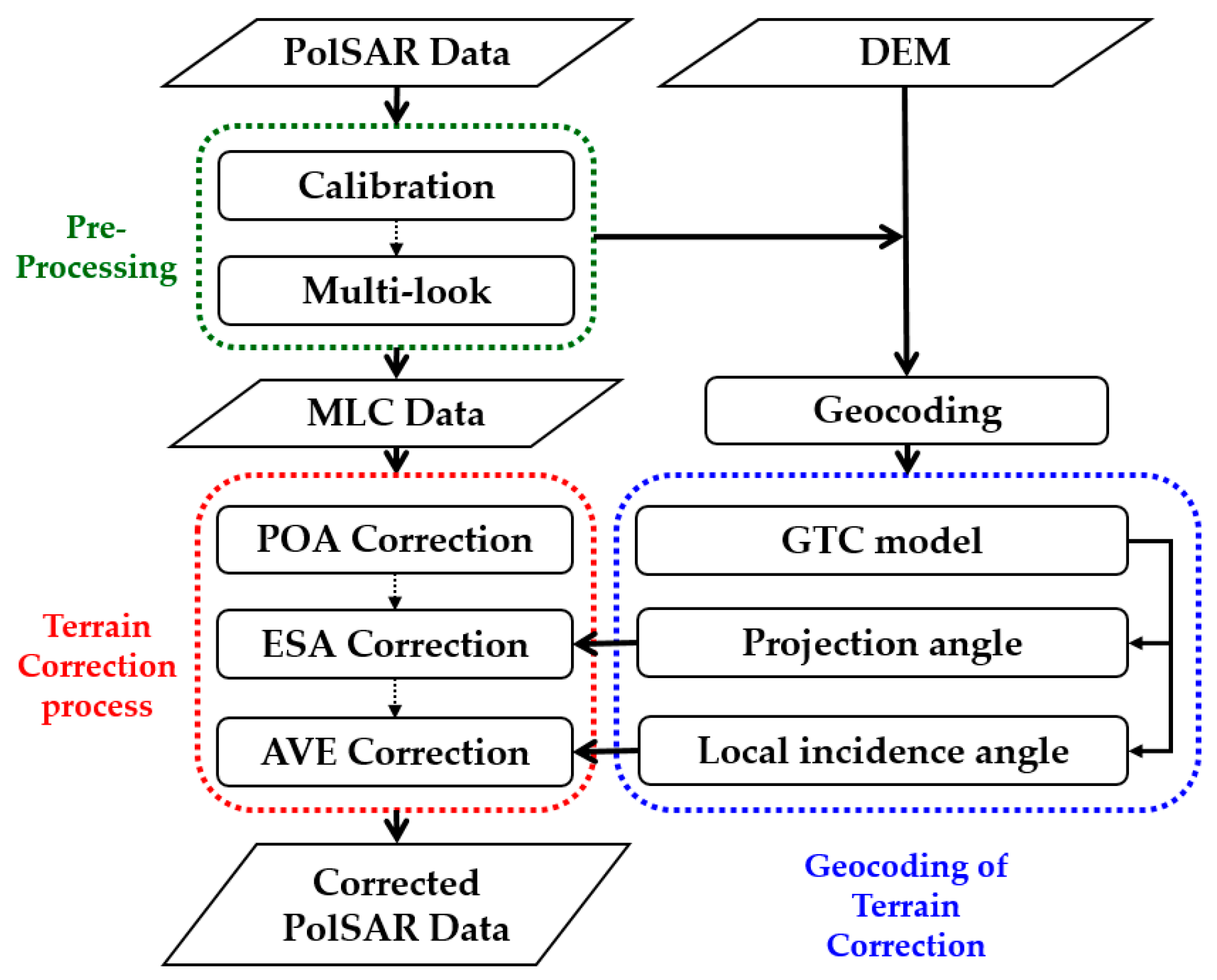
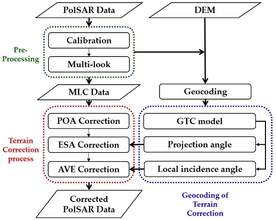
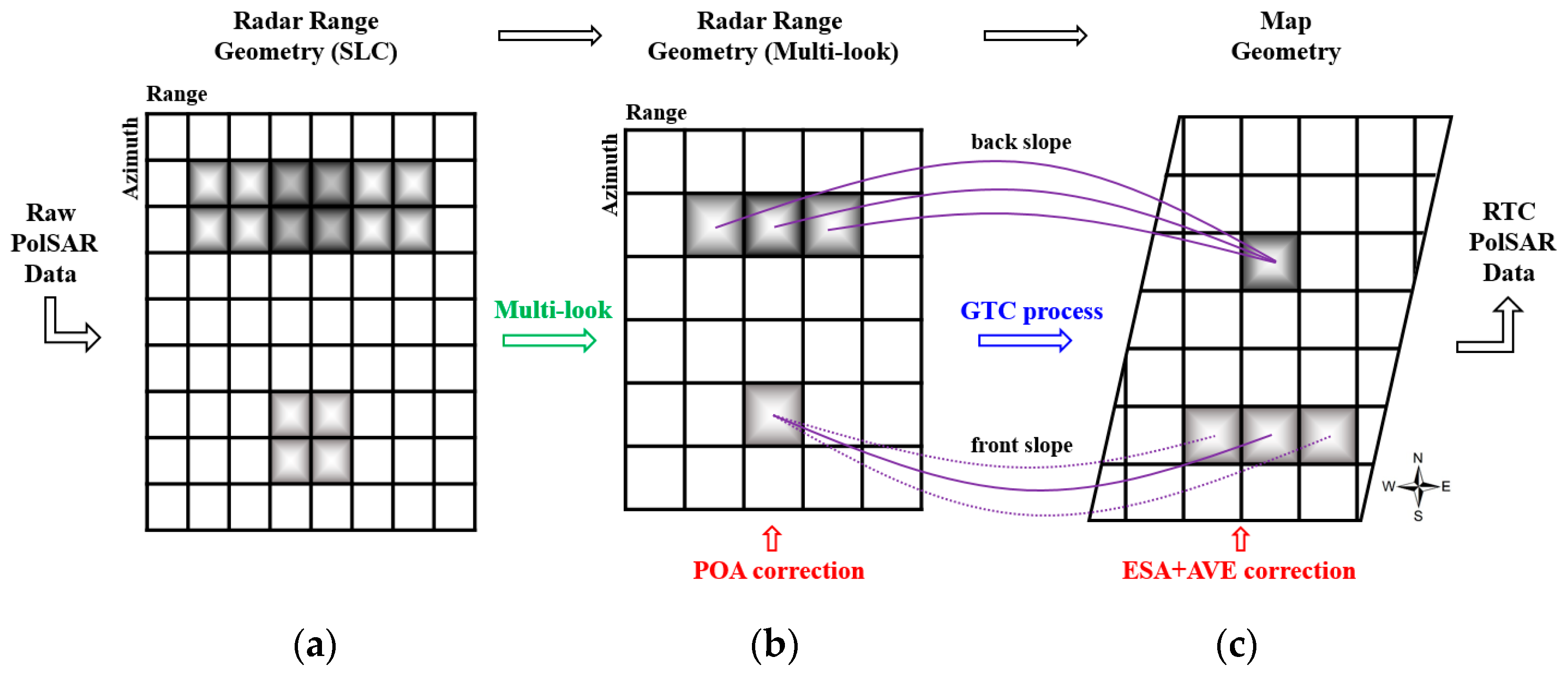
3.3.1. The Procedure of Terrain Correction

The PolSAR image terrain correction includes three steps: POA, ESA, and AVE corrections. Among these, POA correction can be completed in the slant-range space of PolSAR images before the geocoding process. The two remaining correction processes can be completed in geographic space with the GTC model. For convenient comparison, we present all of our results in geographic coordinate space.
The integrated three-step terrain correction method can be described by:
CRTC = (VCVT)·cosψK.
First, the POA correction is completed based on the POA shift angle (Figure 12). The ESA correction is then performed based on the projection angle ψ (Figure 10). Finally, the AVE correction is implemented based on the correction coefficient matrix K.
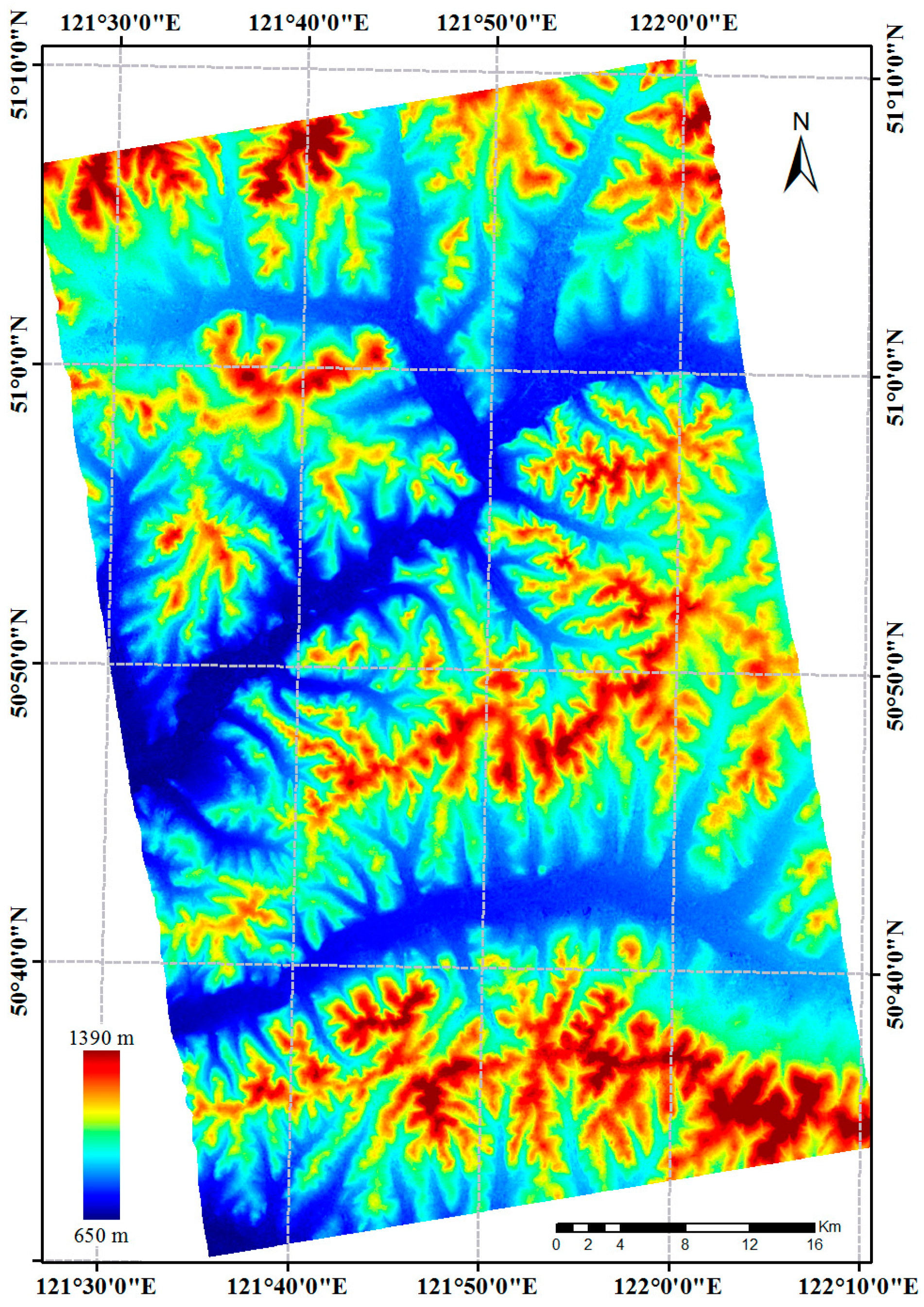
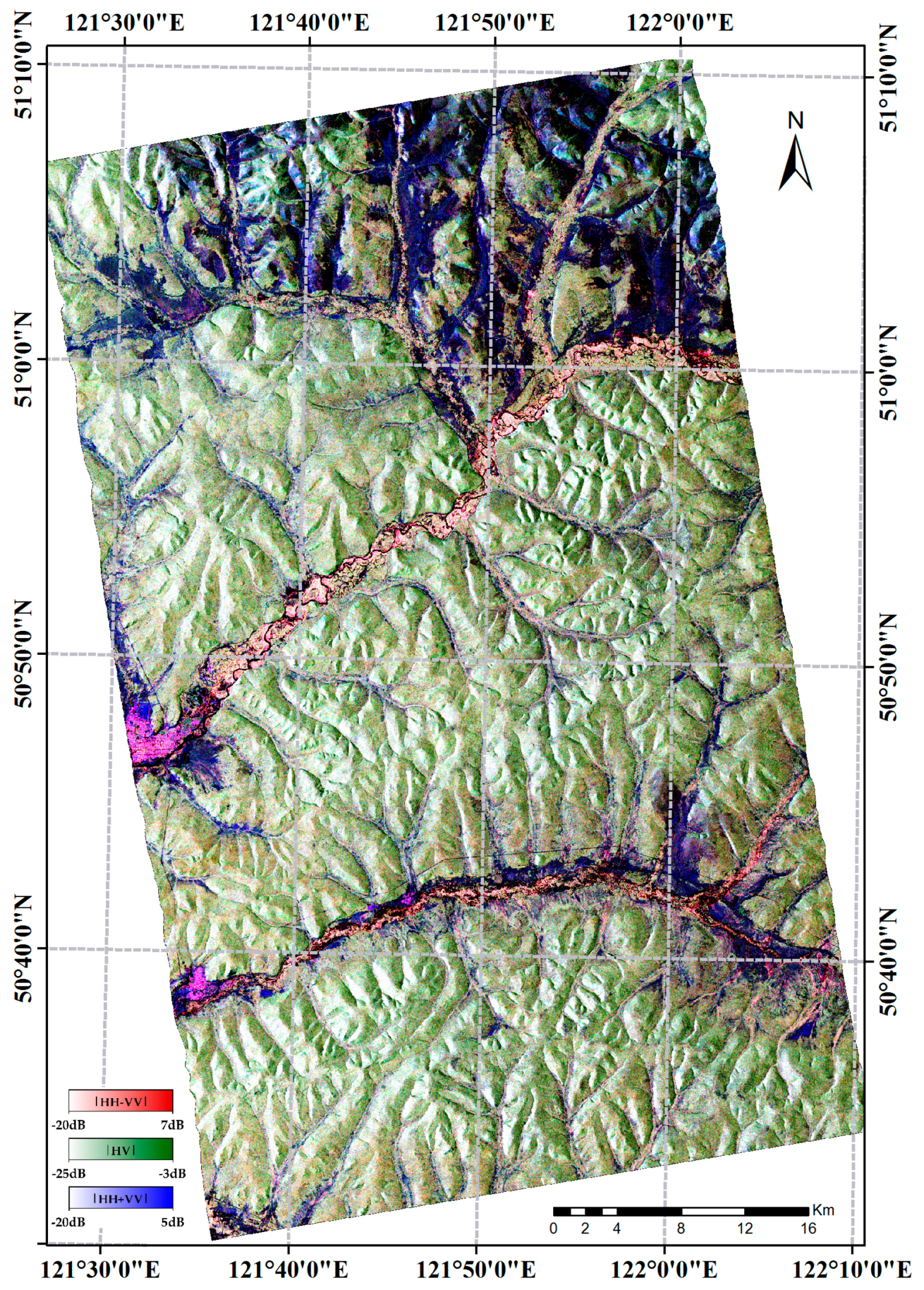
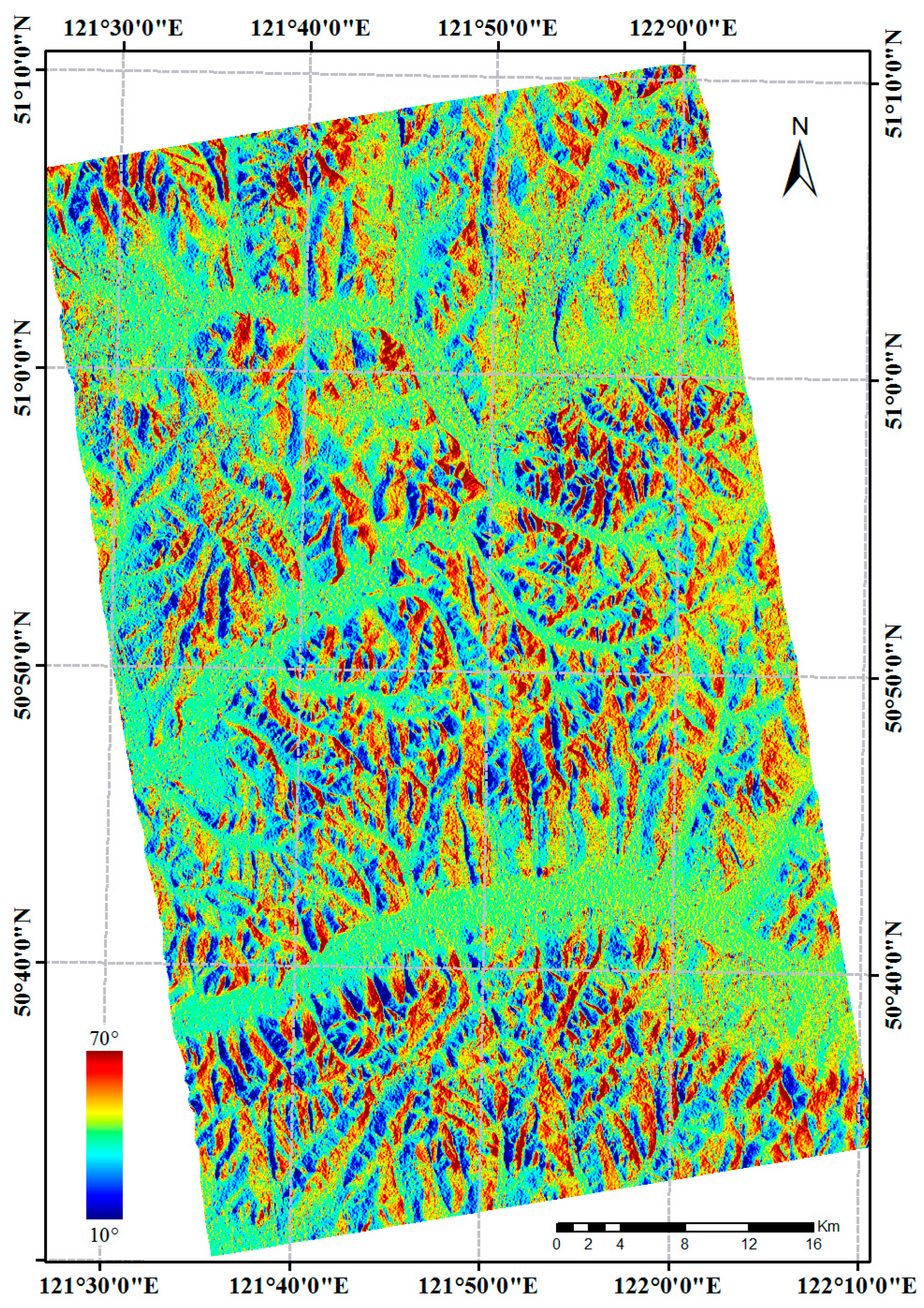
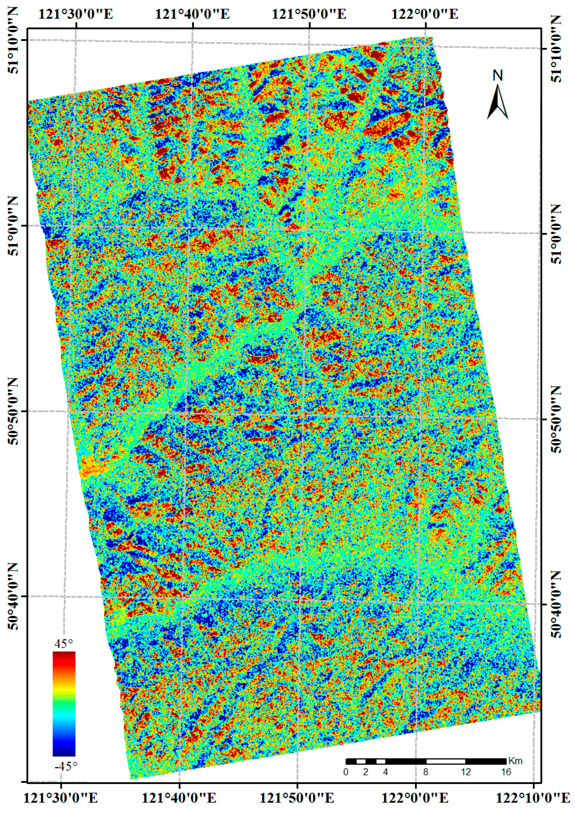
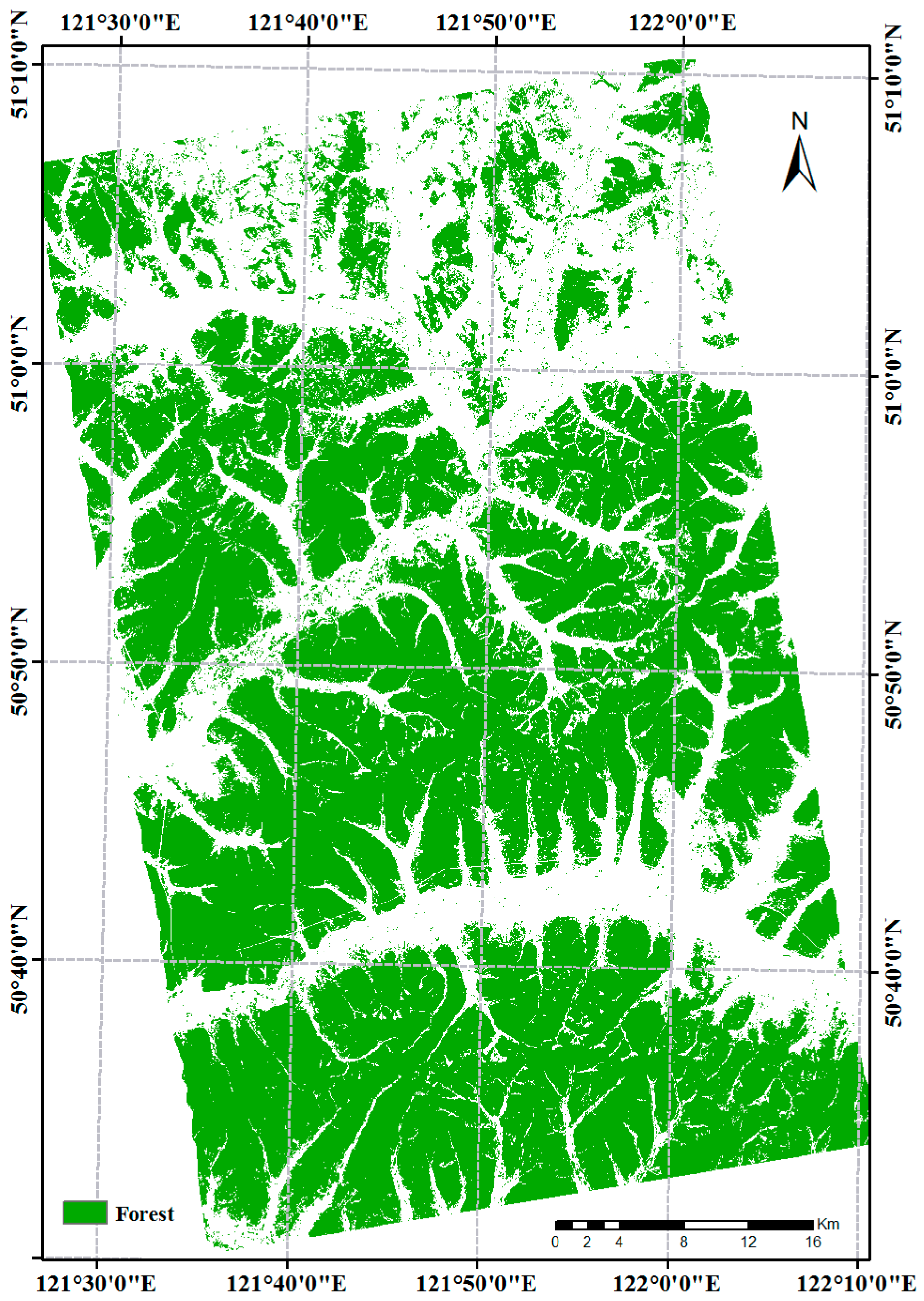
AVE correction requires the ability to distinguish land cover types. At our test site, forest is the dominant land cover, and it grows on areas with complex topography (Figure 9), whereas non-forest areas are mainly distributed on the flat terrain (Figure 8). Based on the PolSAR data following POA and ESA corrections, the forest cover map (Figure 13) may easily be obtained by unsupervised classification using polarimetric decomposition and the complex Wishart classifier [
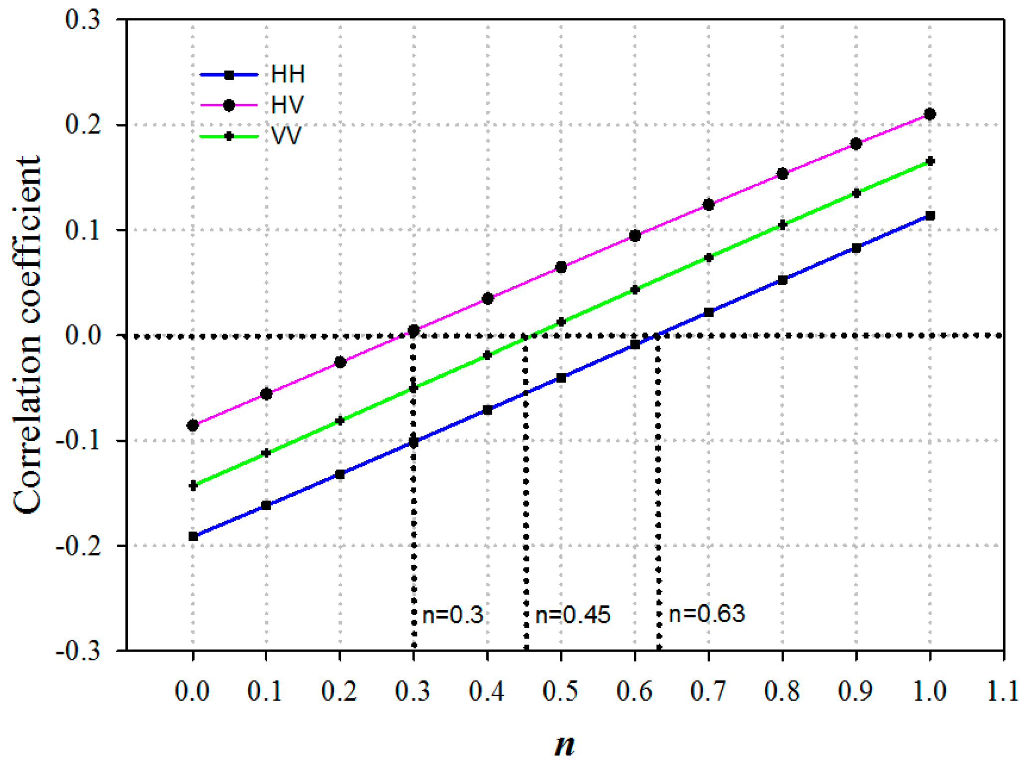
20]. Using the forest cover map as a mask file, we may then calculate the correlation coefficients between the AVE corrected backscattering values and the local incidence angle for various values of n (Equation (10)). The results are shown in Figure 14.
Figure 14 shows the correlation coefficients for the AVE corrected backscattering values for different polarisations and the local incidence angle as a function of n. The correlation coefficients for different polarisations corresponding to the same value of n are different, such that we should use different n values for different polarisations during the AVE correction. In general, the effective range of n is 0–1 [13]. Using an iterative method at the effective range, we may easily determine the optimum value of n when the correlation coefficient (Equation (12)) converges to a minimum value. In this study, the optimum values of n for different polarisations were nhh = 0.30, nhv = 0.45, and nvv = 0.63. With these values of n, we may obtain the final correction matrix K as:
K = [ k ( 0.30 ) k ( 0 . 75 ) k ( 0 . 93 ) k ( 0 . 75 ) k ( 0.45 ) k ( 1 . 08 ) k ( 0 . 93 ) k ( 1 . 08 ) k ( 0.63 ) ] .
If n equals 1 for different polarisations, the result of the AVE correction is a standard backscatter coefficient γ0 [10], which is frequently used in research on forest areas [4]. The γ0 is essentially a special case of the AVE correction model. Therefore, it may be not suitable in all situations. An analysis of n based on Figure 14 shows that a uniform and fixed value of n is not an ideal choice for PolSAR data.

3.3.2. Analysis of Terrain Correction Results

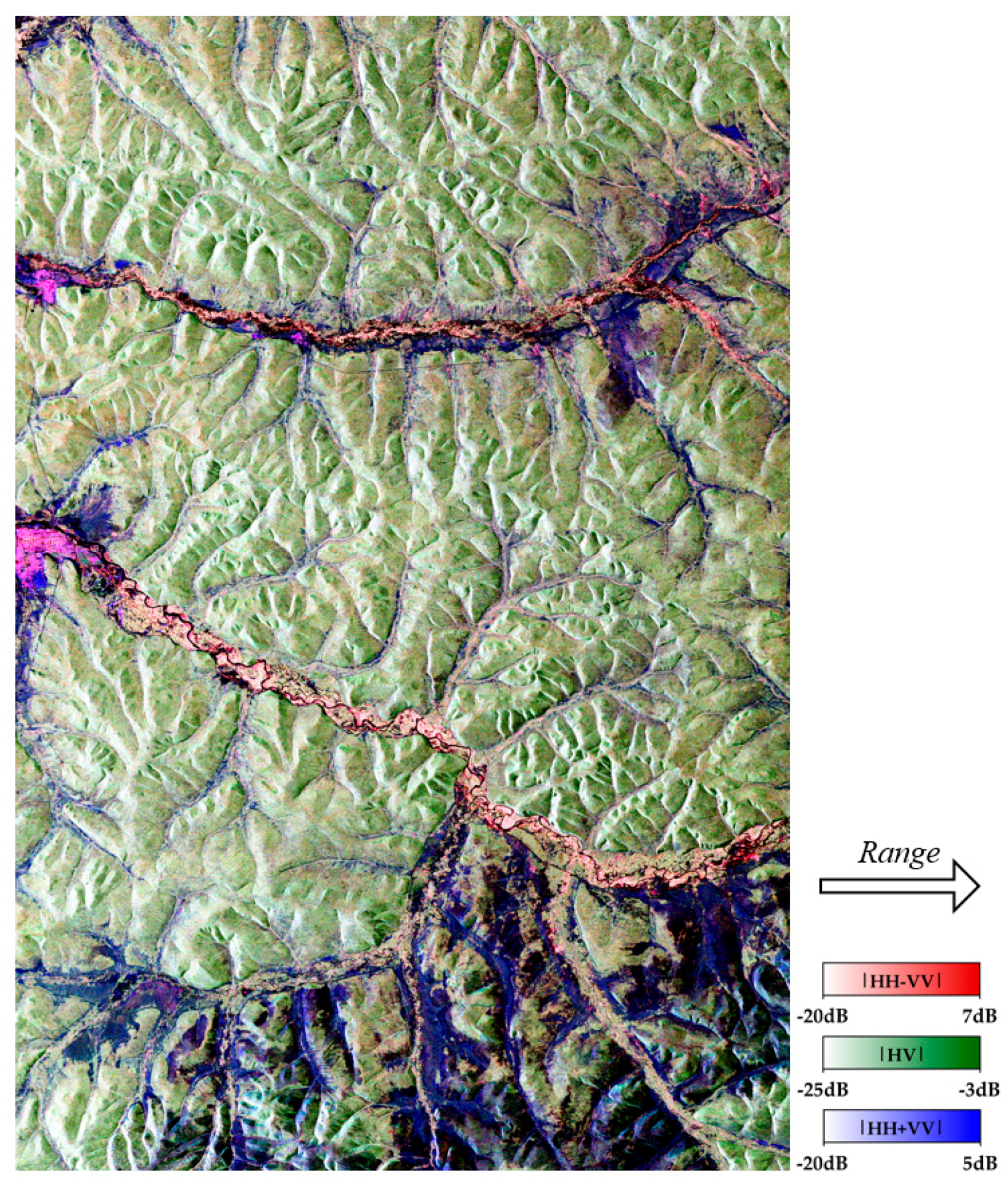
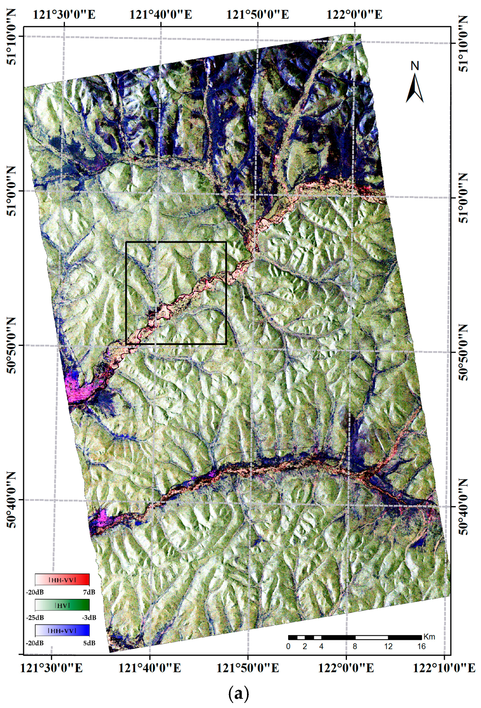
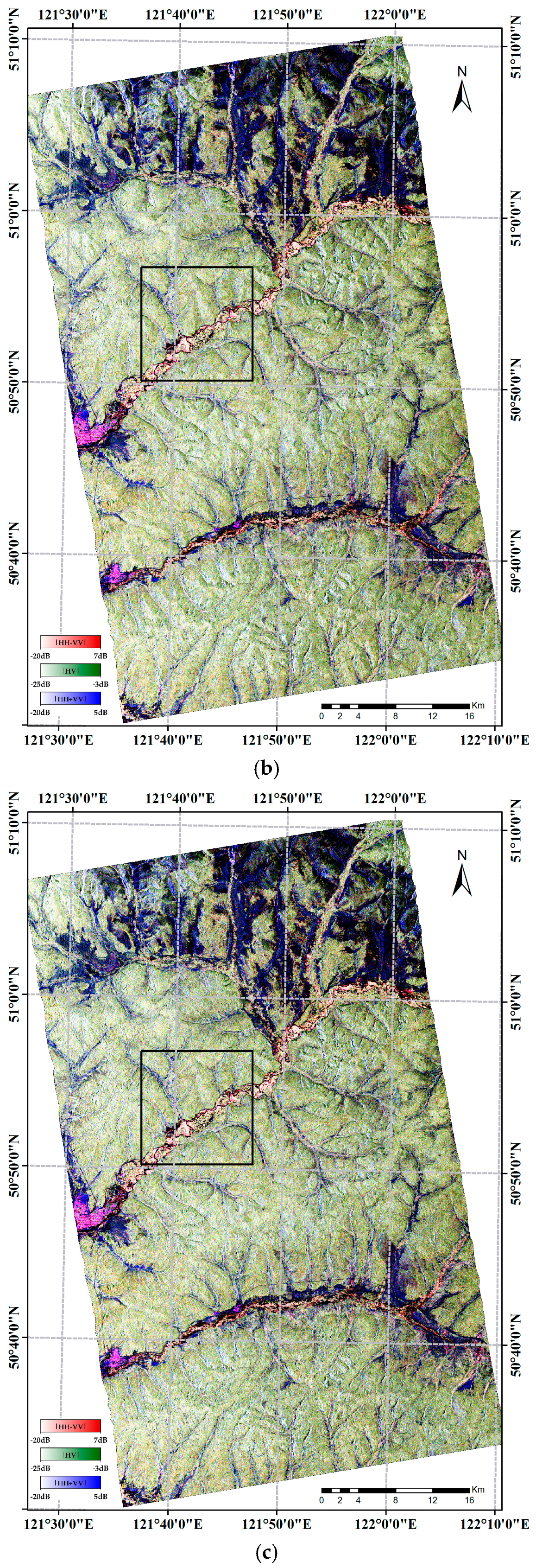
Figure 15a presents the Pauli RGB image of PolSAR data after POA correction. Compared to the uncorrected case (Figure 9), there appears to be no significant difference. This is because visual terrain effects on PolSAR image results are mainly due to the difference between front and back slopes in the range direction. In contrast, the impact of azimuth terrain is relatively weak in the case of an entire scene PolSAR image. Thus, there are no obvious visual changes after POA correction. Figure 15b shows further results after ESA correction. The radiometric distortions due to terrain relief were strongly reduced compared to the PolSAR images shown in Figure 9 and Figure 15a. However, there are still subtle topographic effects on local details of the PolSAR image. The final result after AVE correction is shown in Figure 15c. Topographic effects have effectively been removed from Figure 15b, and there is no obvious visual difference between the pixels on the front and back slopes.
Because the range of the PolSAR image is large, Figure 15 appears small. Details in the PolSAR images are not easy to observe. Therefore, we display an enlarged area in Figure 15 (black polygon) for more detailed demonstration (Figure 16). Enlarged images of GTC PolSAR, POA shift angle, and local incidence angle are shown in the area. In the enlarged images, greater detail of different correction steps may be seen, particularly when compared to the enlarged images of POA shift angle and local incidence angle. For example, in the regions where the POA shift angle is larger (Figure 16e, red), the PolSAR image of GTC (Figure 16a) is greener than the PolSAR image for the POA correction (Figure 16b). This means that cross-polarisation was overestimated in these regions. Compared with the middle regions of Figure 16c,d,f, improvements made by the AVE correction may be seen more clearly.
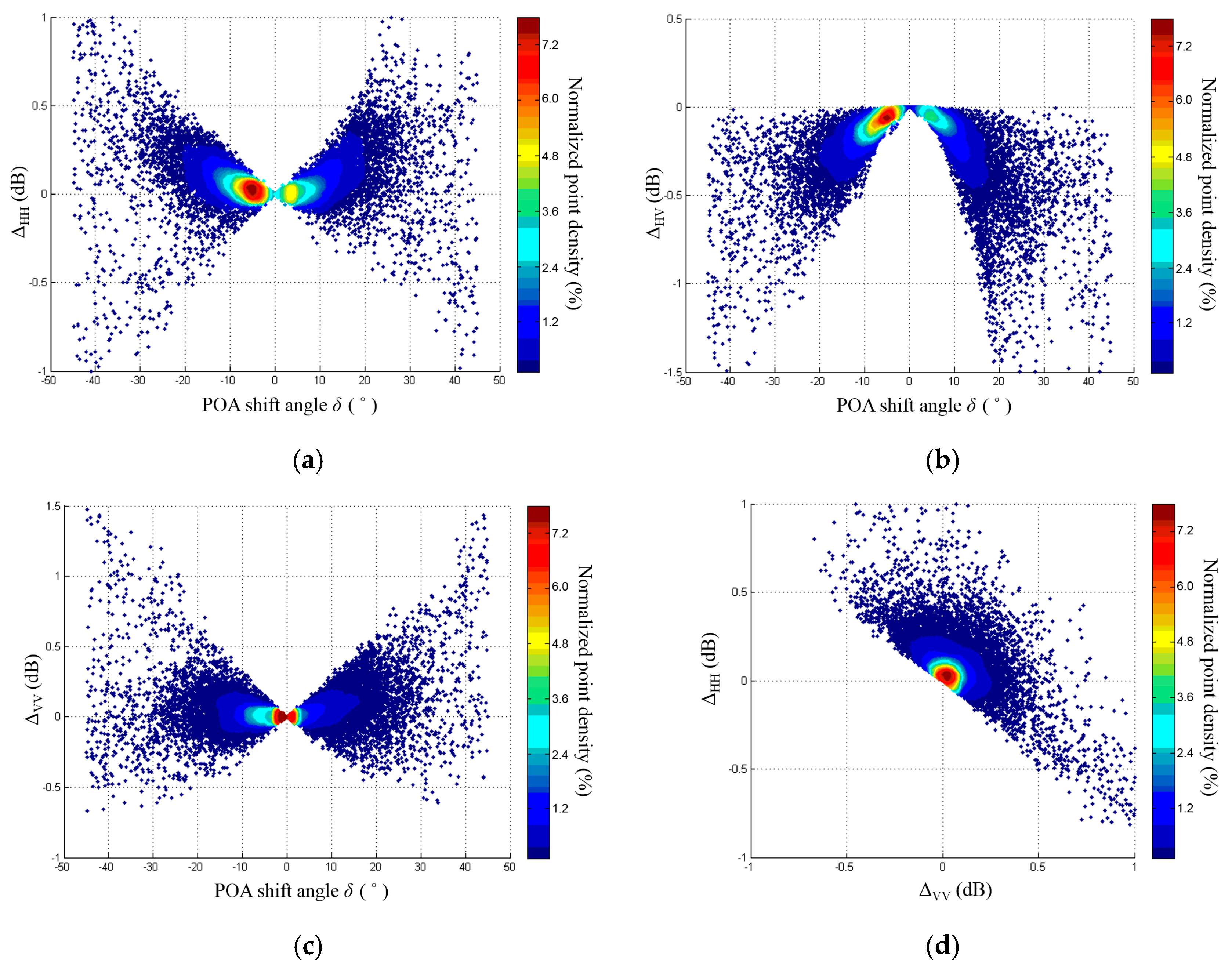
To evaluate the effectiveness of the three-step correction method, we conducted a deeper analysis. For the POA correction, the relationships between the POA shift angle and the differences between corrected and uncorrected PolSAR data were analysed.
As shown in Figure 17, ΔHH, ΔHV, and ΔVV were the differences between the corrected and uncorrected backscattering coefficients for different polarisations (corrected − uncorrected pixel values). With increasing POA shift angle, the numerical ranges of ΔHH, ΔHV, and ΔVV increased. The values of ΔHH and ΔVV may be positive or negative, and the proportion of positive values was relatively large; however, the value of ΔHV may only be less than zero. These patterns indicate that a POA shift will cause overestimation of the backscattering coefficient of HV polarisation. Because of the conservation of polarimetric span, HH and VV polarisation cannot be overestimated simultaneously; that is, ΔHH and ΔVV cannot be negative at the same time (
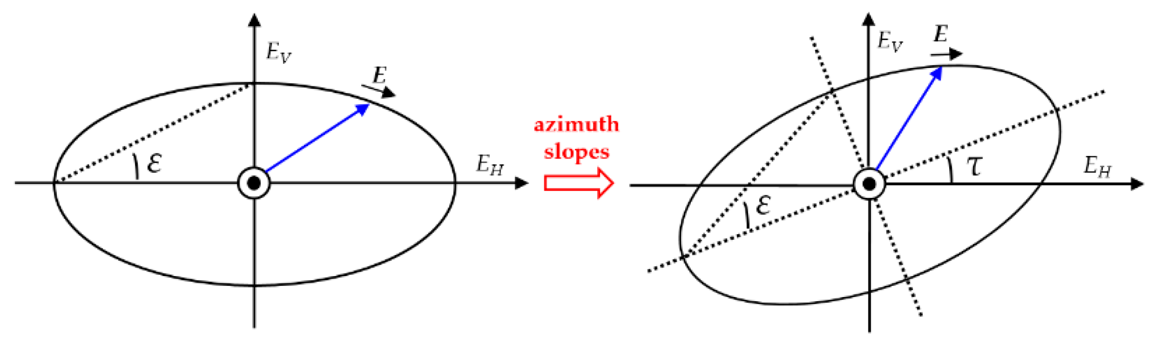
Figure 17d). Additionally, the POA shift exerted more influence on HV polarisation than HH and VV. For example, when the POA shifted by approximately 20°, the maximum biases of HH and VV polarisation were approximately 0.5 dB, while that of HV polarisation was greater than 1 dB. This also indicates that POA correction is an indispensable step for terrain correction of PolSAR data. These different behaviours can be explained by the physical basis of the POA shift. When polarimetric radar images a horizontal surface, the horizontal polarisation electric field of transmitted and received data is parallel to the surface. For a tilted surface, however, the horizontal electric field of transmitted data is no longer parallel to the horizontal surface. However, the horizontal electric field of received data is parallel to the tilted surface. Therefore, there is a shift in angle between the transmitted and received electromagnetic wave vectors. Consequently, the horizontal-transmitting and vertical-receiving (HV) components are increased and horizontal-transmitting and horizontal-receiving (HH) components are decreased, due to the tilted slope. In the case of a vertical polarisation wave, a similar phenomenon occurs. Therefore, the basic rule is that cross-polarisation (HV) will be overestimated and co-polarisation (HH + VV) will be underestimated due to the POA angle shift.
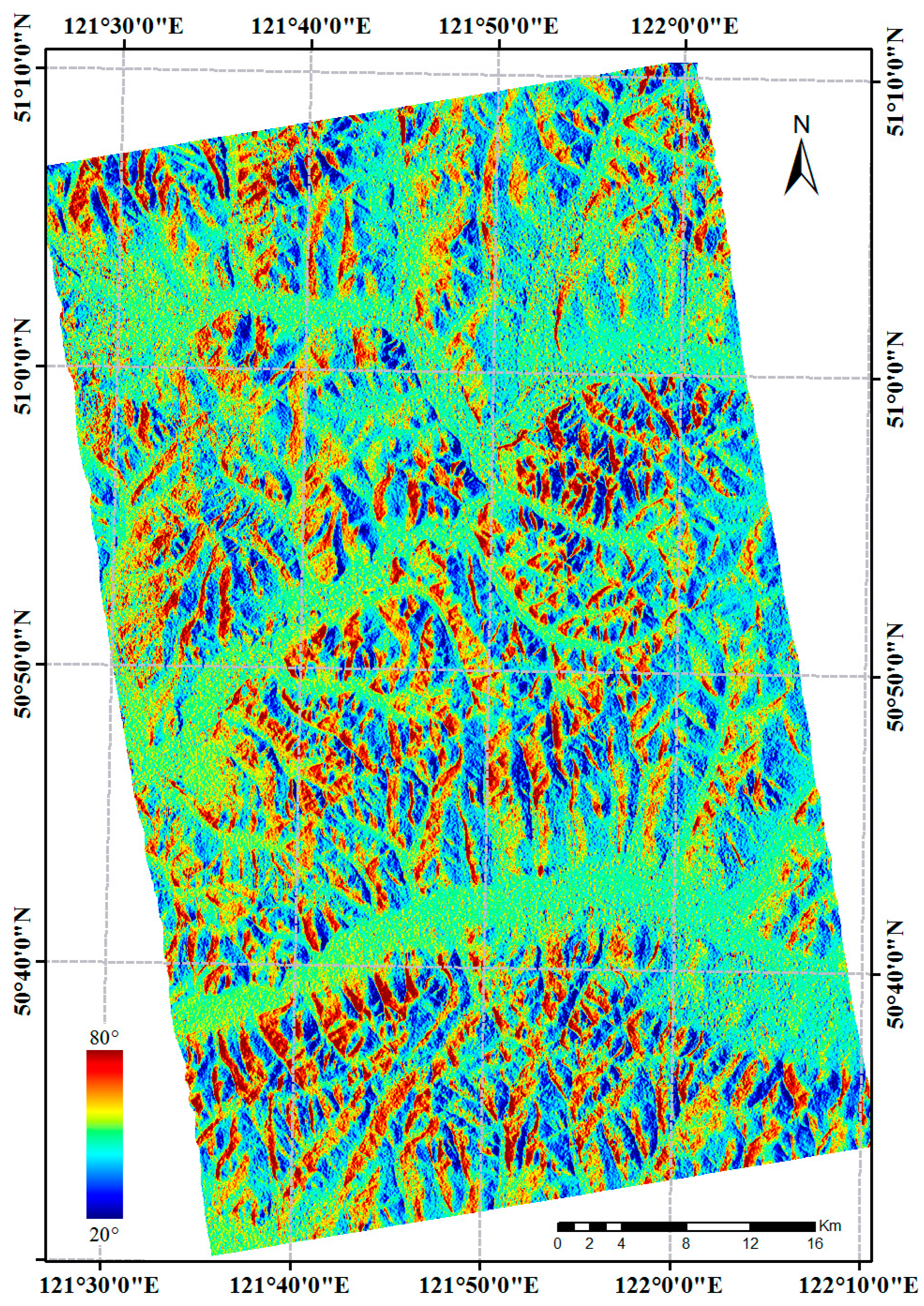
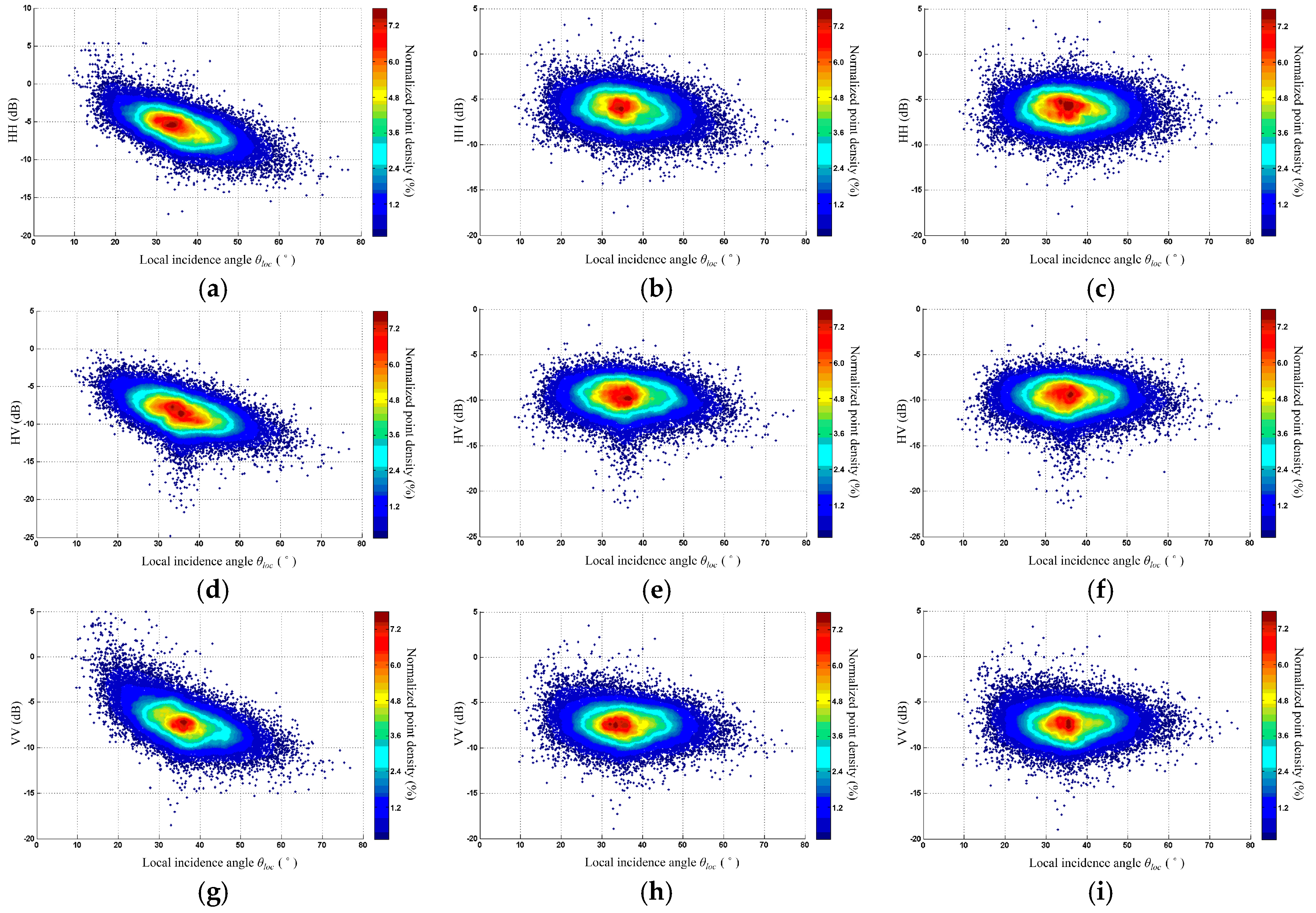
We then analysed the relationship between backscattering coefficients of different polarisations and the local incidence angles at different correction steps. Figure 18 presents the backscattering coefficients of different polarisations as a function of the local incidence angle (θloc). And we divided PolSAR data into three groups according to the 33.3th and 66.6th percentile of θloc, the statistical characteristics of each group were calculated and are displayed in Figure 19. For the PolSAR data without ESA correction (Figure 18a,d,g), clear linear relationships were found between the backscattering coefficient and θloc for each polarisation channel. We observe higher backscattering values for the small θloc of front slopes, and lower values for the large θloc of back slopes. The difference of backscattering value between large θloc group and small θloc group is about 3 dB (Figure 19). Following ESA correction (Figure 18b,e,h), this phenomenon was effectively relieved. And the difference of backscattering value between large θloc group and small θloc group is reduced to about 0.5 dB (Figure 19). However, as θloc increased, backscattering values continued to decrease. Complex terrain effects on the corrected PolSAR data clearly remain (Figure 15b and Figure 16c). However, as shown in Figure 18c,f,i, the residual terrain effect was further removed by AVE correction. And the difference of backscattering value between large θloc group and small θloc group is reduced to about 0.1 dB (Figure 19). These behaviours are due to the scattering mechanism of the actual forest; it cannot be pure surface scattering or ideal volume scattering. In the case of an ideal surface scattering target, ESA correction was sufficient. For an ideal volume scattering target, γ0 was more suitable, in that it remained approximately constant for all incidence angles [21]. Therefore, this may be the reason why ESA correction is insufficient and AVE correction is required.
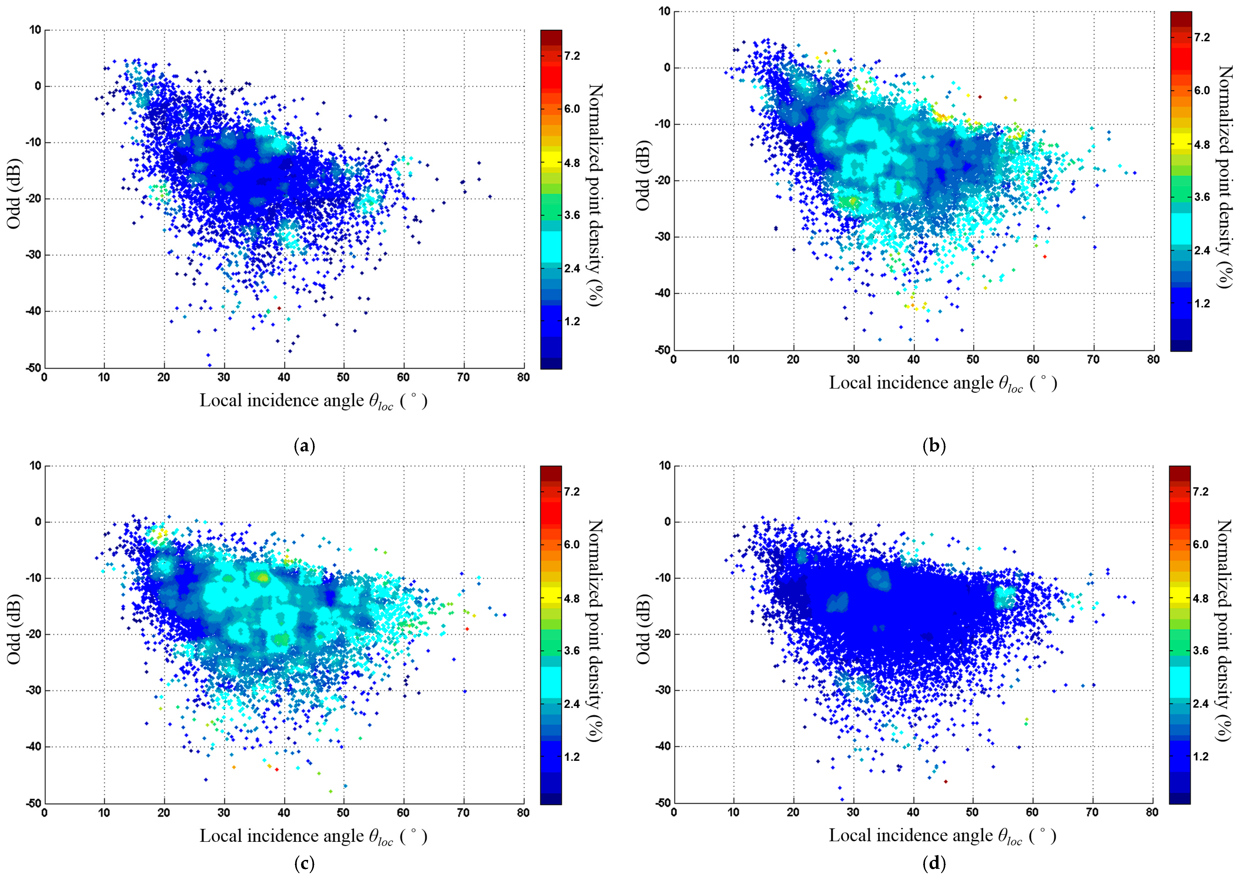
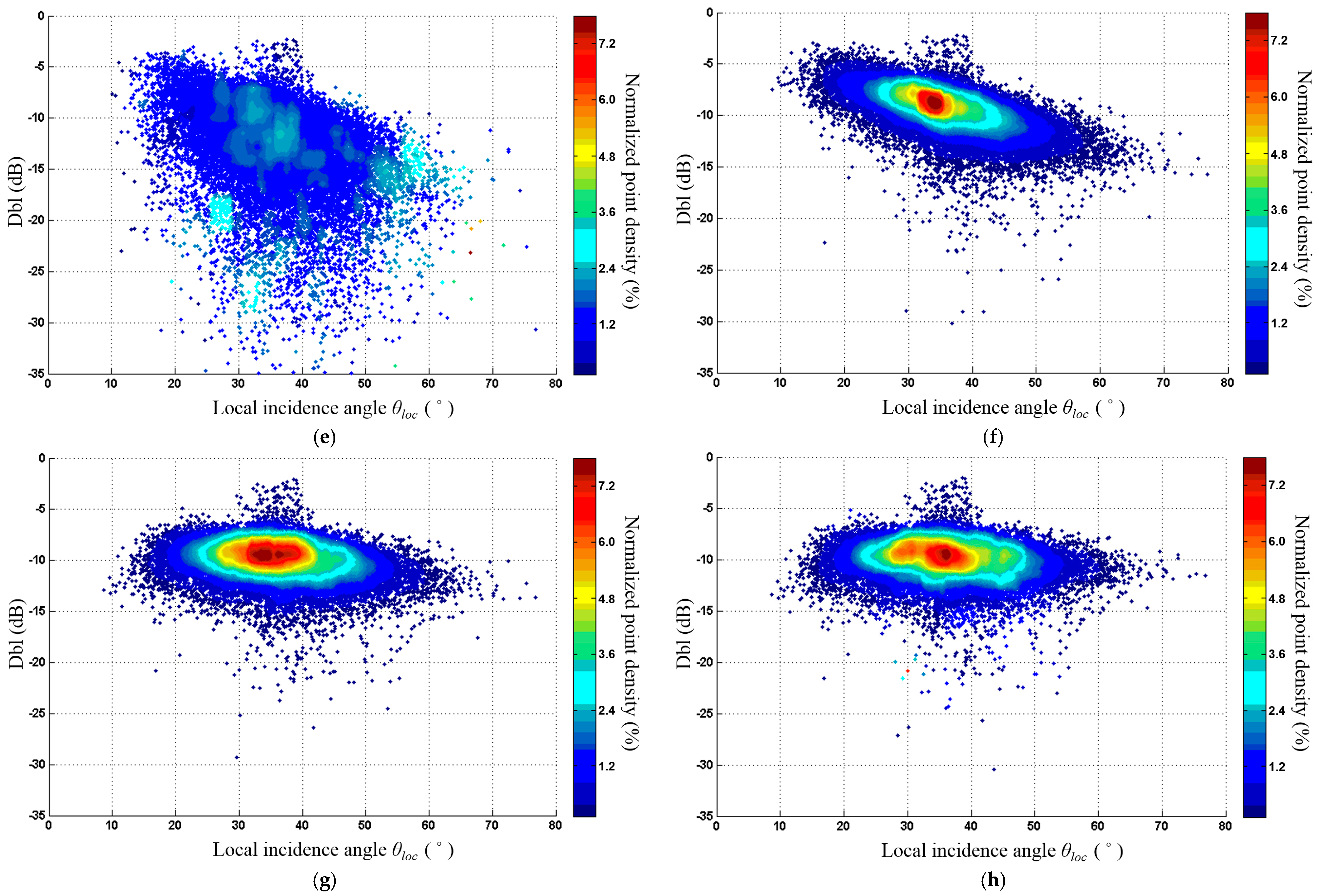
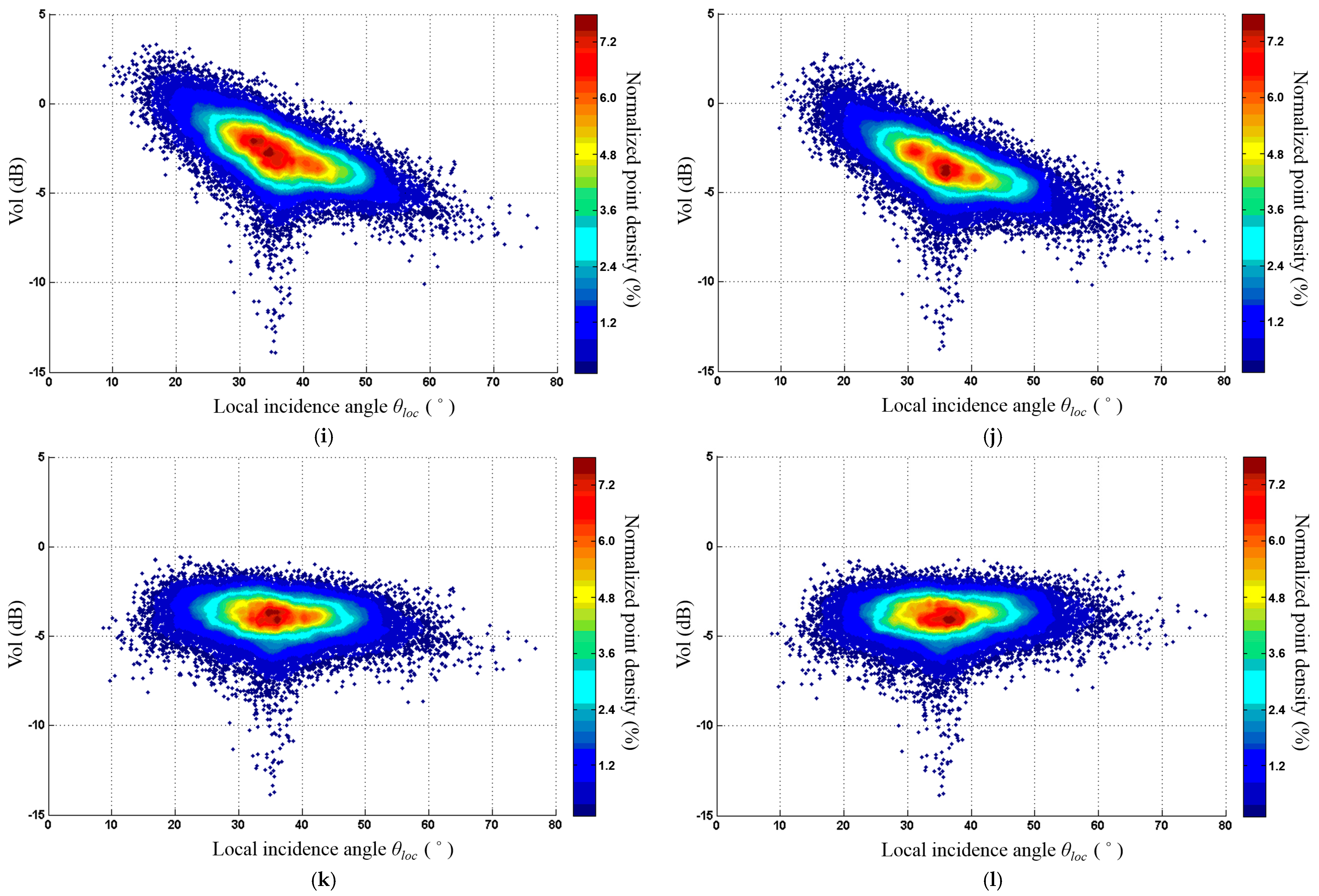
Using the Yamaguchi four-component decomposition as an example [22], we also analysed the relationship between polarimetric decomposition parameters and the local incidence angle at the different correction steps (Figure 20). These four polarisation parameters can be obtained from PolSAR matrix data at different correction steps by Yamaguchi four-component decomposition, which includes surface scattering power (Odd), double-bounce scattering power (Dbl), volume scattering power (Vol) and helix scattering power (Hlx). As shown in Figure 20a,e,i,m, the decomposition parameters derived from GTC PolSAR data and also as a function of the local incidence angle exhibit linear behaviour, with higher decomposition parameter values for low θloc, and lower values for the high θloc. ESA correction also plays a major role in determining all decomposition parameters. This is because a larger ESA value corresponds to larger decomposition components. Comparing the scatter plots for the different correction steps, the behaviour at different correction steps is similar to that shown in Figure 18. For the Odd and Hlx components, the terrain effect was relieved only at the ESA correction step. In the case of the Vol component, the terrain effect was relieved mostly at the ESA correction step, whereas AVE correction can further remove the residual terrain effect. However, for the Dbl component, all three correction steps were useful. The POA correction significantly reduced the dispersion of the points (Figure 20f), and ESA and AVE corrections further removed terrain effects (Figure 20g,h). This result may be due to the correction of not only the principal diagonal elements but also non-diagonal elements of the polarisation covariance matrix. Overall, the RTC results indicate that the best correction results were due to the Dbl and Vol components, which were the dominant scattering mechanism for the forest. ESA correction was still the most important correction step, but only ESA correction fails to remove the terrain effects completely.

3.3.3. Effectiveness of the Three-Step RTC for Forest AGB Estimation

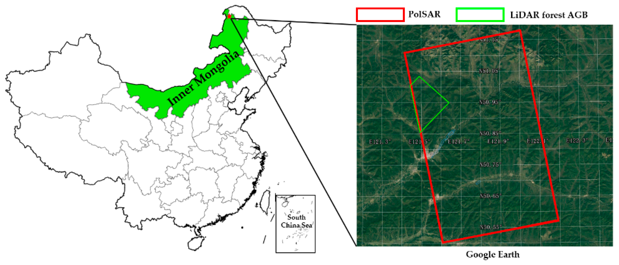
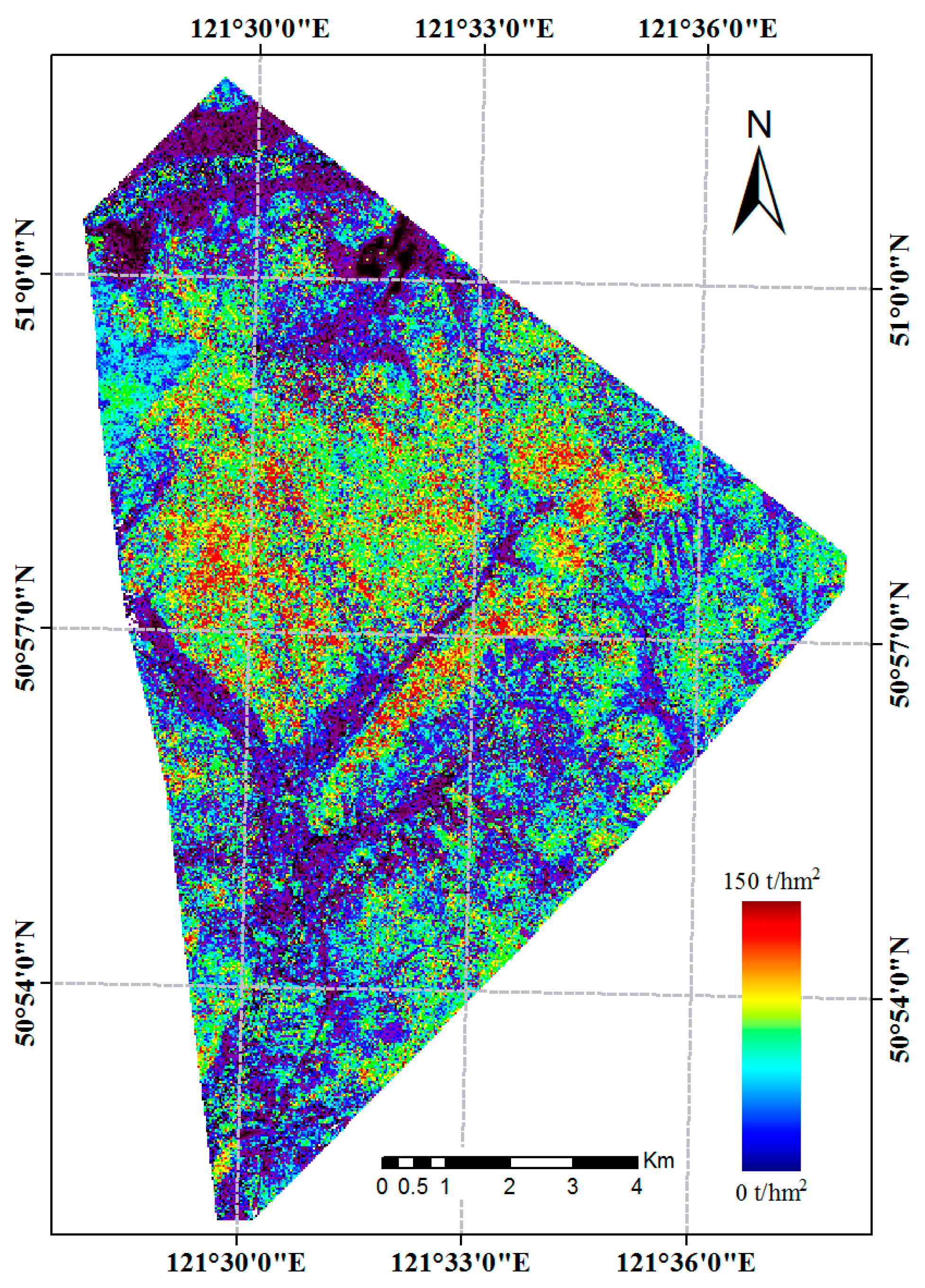
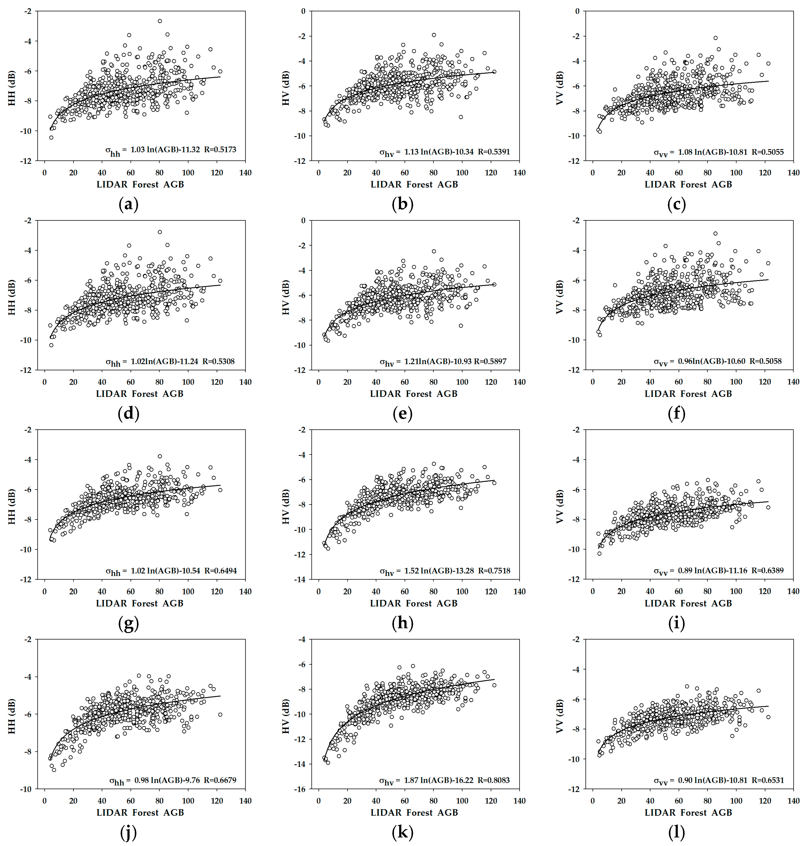
One of the key applications of RTC in forest areas is to reduce biomass estimation error caused by uneven topography. For further verification of the effectiveness of the three-step RTC method for forest AGB estimation, we analysed the relationship between the LiDAR-derived forest AGB data and the backscattering coefficients of the uncorrected (GTC) and corrected (POA, POA + ESA, POA + ESA + AVE) PolSAR data at the test site (Figure 5, green rectangle; Figure 7), as shown in Figure 21. Black lines indicate the regression curve of a logarithmic equation. The correlation coefficient (R) of regression model was calculated and displayed in each plot. The method of statistical regression is least squares can refer to [23]. There were 518 points in each plot, which were extracted from LiDAR-derived AGB data and PolSAR data for different correction steps. To ensure the reliability of the results, non-forest points were masked and the points at the forest edge were also excluded. The spatial interval between two points is 90 m, and the value for each point was a mean value of the surrounding pixels. Thus, the influence of geographical coordinate error between LiDAR data and PolSAR data was reduced.
Figure 21a–c shows the scatter plots of LiDAR-derived forest AGB and backscattering coefficients before three-step RTC processing, and Figure 21d–l shows the same result after processing at each correction step. This shows that three-step RTC can significantly reduce the dispersion of the points. All of the correlations between the backscattering coefficients of each of the three polarisations and the forest AGB were improved; the lowest R value in the POA + ESA + AVE correction step (Figure 21j–l, VV polarisation) was larger than the highest R value in the uncorrected case (Figure 21a–c, HV polarisation). The backscattering coefficients for HV polarisation after RTC processing (Figure 21k) had the best correlation with forest AGB, whose R value was 0.8083, while the corresponding R value for HV polarisation before RTC processing was only 0.5391. The contributions of POA, ESA and AVE to correlation coefficient were 0.05, 0.16 and 0.06, respectively. In the case of co-polarisation, similar phenomena were observed.
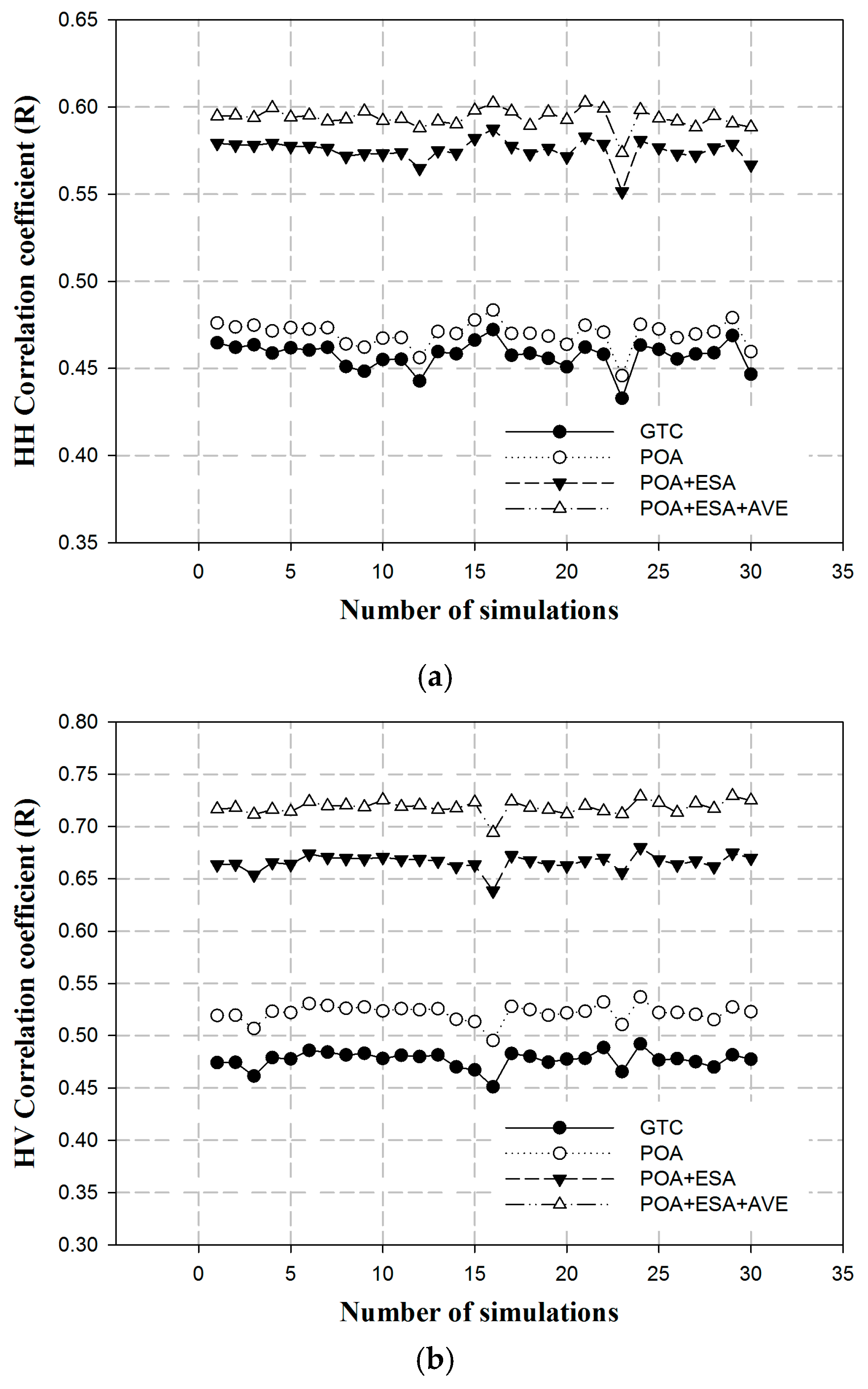
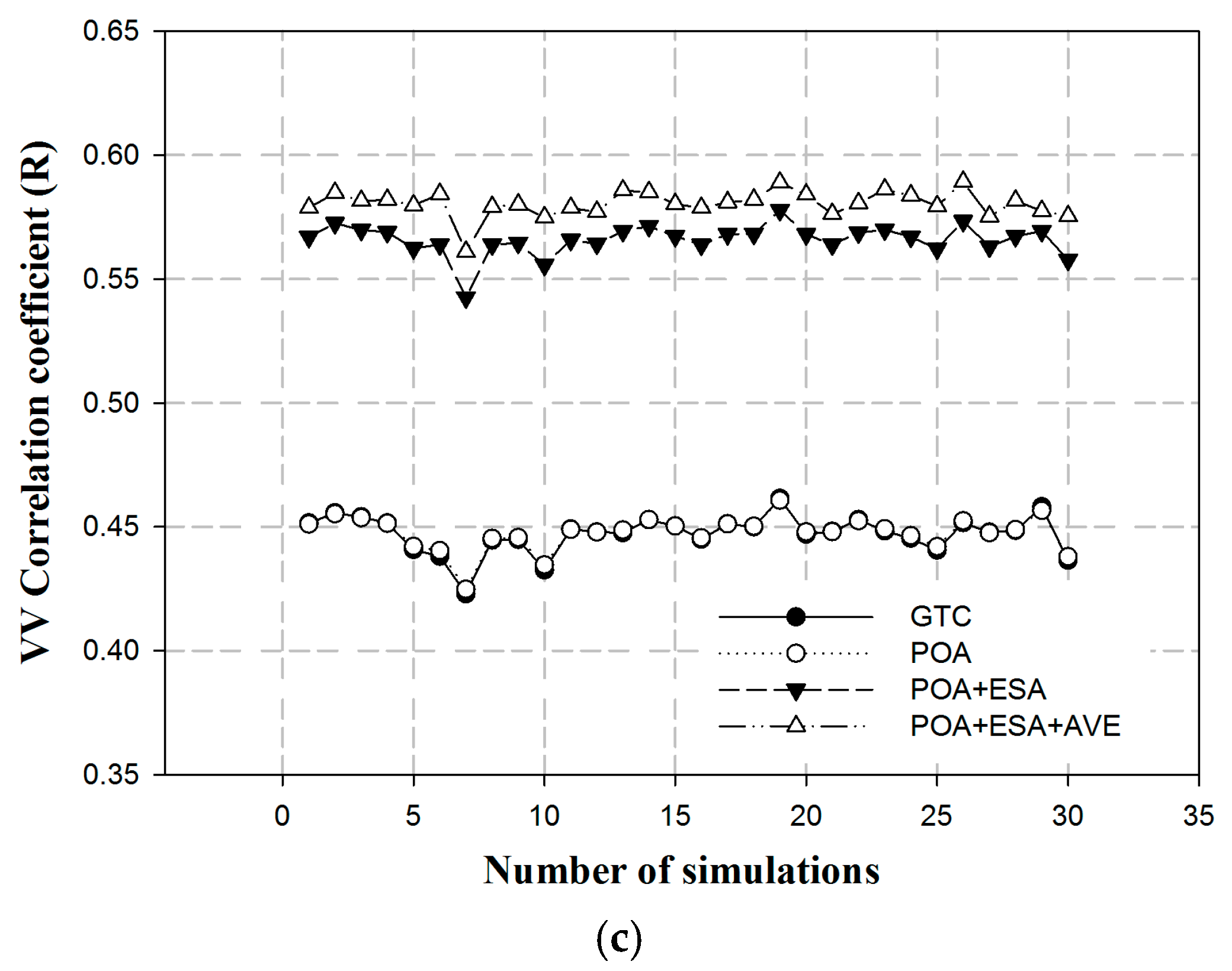
To evaluate the robustness of the regression results, we conducted an uncertainties analysis of LiDAR forest AGB and backscattering coefficients of different correction steps. For the former, the uncertainty is mainly due to the estimation error of forest AGB. For the latter, the uncertainty is mainly due to the accuracy of the DEM data. First of all, an additional error term of Gaussian distribution (Mean: 0; Standard deviation: 23.1 t/hm2) was added in the LiDAR forest AGB. The standard deviation of error term is equal to the RMSE of LiDAR forest AGB. Based on this error term, simulated forest AGB data can be generated and used for regression. We calculated the correlation coefficients for each regression, as shown in Figure 22. Overall, the correlation coefficient of different polarisation and different correction step decreased due to the additional error terms. However, the proportion of the contribution of different correction steps to correlation coefficient is consistent with Figure 21. In HV polarisation, for example, the mean contributions of POA, ESA and AVE were 0.04, 0.15 and 0.05, respectively.
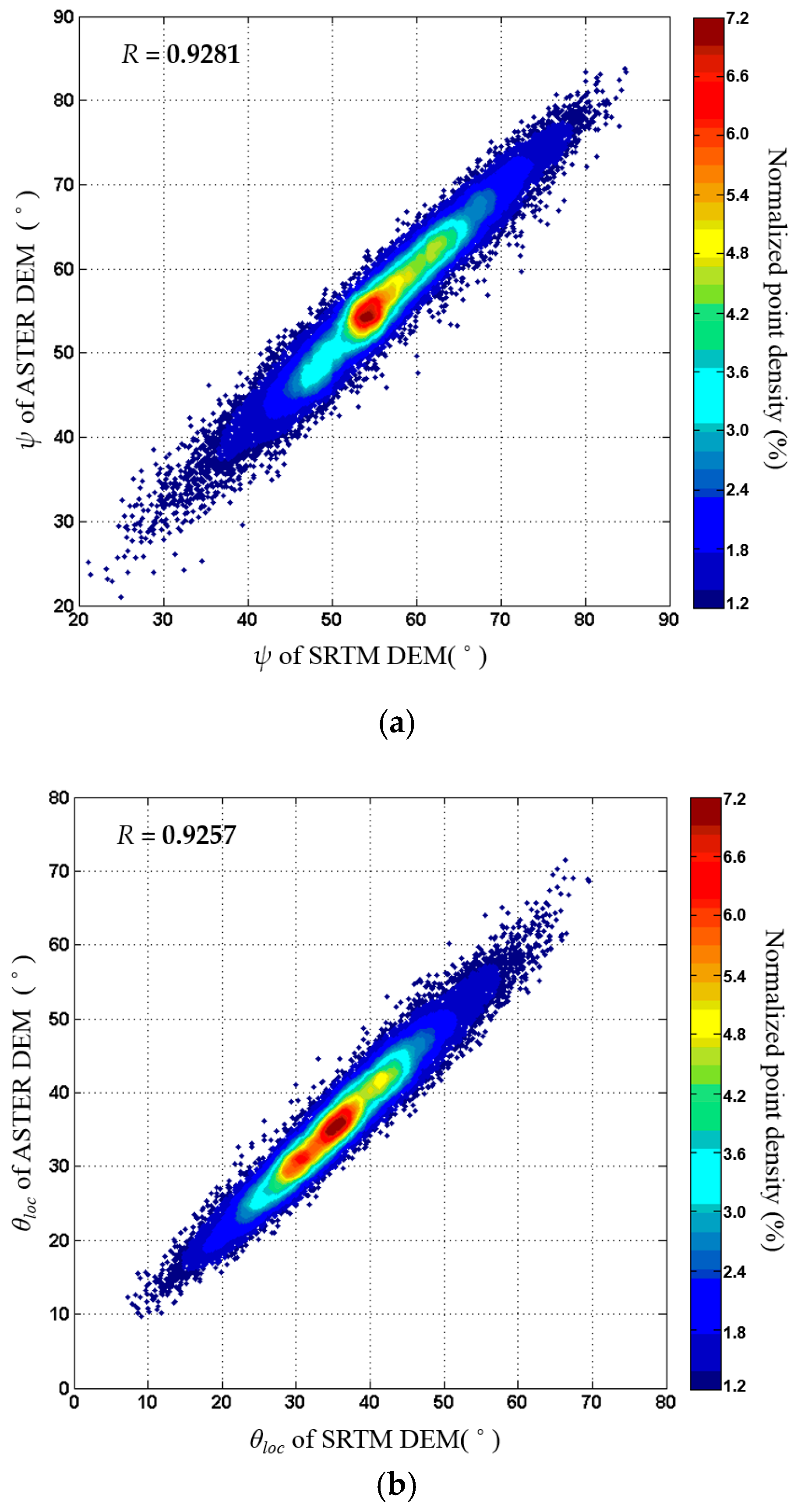
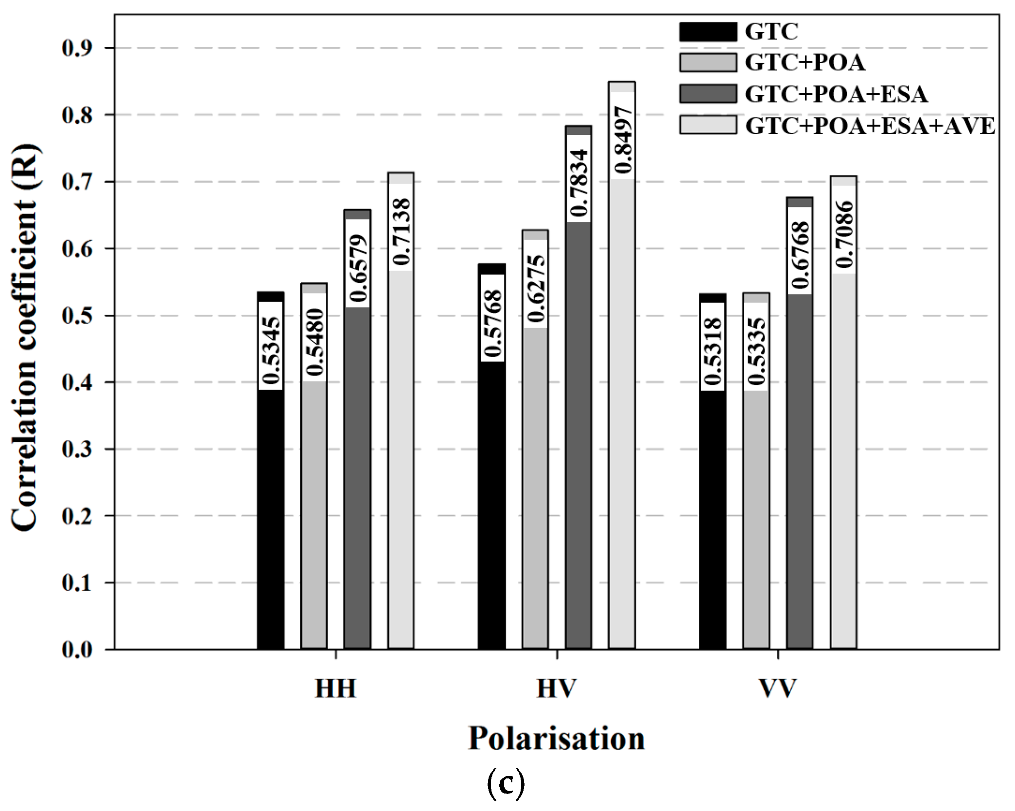
Secondly, it is the uncertainty caused by DEM. In this respect, we re-verified the results using SRTM DEM (30m). Figure 23 shows the validation results. In repeated experiments, the geocoding accuracy of azimuth and range directions were 0.17 and 0.22 pixels in the GTC process. This is slightly higher than the accuracy based on ASTER DEM. And the optimum values of n for different polarisations were nhh = 0.31, nhv = 0.49, and nvv = 0.61. This is basically consistent with the ASTER DEM-based parameters. Figure 23a shows the correlation between ψ of ASTER DEM and ψ of SRTM DEM, whose R value was 0.9281. And Figure 23b shows the correlation between θloc of ASTER DEM and θloc of SRTM DEM, whose R value was 0.9257. This shows that similar imaging geometric angles were achieved by SRTM DEM compared with ASTER DEM. Figure 23c shows the correlation coefficient between backscattering coefficients of different correction steps and LiDAR forest AGB. We can see that similar results were obtained based on SRTM DEM compared with ASTER DEM. In HV polarisation, for example, the R value of GTC, POA, ESA and AVE were 0.5768, 0.6275, 0.7834 and 0.8497, respectively. The contributions of POA, ESA and AVE to correlation coefficient were 0.05, 0.16 and 0.07, respectively. Overall, the R value of SRTM DEM were slightly higher than that of ASTER DEM. The reason may be that higher geocoding accuracy and more reliable imaging geometric angles can be obtained by SRTM DEM compared with ASTER DEM. However, this requires further and more detailed researches to confirm.
Thus, we conclude that the three-step RTC method improves the power of PolSAR data to estimate forest AGB in uneven topography conditions. There is no doubt that ESA correction is the most important correction for improving biomass estimation, although POA and AVE corrections are also important. Additionally, the method developed in this study is fully suitable for PolSAR data in a matrix format, for example, covariance or coherency matrices. We can also extract the most sensitive polarisation parameters from the matrix data after RTC processing to construct a forest AGB inversion model, which will further improve model performance.

4. Discussion

The RTC method proposed in this study consists of three steps, in which POA and ESA corrections are based on a physical interpretation of polarisation theory and the SAR imaging geometry model, whereas AVE correction is based on a semi-empirical model. Therefore, in general, this method is a semi-empirical RTC method. Our results have verified the effectiveness of the method.

4.1. Limitations of DEMs for Geocoding and ESA Correction

The first step of terrain correction is to geocode the SAR data with DEM data of sufficient resolution. For most users, free, globally shared DEM data, for example, ASTER DEM, SRTM DEM and ALOS 3D DSM, are the only data sources that may be employed. However, these DEM data are not actually digital elevation models, but digital surface models. Therefore, the RTC process proceeds under the assumption that the top of the forest canopy follows the underlying topography. In the case of medium or coarse resolution (multi-looked, >25 m) SAR data, this is not a serious limitation. However, when high resolution is required, this assumption may not hold. We are looking forward to the development of “real” DEM products created by the application of PolInSAR technology.
The highest resolution of these globally shared DEMs is only 30 m, which is relatively low compared to PolSAR data (spaceborne or airborne), even taking into account the multi-look process. Therefore, the proposed method is based on projection angle [8], rather than the area integration method, which has been proposed in recent years [9]. If we have a high-resolution DEM, where the resolution is equal to or better than that of SAR data, then the ESA method can easily be replaced by the integration method under the heteromorphic assumption. However, for AVE correction, it is not yet possible to make corrections under this assumption owing to the limitation of the local incidence angle cannot be integrated from different geometry as the scattering area can. This remains an avenue for future research.

4.2. The Influence of Forest Canopy on POA Correction

Assuming a reflective, symmetrical medium, the POA shift value can be estimated by the circular polarisation method. After POA correction, PolSAR data will satisfy reflection symmetry. However, the performance of this method is greatly affected by the presence of forests in high-frequency SAR (L-, C-band) data [24]. The forest area POA shift angle is influenced not only by topography, but also by the forest canopy [19,25]. Between these effects, the former type of interference information should be removed; however, the latter should be retained. Therefore, over-correction will occur if the effects of the forest canopy cannot be separated. However, POA shifts in multilayer forests are complex and it is difficult to estimate the POA shift due to topography over vegetated terrain; this remains an open issue that should be studied in the future.

4.3. The Semi-Empirical Method in AVE Correction

As mentioned in previous sections, the key point for AVE correction is the value of n, which depends on terrain cover type, frequency, and polarisation, among other factors. The correction process should be completed for different land cover types. Thus, land cover map data are a critical requirement for AVE correction. We can obtain land cover map data from the globally shared products, such as the Finer Resolution Observation and Monitoring of Global Land Cover (FROM-GLC) dataset and the Global 25 m Resolution PALSAR-2/PALSAR Mosaic and Forest/Non-Forest Map dataset [26,27]. If there are no suitable land cover data, these can also be acquired directly through the classification of PolSAR data after POA and ESA correction. Early studies have shown that the influence of terrain in classification is very small if ESA correction is performed [15]. However, even if we consider a specific cover type such as forest, there must be more subclasses within this type, such as low-biomass forests and high-biomass forests. Since the value of n is determined through statistical optimisation, some assumptions are required for the proposed method. First, the slope angle and slope direction should be of fairly uniform distribution for the same type of coverage area. Second, the subclasses of a specific cover type should be of fairly uniform distribution for different slopes.
In addition, although the basic model used for AVE correction in this article is a widely accepted correction model [3,4,12,13], it is the fact that only the local and the reference incidence angles are considered in the model. This may be a limitation of AVE correction. If more angles in the imaging geometry or the 3D components of local incidence angles are considered in the AVE basic model, it is possible to achieve better correction results. However, more angles mean that more unknown parameters will also appear in the model, such as the model proposed by Hoekman [15]. Taking into account the local incidence angle and the slope angle in azimuth, the model contains four unknown parameters [15]. How to adaptively determine these parameters will be worthwhile to research.

5. Conclusions

In this study, we proposed a three-step semi-empirical approach for radiometric terrain correction of PolSAR data. The modulation of PolSAR data by complex terrain is described by the POA shift, variation in local ESA, and the AVE phenomenon. Unlike conventional correction methods, the proposed method can be carried out for polarisation matrix data, and can correct not only intensity information, but also polarisation state information. At the AVE correction step, we proposed a novel approach to determine adaptively the “n” value for different polarisation channels based on a statistical optimisation method, which can be directly applied to PolSAR matrix data.
This three-step RTC scheme was verified by PALSAR-2 HBQ (L-band, quad-polarisation) data and the correction results of different steps were analysed and evaluated based on qualitative and quantitative methods. Experimental results showed that (1) after three-step correction, the visual image intensity contrast between front and back slopes was significantly reduced. The results of different correction steps showed that the three correction steps are all effective for PolSAR data. Among these, ESA correction is the most important and necessary step for radiometric terrain correction; (2) At the POA correction step, HV polarisation was more greatly influenced by the POA shift than the other polarisation channel. The backscattering coefficient modification effected by the POA correction is greater than 1 dB for HV polarisation, but about 0.5 dB for HH or VV polarisation at an intermediate shift angle (±20°); (3) Based on LiDAR-derived forest AGB data, we analysed the relationship between forest AGB and the backscattering coefficient. RTC processing can significantly improve the correlation between forest AGB and the backscattering coefficient for different polarisations. Among these, HV polarisation has the highest correlation coefficient with the forest AGB (R = 0.81) and the correlation coefficient increased by approximately 0.3 compared to uncorrected data.
The PolSAR terrain correction method proposed in this paper has advanced features in systematic comprehensive correction and self-adaptive parameter settings. It is suitable for PolSAR matrix data. However, some limitations remain. For POA correction, how to separate the POA shift angle component caused by the canopy and the terrain under canopy remains an open issue. Moreover, the resolution of the RTC product of PolSAR data is limited by the relatively low resolution of available DEMs; this is another area for future research. Furthermore, the conclusions obtained in this study are under some constraints. There were no extreme slopes in our test area. The minimum local incidence angle was greater than 10°. Therefore, in the case of extreme terrain, the conclusions of this study must be verified. Second, the coverage of LiDAR-derived forest AGB was a small area compared to that of the PolSAR data. Thus, the relevant conclusions can represent only the smaller data range (LiDAR data), rather than the larger area (PolSAR data). The level of biomass in our test site was relatively low (<150 t/hm2). For forests with high levels of biomass, the backscattering coefficient of high-frequency SAR may be saturated and the corresponding conclusions may not be consistent with this study. However, for low-frequency PolSAR data, we believe that the three-step semi-empirical radiometric terrain correction method could play an important role in forest applications.

Acknowledgments

Thanks to JAXA for providing ALOS-2 PALSAR-2 PolSAR data through contract no. P1132002. This study was funded by the National Basic Research Program of China (Grant No. 2013CB733404). The authors express their sincere thanks and appreciation to the reviewers whose comments and expert advice were instrumental in shaping the contents of this paper.

Author Contributions

L.Z. and E.C. conceived and designed the idea of paper; Z.L. and E.C. performed the experiments; E.C. and W.Z. contributed analysis methods and tools; L.Z. analysed the data and wrote the paper.

Conflicts of Interest

The authors declare no conflict of interest.

References

  1. Löw, A.; Mauser, W. Generation of Geometrically and Radiometrically Terrain Corrected SAR Image Products. Remote Sens. Environ. 2007, 106, 337–349. [Google Scholar] [CrossRef]
  2. Chen, E.; Li, Z.; Tian, X.; Ling, F. Terrain radiometric correction model and its validation for space-borne SAR data. Geom. Inf. Sci. Wuhan Univ. 2010, 35, 322–326. [Google Scholar]
  3. Castel, T.; Beaudoin, A.; Stach, N.; Stussi, N.; Le Toan, T.; Durand, P. Sensitivity of space-borne SAR data to forest parameters over sloping terrain. Theory and experiment. Int. J. Remote Sens. 2001, 22, 2351–2376. [Google Scholar] [CrossRef]
  4. Villard, L.; Le Toan, T. Relating P-Band SAR Intensity to Biomass for Tropical Dense Forests in Hilly Terrain: γ0 or σ0? IEEE J. Sel. Top. Appl. 2015, 8, 214–223. [Google Scholar]
  5. Lee, J.S.; Schuler, D.L.; Ainsworth, T.L. Polarimetric SAR data compensation for terrain azimuth slope variation. IEEE Trans. Geosci. Remote Sens. 2000, 38, 2153–2163. [Google Scholar]
  6. Freeman, A.; Curlander, J.C. Radiometric correction and calibration of SAR images. Photogramm. Eng. Remote. Sens. 1989, 55, 1295–1301. [Google Scholar]
  7. Van, Z.J.J. The effects of topography on the radar scattering from vegetated areas. IEEE Trans. Geosci. Remote Sens. 1993, 31, 153–160. [Google Scholar]
  8. Ulander, L.M.H. Radiometric slope correction of synthetic-aperture radar images. IEEE Trans. Geosci. Remote Sens. 1996, 34, 1115–1122. [Google Scholar] [CrossRef]
  9. Small, D. Flattening gamma: Radiometric terrain correction for SAR imagery. IEEE Trans. Geosci. Remote Sens. 2011, 49, 3081–3093. [Google Scholar] [CrossRef]
  10. Frey, O.; Santoro, M.; Werner, C.L.; Wegmuller, U. DEM-based SAR pixel-area estimation for enhanced geocoding refinement and radiometric normalization. IEEE Geosci. Remote Sens. 2013, 10, 48–52. [Google Scholar] [CrossRef]
  11. Small, D.; Holecz, F.; Meier, E.; Daniel, N. Absolute radiometric correction in rugged terrain: A plea for integrated radar brightness. In Proceedings of the Geoscience and Remote Sensing Symposium, Seattle, WA, USA, 6–10 July 1998; Volume 1, pp. 330–332.
  12. Ulaby, F.T.; Moore, R.K.; Fung, A.K. Volume Scattering and Emission Theory. In Microwave Remote Sensing Active and Passiv; Artech House: Norwood, MA, USA, 1986; Volume 3, pp. 1064–1203. [Google Scholar]
  13. Sun, G.; Ranson, K.J.; Kharuk, V.I. Radiometric slope correction for forest biomass estimation from SAR data in the Western Sayani Mountains, Siberia. Remote Sens. Environ. 2002, 79, 279–287. [Google Scholar] [CrossRef]
  14. Kobayashi, S.; Omura, Y.; Sanga-Ngoie, K.; Widyorini, R.; Kawai, S.; Supriadi, B.; Yamaguchi, Y. Characteristics of decomposition powers of L-band multi-polarimetric SAR in assessing tree growth of industrial plantation forests in the tropics. Remote Sens. 2012, 4, 3058–3077. [Google Scholar] [CrossRef] [Green Version]
  15. Hoekman, D.H.; Reiche, J. Multi-model radiometric slope correction of SAR images of complex terrain using a two-stage semi-empirical approach. Remote Sens. Environ. 2015, 156, 1–10. [Google Scholar] [CrossRef]
  16. Wang, P.; Ma, Q.; Wang, J.; Hong, W.; Li, Y.; Chen, Z. An improved SAR radiometric terrain correction method and its application in polarimetric SAR terrain effect reduction. Prog. Electromagn. Res. B 2013, 54, 107–128. [Google Scholar] [CrossRef]
  17. Lee, J.S.; Pottier, E. Electromagnetic Vector Scattering Operators. In Polarimetric Radar Imaging: From Basics to Applications; CRC Press: Boca Raton, FL, USA, 2009; pp. 53–98. [Google Scholar]
  18. Feng, Q.; Chen, E.; Li, Z.; Li, L.; Zhao, L. Forest Above-Ground Biomass Estimation Method for Rugged Terrain Based on Airborne P-band PolSAR Data. Sci. Silvae Sin. 2016, 52, 10–22. [Google Scholar]
  19. Li, Y.; Hong, W.; Pottier, E. Topography Retrieval from Single-Pass POLSAR Data Based on the Polarization-Dependent Intensity Ratio. IEEE Trans. Geosci. Remote Sens. 2015, 53, 3160–3177. [Google Scholar] [CrossRef]
  20. Lee, J.S.; Grunes, M.R.; Ainsworth, T.L.; Ainsworth, T.L.; Du, L.J.; Schuler, D.L.; Cloude, S.R. Unsupervised classification using polarimetric decomposition and the complex Wishart classifier. IEEE Trans. Geosci. Remote Sens. 1999, 37, 2249–2258. [Google Scholar]
  21. Woodhouse, I.H. Introduction to Microwave Remote Sensing; CRC Press: Boca Raton, FL, USA, 2005. [Google Scholar]
  22. Yamaguchi, Y.; Moriyama, T.; Ishido, M.; Yamada, H. Four-component scattering model for polarimetric SAR image decomposition. IEEE Trans. Geosci. Remote Sens. 2005, 43, 1699–1706. [Google Scholar] [CrossRef]
  23. Weisberg, S. Applied Linear Regression; John Wiley & Sons: Hoboken, NJ, USA, 2005. [Google Scholar]
  24. Lee, J.S.; Schuler, D.L.; Ainsworth, T.L.; Boerner, W.M. A review of polarization orientation angle estimation and applications. In Proceedings of the 6th European Conference on Synthetic Aperture Radar, Dresden, Germany, 16–18 May 2006.
  25. Lee, J.S.; Schuler, D.L.; Ainsworth, T.L.; Boerner, W.M. Polarization orientation estimation and applications: A review. In Proceedings of the Geoscience and Remote Sensing Symposium, Toulouse, France, 21–25 July 2003; Volume 1, pp. 428–430.
  26. Finer Resolution Observation and Monitoring of Global Land Cover. Available online: http://data.ess.tsinghua.edu.cn/index.html (accessed on 14 October 2016).
  27. Global 25m Resolution PALSAR-2/PALSAR Mosaic and Forest/Non-Forest Map. Available online: http://www.eorc.jaxa.jp/ALOS/en/palsar_fnf/fnf_index.htm (accessed on 14 October 2016).
Figure 1. Flow chart of the proposed method.
Remotesensing 09 00269 g001
Figure 2. Geometry space of polarimetric synthetic aperture radar (PolSAR) data at different data processing steps and its topological relationships: (a) single-look complex (SLC) PolSAR data; (b) multi-look PolSAR data; (c) geocoded terrain corrected (GTC) processed PolSAR data (after [9]).
Remotesensing 09 00269 g002
Figure 3. The rotation of the polarisation ellipse caused by the azimuth slope. E: actual electric field vector, EH: direction of horizontal component, EV: direction of vertical component, τ: polarisation orientation angle, ε: ellipticity angle.
Remotesensing 09 00269 g003
Figure 4. Local geometry of SAR imaging. R, X, and Y are the vectors of incident wave direction, azimuth direction, and range direction, respectively. N is the surface normal and P is perpendicular to R in the incidence plane. ψ is the projection angle, θloc is the local incidence angle, and θ is the incidence angle of a horizontal surface patch.
Remotesensing 09 00269 g004
Figure 5. Location of the test site and data coverage.
Remotesensing 09 00269 g005
Figure 6. Pauli RGB of PolSAR data.
Remotesensing 09 00269 g006
Figure 7. The LiDAR-derived forest AGB.
Remotesensing 09 00269 g007
Figure 8. The ASTER DEM.
Remotesensing 09 00269 g008
Figure 9. The Pauli RGB after GTC.
Remotesensing 09 00269 g009
Figure 10. Projection angle ψ.
Remotesensing 09 00269 g010
Figure 11. Local incidence angle θloc.
Remotesensing 09 00269 g011
Figure 12. POA shift angle δ.
Remotesensing 09 00269 g012
Figure 13. The forest cover map.
Remotesensing 09 00269 g013
Figure 14. Correlation coefficients between the AVE corrected backscattering values and local incidence angle for various values of n.
Remotesensing 09 00269 g014
Figure 15. The PolSAR Pauli RGB after each correction step: (a) POA correction; (b) POA + ESA correction; (c) POA + ESA + AVE correction.
Remotesensing 09 00269 g015aRemotesensing 09 00269 g015b
Figure 16. Enlarged image of the PolSAR Pauli RGB after each correction step: (a) GTC (before correction); (b) POA correction; (c) POA + ESA correction; (d) POA + ESA + AVE correction; (e) POA shift angle and (f) local incidence angle.
Remotesensing 09 00269 g016
Figure 17. The relationship between the differences between corrected and uncorrected PolSAR data and the POA shift angle: (a) ΔHH vs. δ; (b) ΔHV vs. δ; (c) ΔVV vs. δ; (d) ΔHH vs. ΔVV.
Remotesensing 09 00269 g017
Figure 18. The relationship between backscattering coefficients of different polarisations and local incidence angles: (a) HH after POA correction; (b) HH after POA + ESA correction; (c) HH after POA + ESA + AVE correction; (d) HV after POA correction; (e) HV after POA + ESA correction; (f) HV after POA + ESA + AVE correction; (g) VV after POA correction; (h) VV after POA + ESA correction; (i) VV after POA + ESA + AVE correction.
Remotesensing 09 00269 g018
Figure 19. The statistical characteristic (Mean and Standard deviation) of backscattering coefficients for different correction steps in different ranges of local incidence angles (29.6° and 35.8° represents 33.3th and 66.6th percentile of local incidence angles): (a) HH; (b) HV; (c) VV.
Remotesensing 09 00269 g019aRemotesensing 09 00269 g019b
Figure 20. The relationship between decomposition parameters (Yamaguchi Four-Component Decomposition [22]) and local incidence angle. Odd: surface scattering power, Dbl: double-bounce scattering power, Vol: volume scattering power, Hlx: helix scattering power. (a) GTC Odd vs. θloc; (b) POA Odd vs. θloc; (c) POA + ESA Odd vs. θloc; (d) POA + ESA + ESV Odd vs. θloc; (e) GTC Dbl vs. θloc; (f) POA Dbl vs. θloc; (g) POA + ESA Dbl vs. θloc; (h) POA + ESA + ESV Dbl vs. θloc; (i) GTC Vol vs. θloc; (j) POA Vol vs. θloc; (k) POA + ESA Vol vs. θloc; (l) POA + ESA + ESV Vol vs. θloc; (m) GTC Hlx vs. θloc; (n) POA Hlx vs. θloc; (o) POA + ESA Hlx vs. θloc; (p) POA + ESA + ESV Hlx vs. θloc.
Remotesensing 09 00269 g020aRemotesensing 09 00269 g020bRemotesensing 09 00269 g020cRemotesensing 09 00269 g020d
Figure 21. Correlation between backscattering coefficients of different correction steps and LiDAR-derived forest AGB. (a) GTC HH; (b) GTC HV; (c) GTC VV; (d) POA HH; (e) POA HV; (f) POA VV; (g) POA + ESA HH; (h) POA + ESA HV; (i) POA + ESA VV; (j) POA + ESA + AVE HH; (k) POA + ESA +AVE HV; (l) POA + ESA + AVE VV.
Remotesensing 09 00269 g021
Figure 22. Uncertainties analysis related to LiDAR forest AGB. The correlation coefficient between backscattering coefficients and simulated forest AGB: (a) HH; (b) HV; (c) VV.
Remotesensing 09 00269 g022aRemotesensing 09 00269 g022b
Figure 23. The validation results based on SRTM DEM (30 m): (a) Correlation between ψ of ASTER DEM and ψ of SRTM DEM; (b) Correlation between θloc of ASTER DEM and θloc of SRTM DEM; (c) The correlation coefficient between backscattering coefficients of different correction steps and forest AGB.
Remotesensing 09 00269 g023aRemotesensing 09 00269 g023b

