Article

Detection and Segmentation of Vine Canopy in Ultra-High Spatial Resolution RGB Imagery Obtained from Unmanned Aerial Vehicle (UAV): A Case Study in a Commercial Vineyard

1
Escuela de Agronomía, Pontificia Universidad Católica de Valparaíso, Quillota 2260000, Chile
2
Department of Viticulture and Oenology, Faculty of AgriSciences, Stellenbosch University, Matieland 7602, South Africa
3
EEA Mendoza, Instituto Nacional de Tecnología Agropecuaria, Mendoza M5507EVY, Argentina
4
Facultad de Ingeniería, Universidad de Talca, Curicó 3340000, Chile
*
Author to whom correspondence should be addressed.
Remote Sens. 2017, 9(3), 268; https://doi.org/10.3390/rs9030268
Submission received: 31 December 2016 / Revised: 2 March 2017 / Accepted: 12 March 2017 / Published: 15 March 2017
(This article belongs to the Special Issue Recent Trends in UAV Remote Sensing)

Abstract

:
The use of Unmanned Aerial Vehicles (UAVs) in viticulture permits the capture of aerial Red-Green-Blue (RGB) images with an ultra-high spatial resolution. Recent studies have demonstrated that RGB images can be used to monitor spatial variability of vine biophysical parameters. However, for estimating these parameters, accurate and automated segmentation methods are required to extract relevant information from RGB images. Manual segmentation of aerial images is a laborious and time-consuming process. Traditional classification methods have shown satisfactory results in the segmentation of RGB images for diverse applications and surfaces, however, in the case of commercial vineyards, it is necessary to consider some particularities inherent to canopy size in the vertical trellis systems (VSP) such as shadow effect and different soil conditions in inter-rows (mixed information of soil and weeds). Therefore, the objective of this study was to compare the performance of four classification methods (K-means, Artificial Neural Networks (ANN), Random Forest (RForest) and Spectral Indices (SI)) to detect canopy in a vineyard trained on VSP. Six flights were carried out from post-flowering to harvest in a commercial vineyard cv. Carménère using a low-cost UAV equipped with a conventional RGB camera. The results show that the ANN and the simple SI method complemented with the Otsu method for thresholding presented the best performance for the detection of the vine canopy with high overall accuracy values for all study days. Spectral indices presented the best performance in the detection of Plant class (Vine canopy) with an overall accuracy of around 0.99. However, considering the performance pixel by pixel, the Spectral indices are not able to discriminate between Soil and Shadow class. The best performance in the classification of three classes (Plant, Soil, and Shadow) of vineyard RGB images, was obtained when the SI values were used as input data in trained methods (ANN and RForest), reaching overall accuracy values around 0.98 with high sensitivity values for the three classes.

Graphical Abstract

1. Introduction

Identification of spatial variability of vine biophysical parameters is a key aspect in Precision Viticulture (PV). PV uses this information to manage yield and grape quality by considering the fact that there is variability within the vineyard [1]. Identifying spatial variability of vine biophysical parameters is useful for winegrowers who want to apply site-specific management strategies to low or high vigor areas or plots inside the vineyard instead of implementing a uniform management practice throughout a whole vineyard. In this context, Remote Sensing is one of the major tools used in PV for multi-temporal monitoring of size, shape, and vigor of grapevine canopies [2].
Most of the applications of PV use multispectral imagery from airborne sensors and/or satellites, for a remote determination of vineyard variability caused by differing topography, soil characteristics, management practices, plant health, and meso-climates by Vegetation Indices (VI) [3]. VI are algebraic combinations of several spectral bands designed to highlight the contrast of the vegetation’s vigor and vegetation properties (canopy biomass, absorbed radiation, chlorophyll content, etc.) [1,4]. The most common VI used in PV are the Normalized Difference Vegetation Index (NDVI) [5], Soil Adjusted Vegetation Index (SAVI) [6], and Green Normalized Difference Vegetation Index (GNDVI) [7]. These indices are based in the fact that healthy, vigorous vines will exhibit strong near-infrared reflectance and very low reflectance in the visible region of the spectrum [1,8]. Once the VI have been calculated, they are classified into a pseudo-color index images, whereby distinct color classes represent manageable differences in vine variability [9]. The use of VI maps has proven to be an invaluable tool to viticulturists interested in evaluating spatial variability in canopy vigor and subsequent crop performance [10]. However, in practical terms, the applicability of satellite or airborne imaging in PV has been limited by poor revisiting frequency, low spatial resolutions, high operational costs and complexity, and lengthy delivery of analyzed images [11,12]. In this regard, recent technological advances make the acquisition of vineyard surface images possible at a low altitude by using Unmanned Aerial Vehicles (UAVs) (multi-rotors, fixed wing airplanes, helicopters, etc.). This technology allows the acquisition of ultra-high spatial resolution aerial maps with low operational costs and near real-time image acquisition [12].
Compared with satellite remote sensing and aerial images captured by manned aircraft, UAVs can be deployed easily and frequently to satisfy the requirements of rapid monitoring, assessment, and mapping in natural resources at a user-defined spatio-temporal scale [13]. Cameras on board UAVs acquire finer resolution images than satellite or aerial aircraft systems, hence UAV images allow us to detect many details and features not normally visible in low-resolution aerial or satellite imagery [14]. This aspect is very important when pixels are large in relation to the surfaces or objects. Under these conditions, a large proportion of pixels are mixed, as they include canopy, soil, and shadow [10]. In commercial vineyards, the use of images with resolutions higher than 25 cm presents problems associated with the misclassification of the plant, soil, and especially shadow proportion (very small size in images acquired at midday). This is a consequence of the small and restricted canopy size, particularly in high-quality trained on vertical trellis systems (VSP), which are managed to have low vigor canopies.
When compared with piloted aircraft, UAVs provide a much safer and cost-efficient means of data acquisition. Furthermore, the vineyards can be frequently surveyed to study ongoing phenomena at different phenological stages. Recent studies have demonstrated that high-resolution RGB images obtained by low-cost cameras can be used to monitor spatial variability of vine biophysical parameters [15,16]. Nevertheless, for an accurate evaluation of vineyard attributes from very high-resolution RGB imagery, automated procedures are required to rapidly extract the information coming from the vegetation (vine canopy pixels). Within-vineyard images contain different ground covers other than grapevines, i.e., ground vegetation, wood, shadows, etc. [14]. Therefore, for the construction of accurate vineyard maps, all non-vine row vegetation needs to be identified and removed to aid in the accurate estimation of plant biophysical parameters [9,14,17].
Several spectral and spatial approaches for vine field and vine row detection have been proposed for aerial imagery. The simple VI approach assume that all vine canopy pixels have a reflectance or vegetation index value greater than a threshold [10]. However, similarities in the spectral response of inter-row grass and other vegetation with that of vines make it difficult to differentiate between them [18]. Another technique used to segment vineyards is the texture analysis method using Fast Fourier Transform (FFT) or the Gabor filters [17,19,20]. However, texture analysis only gives a high performance when vine rows are continuous: the performance decreases when the periodic pattern of the rows is disrupted by row discontinuities caused by missing vines and other vineyard structures (e.g., sheds, irrigation infrastructure, and native vegetation) [18,21]. Therefore, the objective of this study is to compare the performance of four classification methods (K-means, Spectral Indices (SI), Artificial Neural Networks (ANN), and Random Forest (RForest)), for vine canopy detection using ultra-high resolution RGB Imagery acquired with a conventional camera mounted on a low-cost UAV. The classification methods were chosen to ensure representative methods from the different types of commonly used classification methods. We compared: K-means (cluster based) which is a standard and well-known method for classification. ANN and RForest are two of the most used machine learning methods now. RForest assume a discrete finite domain, whereas ANN can model continuous variables. Finally, we added two less popular but very useful SI as classifiers.
In Section 2, we present the materials and methods: first we describe the study area (Section 2.1) and then the UAV imagery acquisition (Section 2.2). After this, the classification methods are presented in Section 2.3. The SI are presented in Section 2.3.1, followed by the K-means, ANN, and RForest methods in Section 2.3.2, Section 2.3.3, and Section 2.3.4, respectively. The method used for assessing the classification accuracy is presented in Section 2.4. The results of this study and their discussion are presented in Section 3 and Section 4. Finally, the main conclusions are presented in Section 5.

2. Materials and Methods

2.1. Study Site

Datasets were captured during the 2013–2014 growing season in a commercial vineyard (Vitis vinifera L. cv. Carménère) located in the San Clemente Valley (35°27’ L.S; 71°29’ L.W; 171 m.a.s.l.), Region del Maule, Chile. The climate in the area is Mediterranean semi-arid with an average daily temperature of 17.1 °C and a mean annual rainfall of 679 mm. The summer period is usually dry and hot (2.2% of annual rainfall), while the spring is wet (16% of annual rainfall). The grapevines grafted on Paulsen-1103 were planted in 2007 (north-south rows) with a distance between rows equal to 2.5 m, a distance within rows of 1.5 m (planting density of 4000 vines ha−1) and trained on VSP with the main wire 1 m above the soil surface. Carménère vines were drip irrigated using one 4.0 L·h−1 dripper per vine. The soil in the vineyard is classified as Talca series (Fine, mixed, thermic Ultic Haploxeralfs) with a clay loam texture and an average bulk density of 1.5 g·cm−3. At the effective rooting depth (0 to 60 cm), the volumetric soil water content at field capacity and wilting point were 0.36 and 0.22 m3·m−3, respectively.

2.2. UAV Imagery Acquisition

Flight campaigns were carried out from post-flowering to harvest. The RGB imagery was acquired with a low-cost UAV (Table 1). This UAV is a vertical take-off and landing aircraft built out of carbon fiber. Remote control is used to start the UAV’s motors and manage take-offs and landings. The rest of the flight is performed with autonomous navigation using GPS waypoints. The camera used in this study, was a RGB camera (Panasonic Corporation, model Lumix DMC-FT4, Osaka, Japan) with a 4000 × 3000 (12 Mega Pixels) pixel detector with an angular FOV of 47.6° × 36.3° and provided 0.019 m·pixel−1 resolution at an altitude of 60 m above ground level (AGL). Six dates under completely clear sky conditions at acquisition time (midday 13:00 in local time) were selected for the analysis (Day of year (DOY) 315, 22, 29, 63, 72, and 78).

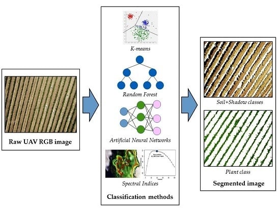
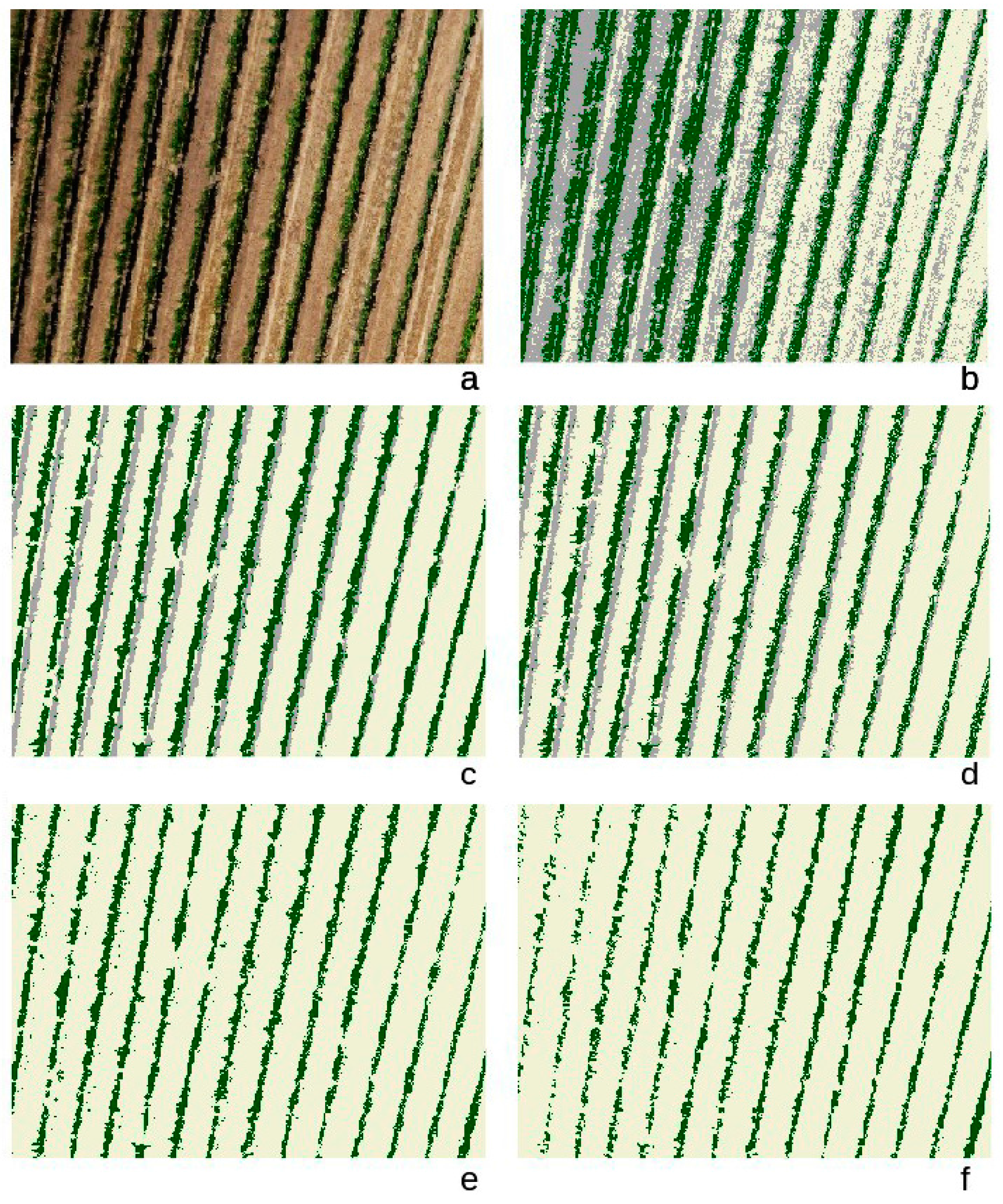
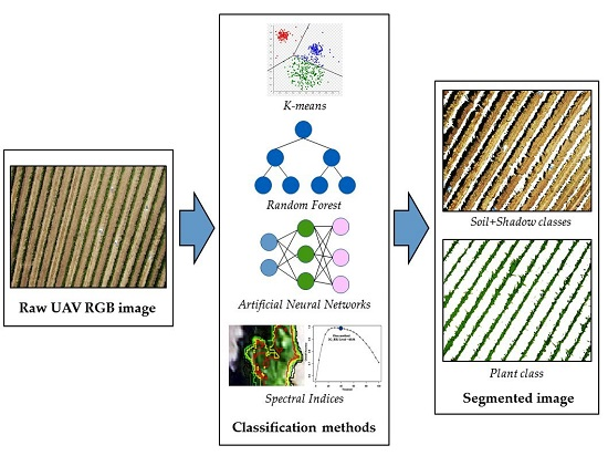
2.3. Description of the Classification Models

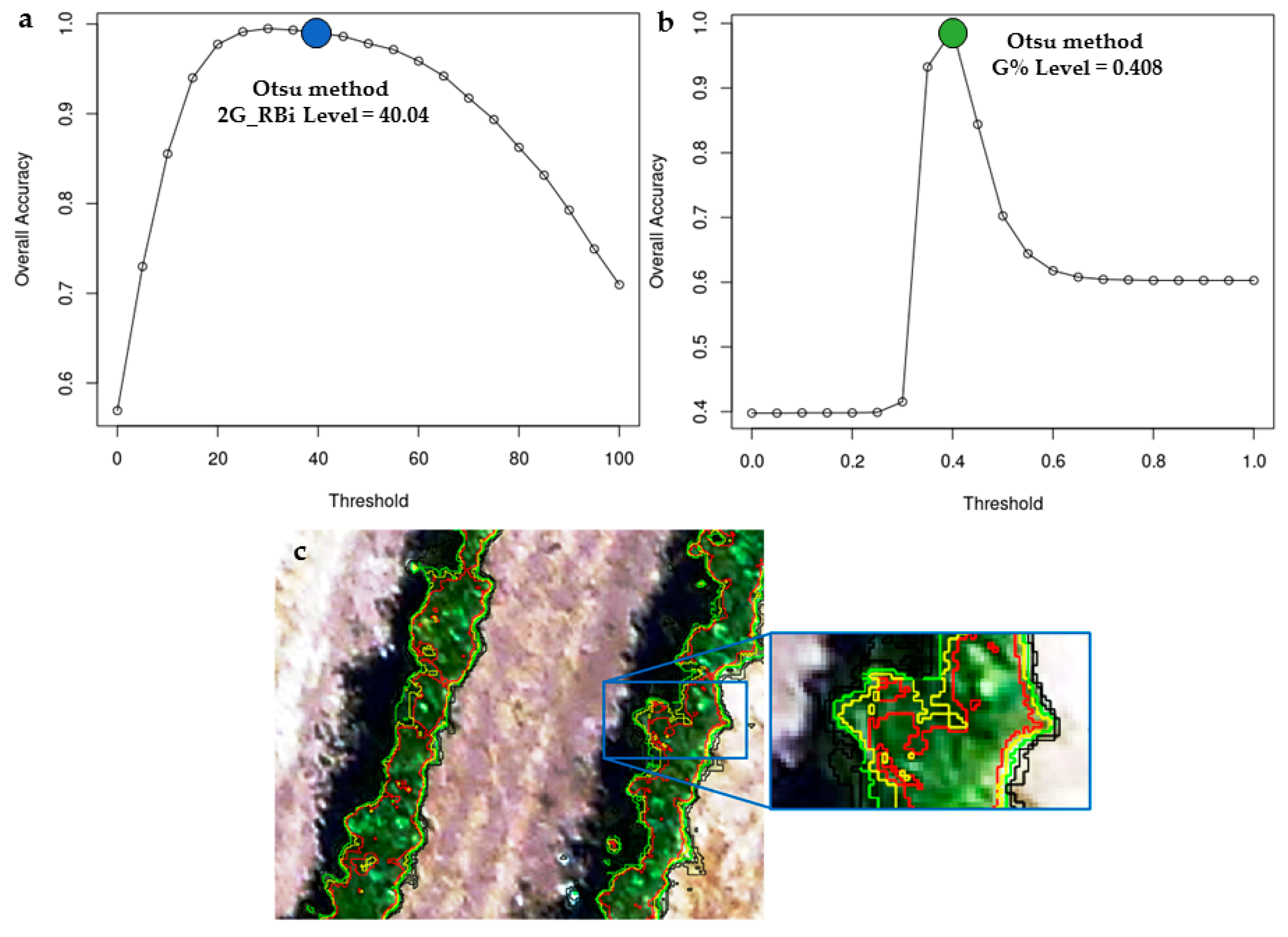
2.3.1. Spectral Indices as Classification Methods

For calculating the spectral indices (SI), color channel information (Digital Numbers; DNs) was extracted from the JPEG files for each of the three separate color channels (RDN, GDN, and BDN). The difference index (2G_RBi), was computed as proposed in [22] as the difference of the divergence of both red from green and blue from green, using absolute channel brightness (Equation (1)):
2 G _ R B i = 2 · G D N ( R D N + B D N )
Also, the Green percentage index (G%) was calculated as follows:
G % = G D N R D N + G D N + B D N
For using the SI as a classification method, it is necessary to have threshold values. These values were obtained by applying the Otsu’s multilevel thresholding method (MOM) implemented in Matlab (Matlab R2014a, Mathworks, Natick, MA, USA) considering one threshold i.e., two classes: Plant and Soil. This method finds the optimal thresholds by maximizing the weighted sum of between-class variances [23,24,25].

2.3.2. K-Means Clustering Method

K-means is a simple, unsupervised and clustering method that classifies the input data objects into multiple classes based on their inherent distance from each other [26]. K-means is generally used to determine the natural grouping of pixels present in an image. This method is attractive in practice because it is straightforward and it is generally very fast. K-means partitions the input data set into k clusters defined by the user.
The clustering algorithm assumes that a vector space is formed from the data features and tries to identify natural clustering of the data features. Each cluster is represented by an adaptively changing center (also called cluster center), starting from some initial values named seed-points. K-means clustering computes the distances between the inputs (also called input data points) and centers, and assigns inputs to the nearest center. The method follows a simple and easy procedure to classify a given data set through a certain number of clusters fixed a priori. The main idea is to define k centroids, one for each cluster. The initial locations of the centroids should be chosen with care because different initial locations can yield differing clustering results. Ideally the initial locations should be chosen to ensure that they are located as far away as possible from each other [26]. This algorithm assigns each pixel to one of the k clusters defined previously. Following this, every pixel must be assigned to a class. This was done comparing ground true data with the cluster. The cluster with the best coincidence with the plants locations is assigned to the Plant class. The one with the best coincidence with the soil, is assigned to the Soil class. The K-means clustering method was implemented using kmeans function from the stat package [27] of the Comprehensive R Archive Network (CRAN).
For this study, two different models were estimated using the K-means method. The first using the R, G and B channels as input data (K-means); and the second using the R, G, B channels, and the SI (from Section 2.3.1) as input data (K-means.ex). In both models, the maximum number of iterations allowed was limited to 50, and the number of clusters was set to 3. The algorithm used in both models was the one presented in [28]. The initial location of the centroids was chosen randomly using 10 random sets. The details and parameters used for the model are shown in Table 2.

2.3.3. Artificial Neural Networks

Artificial Neural Networks (ANN) are mathematical models inspired by the structure and behavior of the human brain. ANN are recognized as powerful and effective tools to solve complex dependencies that are difficult to analyze using other traditional statistical methods [29]. ANN are commonly used for classification in data science, grouping feature vectors into classes, allowing the analyst to input new data and find out which label fits best. Among the different types of ANN, the multilayer perceptron (MLP) is one of the most commonly used. It is constituted by multiple layers and the information is transferred from the input layer to the output layer (feed-forward). This kind of ANN is based on supervised learning (or “machine learning”), which relies on the use of input and output datasets (the “training” datasets) to iteratively change the weights until the simulated outputs are similar to the observed ones. To minimize the error, the algorithm employs the values of the error calculated in the previous iteration and then updates the weights. All numerical ANN calculations were performed using R package nnet [29], which constructs the standard single-hidden-layer neural network with neurons based on logistic function neurons.
In addition to nnet, the R package caret [30] was also used. This package helps with tuning the model parameters using intensive re-sampling with replacement in order to reduce uncertainty and then, choose the “optimal” model across these parameters. This optimization process in known as “bootstrap”, and the ANN generated by this process, as “bootstrap based artificial neural networks”. For this study, the parameters size and decay were optimized with a bootstrapping process. The size parameter represents the number of units in the hidden layer, and the decay parameter controls the weight decay in the optimization process. We tried different ANN with sizes ranging from 1 to 7, and decay s of: 0.0, 0.1 and 0.001. Two different models were trained, the first using the R, G, and B channels as input data (ANN), and the second using R, G, B, and the SI as input data (ANN.ex). The training dataset was composed of 672 manually selected samples. The details and parameters used for the model are shown in Table 2.

2.3.4. Random Forest

Decision trees are powerful and popular tools for classification and prediction. In this sense, two well-known ensemble methods are boosting (e.g., [31]) and bagging of classification trees [32]. In boosting, successive trees give extra weight to points incorrectly predicted by earlier predictors. In the end, a weighted vote is taken for prediction. In bagging, successive trees do not depend on earlier trees, each tree is independently constructed using a bootstrap sample of the data set. In the end, a simple majority vote is taken for prediction. In 2001, [33] proposed the Random Forest (RForest) method, which is an ensemble approach used for classification. The methodology includes construction of decision trees of the given training data, matching the test data with these and adding an additional layer of randomness to bagging. In addition to constructing each tree using a different bootstrap sample of the data, random forests change how the classification or regression trees are constructed. In standard trees, each node is split using the best split among all variables. In a random forest, each node is split using the best among a subset of predictors randomly chosen at that node. This somewhat counter-intuitive strategy turns out to perform very well compared to many other classifiers, including discriminant analysis, support vector machines, and neural networks and is robust against over-fitting [33,34].
In this study, the RForest method was implemented using randomForest package obtained from Comprehensive R Archive Network (CRAN) [35]. Two models were trained: the first using the R, G, and B channels as input data (RForest) and the second using those channels and the SI as input data (RForest.ex). The number of trees to grow was set to 500, the proximity was measured among the rows, and the importance of the predictors was assessed. These models were trained using the same training set as in the ANN (672 samples). The details and parameters used for the model are shown in Table 2.

2.4. Accuracy Assessment

A confusion matrix was used to assess the classification accuracy from independent validation samples. Kappa index, Overall Accuracy (OA), and Sensitivity were derived from confusion matrix to quantify the performance of classification methods using the R package caret. Independent validation samples were selected manually from RGB sample images for the six dates analyzed. The total number of validation samples for the Plant, Shadow, and Soil classes were 1500, 750, and 1500, respectively. The Sensitivity was estimated as the relationship between the samples predicted correctly as a class compared with the number of samples of that class, predicted correctly or incorrectly. The OA represents the percentage of samples predicted correctly. Finally, the Kappa statistic is a measure of the accuracy relative to what would be expected by chance. The latter is an excellent performance measure when the classes are highly unbalanced [36]. About 70% of the pixels of the images used in this study belong to the Soil class. This implies that a random classifier would predict the Soil class with a high accuracy. At the same time, between 20% and 30% of the pixels belong to the Plant class. So, predicting this class with a random classifier would predict the Plant class with a low accuracy.
Additionally, the relative contribution or relevance of each channel and index was calculated. For the ANN methods, the procedure was based on [37], which uses combinations of the absolute values of the weights. For the RForest methods, we used the mean decrease in accuracy as proposed in [32]. The relative contribution or relevance presented was normalized as a percentage, assigning a value of 100 to the most relevant channel/index.

3. Results

Threshold values for SI were obtained by applying the Otsu’s multilevel thresholding method. The obtained values were analyzed in terms of the OA with the validation samples for the Plant class. Figure 1a,b show the comparison between OA and threshold values obtained by the Otsu method for a selected flight in Veraison period (DOY29). For both SI, the threshold values obtained by Otsu method are very close to the optimum values indicated in the simulation carried out with the entire range of threshold values. Same results were obtained with all dates analyzed in this study. Furthermore, an example of visual interpretation of thresholding process of 2G_RBi for Plant class is presented in Figure 1c.
The parameters OA, Kappa index and Sensitivity for the different methods are presented in Table 3. The method with the best OA for the six dates analyzed is the spectral indices (2G_RBi) reaching an average value of 0.98. This method also has the best Kappa index (average value of 0.96). The second method with the best performance is the ANN (both configuration ANN and ANN.ex) reaching an average OA and Kappa index of 0.97 and 0.95, respectively (Table 3). One important characteristic of this method is that presents a high Sensitivity to detect the Plant, Soil, and Shadow classes. In the case of Sensitivity to detect the Plant class, ANN had average values of 0.94 and 0.95 for the basic and extended version, respectively. In the case of RForest method, OA values registered in the experiment were lower with average values of 0.87 and 0.94 for the basic and extended version, respectively. Additionally, for the machine learning methods, we measured the contribution of each input variable to the classification OA (Table 4). In the models that only used the R, G, and B channels as input data, the channels R and G were the variables which contributed more to the OA. In the extended methods using also the spectral indices, the major contributor to the OA was the G% for both cases (ANN.ex and RForest.ex) (Table 4).
The standard automatic method, K-means, with both configurations, performed poorly with average OA values of 0.64 for the extended version and 0.6 for basic version. This effect is clearer in the results of Kappa index, in which case the method presented very low average values of 0.39 for K-means and 0.46 for K-means extended. This indicates a limited performance for detecting the Plant class, which is corroborated by low Sensitivity for the Plant class, with average values of 0.27 for K-means and 0.24 for K-means extended.
Figure 2 shows the results of different classification methods using R, G, B channels and the spectral indices as input data. Spectral indices as classification methods do not allow to discriminate between Soil class and Shadow class (Figure 2e,f). On the other hand, the K-means method tends to confuse the Soil class with the Shadow class and the Plant class with the Shadow class (Figure 2b). The machine learning methods (ANN.ex and Rforest.ex) produced similar results (Figure 2c,d).

4. Discussion

4.1. Perspectives and General Study Limitations

The development of new techniques for UAV image analysis is an important aspect for PV, because today UAVs are rapidly replacing to other platforms for vineyard monitoring. The key strengths of UAV are the high spatial ground resolution and a reduced planning time, which allows for highly flexible and timely vineyard monitoring [15,38,39,40]. This study presents results using different classifications methods to detect and segment the vine canopy in ultra-high-resolution RGB imagery obtained from UAV. On very high spatial resolution images, the plantation and training patterns become distinguishable, providing great discrimination and characterization potentialities [39]. The potential utility of the presented study, is high, considering that the methodology was tested under standard commercial vineyard conditions (vines trained on VSP). Even though the study was limited to six UAV flights (from post-flowering to harvest) at a single vineyard site. Furthermore, the methodology presented as a case study for vineyards could be extrapolated to other sparse crops, where the effect of soil, shadows, and weeds need to be considered and eliminated from the analysis. Further validation in several vineyards, vine varieties, and other crop types is required to support stronger conclusions.
Recent studies have demonstrated that high-resolution RGB images obtained by low-cost cameras can be used to monitor spatial variability of vine biophysical parameters. [15] estimated the leaf area index (LAI) of a vineyard with a conventional digital camera (Canon PowerShot) mounted on a micro-UAV using the structure from motion (SfM) technique. In the same way, [16] estimated LAI of a vineyard using data from a hyperspectral camera (VNIR imaging sensor) and a low-cost standard RGB camera (GoPro Hero3) onboard a UAV system. In this study, the determination coefficient (r2) for the relationship between ground truth LAI and 2D GRVI map from the aerial RGB ortho-mosaic was 0.73.
To improve the evaluation of vineyard attributes from UAV images, automated tools are required to rapidly extract relevant information from canopy excluding the effect of soil and shadow. In this regard, [14] indicated that when the analyses were focused only on the cultivated areas, excluding ground and shadows, vegetation index maps change significantly.

4.2. Accuracy of Classification Methods

In this study, the methods analyzed had different performances for vine canopy extraction. Our results indicated that the standard and fully automatic method K-means did not have satisfactory performance when detecting the vine canopy. In general, K-means tended to detect two clusters inside of Soil class (Figure 2d), due to the effect of the differences in the image values inside of the Soil class, so Plant and Shadow classes ended up mixed in the same cluster. This generates a low sensitivity to the defined classes and low performance values (Table 3). This problem could be related to the use of three clusters for the classification of three classes. Using the same number of clusters as classes enables labeling the cluster based on the class with the majority of the samples that fall within a cluster. Some applications of K-means increase the number of clusters to improve the probability of generating a set of clusters that correspond to the classes. However, to obtain a predefined number of classes, it is necessary to make a reclassification process, mixing more than one cluster in one class. This involves an additional step and makes the method harder to automatize. On the other hand, in some specific cases (Flight 1, 3 and 4) the sensitivity detected for the Shadow class was high. In these cases, K-means overestimated the Shadow class. Therefore, all validation points were classified in this class (Sensitivity = 1). However, this does not imply that the K-means method has a good performance since for these cases, the Sensitivity for the Plant and Soil classes was low, resulting in low OA values from the method.
The method with the best performance in the detection of vine canopy was SI (2G_RBi), complemented with the Otsu method for thresholding. The classified image with this method can be used as a mask to crop the original image. The result of this process using 2G_RBi as classification method is shown in Figure 3. One of the main advantages in the use of SI as classification methods is that the process can be done without the need to use a specific software package to perform the calculations of the indices. Furthermore, when the SI method is complemented by Otsu method, it is possible to automatize the segmentation process. The threshold values obtained by Otsu method are stable in time and not dependent on other a priori information [24,25]. Additionally, this process does not have to be trained like ANN or RForest, so a training dataset is not needed. However, considering the performance pixel by pixel, the SI do not enable the Soil and Shadow classes to be discriminated (Figure 2b,c). The ANN and RForest methods produced satisfactory results, but these two methods need to be trained to achieve good accuracy. This means that a trained data set must be manually generated to calibrate the models. As well as this, these two methods had many different parameters that affect the performance of the model. In this sense, the bootstrapping algorithm proves to be very useful to find the optimal value of these parameters. [39], mentioned that the best result to discriminate between vine and non-vine was obtained when using the R channel. In our work, the R channel was the most discriminatory variable only for the ANN model. However, it was the second (Rforest and ANN.ex) or third (Rforest.ex) most contributing variable in the other models. The R channel was outperformed by the SI when they were used (ANN.ex and Rforest.ex) and by the G channel in the Rforest method (Table 4).
It is important to note that when the spectral indices were used as auxiliary input data for the other classification methods, the models performed better than using only the R, G, and B channels. This is especially notable in the case of the Random Forest where the improvement was in the order of 8% of the OA.
The analysis of different dates shows that the results of all methods were similar for all dates. The structure of the vineyard for the different dates was quite similar in terms of vegetation. A constant canopy shape was maintained during the growing season, especially after full bloom by the effect of the summer pruning practices and decreasing of the vegetative growth of the shoots from Veraison period. In the case of SI and machine learning methods, all dates presented high values of OA and Kappa index. Furthermore, the threshold values obtained by the Otsu method were stable during the experiment (Table 3), with low standard deviation values, 3.15 for 2G_RBi and 0.01 for G%.
Table 5 provides a summary of most recent studies related to vine canopy extraction. The results obtained in this study are similar in terms of accuracy to those obtained in other studies carried out with complex methods and more expensive input data (e.g., Near Infrared images). In the case of satellite images, the highest resolution panchromatic bands are around 50 cm. With these type of images, the detection of the canopy is limited by canopy size especially in high-quality vineyards trained on VSP which are managed to have low vigor canopies. When pixels are large in relation to the surfaces or objects, a large proportion of pixels are mixed as they include canopy, soil, and shadow especially at the edges. In this regard, cameras onboard UAVs can acquire ultra-high resolution (e.g., in this study we obtained RGB images with a resolution of 0.019 m·pixel−1 with flights at 60 m of altitude). Thereby, UAV images allow us to detect many details and vineyard features normally not visible in aerial or satellite imagery. The vine canopy detection implemented in our study is based on a pixel by pixel performance of the analyzed methods, considering the small variations from the different surfaces (Plant, Soil, and Shadow classes) included in the vineyard images.

5. Conclusions

Our results demonstrate that it is possible to perform an accurate segmentation of vine canopy from ultra-high resolution RGB images obtained by a UAV in clear sky conditions, using classification methods for standard conditions of vineyards trained on VSP without cover crops in the inter-row. The automatic K-means method with basic and extended configuration had the lowest performance among the studied methods. On the other hand, the machine learning methods (ANN and RForest) had a satisfactory performance, especially the ANN method, reaching an average overall accuracy value of 0.97. However, these methods need some level of human intervention for calibrating the model with a training data set. The SI complemented with the Otsu method for thresholding, had a high overall accuracy and performed very well in the detection of Plant class. This method is automatic and easy to apply since it does not need specific software to perform the calculations of the indices. Furthermore, the threshold values obtained by the Otsu method are stable, and not dependent on other a priori information. Complementary, the SI used as auxiliary input data for the other classification methods (ANN.ex and RForest.ex) improved their performance reaching overall accuracy values around 0.98 with high sensitivity values for the three classes (Plant, Soil, and Shadow). These classification methods could be used to derive information from RGB images like the fractional cover and monitoring the development of the vineyard.

Acknowledgments

This study was supported by the Chilean government through the project FONDECYT de Iniciación (#11130601) and by the Argentinian government through the projects INTA PNAGUA1133043 and PNAGUA1133042. We would like to express our gratitude to CITRA-Universidad de Talca (Samuel Ortega Farias) for logistic support, Daniel Sepulveda, Leopoldo Fonseca and Mauricio Zuñiga for technical assistance during flight campaigns.

Author Contributions

C. Poblete-Echeverría conceived and designed the experiments; M. Bardeen designed and built the UAV; C. Poblete-Echeverría and M. Bardeen gathered the data; G.F. Olmedo and B. Ingram designed the models and analyzed the data; C. Poblete-Echeverría and G.F. Olmedo wrote the paper.

Conflicts of Interest

The authors declare no conflict of interest.

References

  1. Proffitt, T.; Bramley, R.; Lamb, D.; Winter, E. Precision Viticulture: A New Era in Vineyard Management and Wine Production; Winetitles: Ashford, South Australia, 2006. [Google Scholar]
  2. Comba, L.; Gay, P.; Primicerio, J.; Aimonino, D.R. Vineyard detection from unmanned aerial systems images. Comput. Electron. Agric. 2015, 114, 78–87. [Google Scholar] [CrossRef]
  3. Bramley, R.G.V.; Lamb, D.W. Making sense of vineyard variability in Australia. Available online: http://www.cse.csiro.au/client_serv/resources/Bramley_Chile_Paper_h.pdf (accessed on 13 March 2017).
  4. Gutierrez-Rodriguez, M.; Escalante-Estrada, J.A.; Rodriguez-Gonzalez, M.T. Canopy Reflectance, Stomatal Conductance, and Yield of Phaseolus vulgaris L. and Phaseolus coccinues L. Under Saline Field Conditions. Int. J. Agric. Biol. 2005, 7, 491–494. [Google Scholar]
  5. Rouse, J.W., Jr.; Haas, R.H.; Schell, J.A.; Deering, D.W. Monitoring Vegetation Systems in the Great Plains with ERTS. NASA Spec. Publ. 1974, 351, 309–317. [Google Scholar]
  6. Huete, A.R. A soil-adjusted vegetation index (SAVI). Remote Sens. Environ. 1988, 25, 295–309. [Google Scholar] [CrossRef]
  7. Gitelson, A.A.; Kaufman, Y.J.; Merzlyak, M.N. Use of a green channel in remote sensing of global vegetation from EOS-MODIS. Remote Sens. Environ. 1996, 58, 289–298. [Google Scholar] [CrossRef]
  8. Bachmann, F.; Herbst, R.; Gebbers, R.; Hafner, V.V. Micro UAV based georeferenced orthophoto generation in VIS + NIR for precision agriculture. Available online: http://www.int-arch-photogramm-remote-sens-spatial-inf-sci.net/XL-1-W2/11/2013/isprsarchives-XL-1-W2-11-2013.pdf (accessed on 13 March 2017).
  9. Smit, J.L.; Sithole, G.; Strever, A.E. Vine signal extraction—An application of remote sensing in precision viticulture. S. Afr. J. Enol. Vitic. 2010, 31, 65–74. [Google Scholar] [CrossRef]
  10. Hall, A.; Louis, J.; Lamb, D. Characterising and mapping vineyard canopy using high-spatial-resolution aerial multispectral images. Comput. Geosci. 2003, 29, 813–822. [Google Scholar] [CrossRef]
  11. Nebiker, S.; Annen, A.; Scherrer, M.; Oesch, D. A light-weight multispectral sensor for micro UAV—Opportunities for very high resolution airborne remote sensing. Int. Arch. Photogramm. Remote Sens. Spat. Inf. Sci. 2008, XXXVII, 1193–1200. [Google Scholar]
  12. Zhang, C.; Kovacs, J.M. The application of small unmanned aerial systems for precision agriculture: A review. Precis. Agric. 2012, 13, 693–712. [Google Scholar] [CrossRef]
  13. Feng, Q.; Liu, J.; Gong, J. UAV Remote Sensing for Urban Vegetation Mapping Using Random Forest and Texture Analysis. Remote Sens. 2015, 7, 1074–1094. [Google Scholar] [CrossRef]
  14. Candiago, S.; Remondino, F.; De Giglio, M.; Dubbini, M.; Gattelli, M. Evaluating Multispectral Images and Vegetation Indices for Precision Farming Applications from UAV Images. Remote Sens. 2015, 7, 4026–4047. [Google Scholar] [CrossRef]
  15. Mathews, A.J.; Jensen, J.L.R. Visualizing and quantifying vineyard canopy LAI using an unmanned aerial vehicle (UAV) collected high density structure from motion point cloud. Remote Sens. 2013, 5, 2164–2183. [Google Scholar] [CrossRef]
  16. Kalisperakis, I.; Stentoumis, C.; Grammatikopoulos, L.; Karantzalos, K. Leaf area index estimation in vineyards from UAV hyperspectral data, 2D image mosaics and 3D canopy surface models. Int. Arch. Photogramm. Remote Sens. Spat. Inf. Sci.-ISPRS Arch. 2015, 40, 299–303. [Google Scholar] [CrossRef]
  17. Rabatel, G.; Delenne, C.; Deshayes, M. A non-supervised approach using Gabor filters for vine-plot detection in aerial images. Comput. Electron. Agric. 2008, 62, 159–168. [Google Scholar] [CrossRef]
  18. Nolan, A.P.; Park, S.; Fuentes, S.; Ryu, D.; Chung, H. Automated detection and segmentation of vine rows using high resolution UAS imagery in a commercial vineyard. In Proceedings of the 21st International Congress on Modelling and Simulation, Gold Coast, Australia, 29 November–4 December 2015; pp. 1406–1412.
  19. Ranchin, T.; Naert, B.; Albuisson, M.; Boyer, G.; Astrand, P. An automatic method for vine detection in airborne imagery using wavelet transform and multiresolution analysis. Photogramm. Eng. Remote Sens. 2001, 67, 91–98. [Google Scholar]
  20. Wassenaar, T.; Robbez-Masson, J.; Andrieux, P.; Baret, F. Vineyard identification and description of spatial crop structure by per-field frequency analysis. Int. J. Remote Sens. 2002, 23, 3311–3325. [Google Scholar] [CrossRef]
  21. Puletti, N.; Perria, R.; Storchi, P. Unsupervised classification of very high remotely sensed images for grapevine rows detection. Eur. J. Remote Sens. 2014, 47, 45–54. [Google Scholar] [CrossRef]
  22. Richardson, A.D.; Jenkins, J.P.; Braswell, B.H.; Hollinger, D.Y.; Ollinger, S.V.; Smith, M.L. Use of digital webcam images to track spring green-up in a deciduous broadleaf forest. Oecologia 2007, 152, 323–334. [Google Scholar] [CrossRef] [PubMed]
  23. Otsu, N. A Threshold Selection Method from Gray-Level Histograms. IEEE Trans. Syst. Man Cybern. 1979, 9, 62–66. [Google Scholar] [CrossRef]
  24. Liao, P.S.; Chen, T.S.; Chung, P.C. A fast algorithm for multilevel thresholding. J. Inf. Sci. Eng. 2001, 17, 713–727. [Google Scholar]
  25. Huang, D.Y.; Lin, T.W.; Hu, W.C. Automatic multilevel thresholding based on two-stage Otsu’s method with cluster determination by valley estimation. Int. J. Innov. Comput. Inf. Control 2011, 7, 5631–5644. [Google Scholar]
  26. Hunag, M.-C.; Wu, J.; Cang, J.; Yang, D. An Efficient k-Means Clustering Algorithm Using Simple Partitioning. J. Inf. Sci. Eng. 2005, 1177, 1157–1177. [Google Scholar]
  27. R Core Team R: A Language and Environment for Statistical Computing. R Foundation for Statistical Computing. Vienna, Austria, 2015. Available online: https://www.R-project.org/ (accessed on 15 March 2017).
  28. Lloyd, S.P. Least squares quantization in PCM. IEEE Trans. Inf. Theory 1982, 28, 128–137. [Google Scholar] [CrossRef]
  29. Venables, W.N.; Ripley, B.D. Modern Applied Statistics with S, 4th ed.; Springer: New York, NY, USA, 2002. [Google Scholar]
  30. Shapire, R.; Freund, Y.; Bartlett, P.; Lee, W.S. Boosting the Margin: A New Explanation for the Effectiveness of Voting Methods. Ann. Stat. 1998, 26, 1651–1686. [Google Scholar] [CrossRef]
  31. Breiman, L. Bagging predictors. Mach. Learn. 1996, 24, 123–140. [Google Scholar] [CrossRef]
  32. Breiman, L. Random forests. Mach. Learn. 2001, 45, 5–32. [Google Scholar] [CrossRef]
  33. Cutler, D.R.; Edwards, T.C.; Beard, K.H.; Cutler, A.; Hess, K.T.; Gibson, J.; Lawler, J.J. Random Forests for Classification in Ecology. Ecology 2007, 88, 2783–2792. [Google Scholar] [CrossRef] [PubMed]
  34. Liaw, A.; Wiener, M. Classification and Regression by Random Forest. R News 2002, 2, 18–22. [Google Scholar]
  35. Kuhn, M. Building Predictive Models in R Using the caret Package. J. Stat. Softw. 2008, 28, 1–26. [Google Scholar] [CrossRef]
  36. Baluja, J.; Diago, M.P.; Balda, P.; Zorer, R.; Meggio, F.; Morales, F.; Tardaguila, J. Assessment of vineyard water status variability by thermal and multispectral imagery using an unmanned aerial vehicle (UAV). Irrig. Sci. 2012, 30, 511–522. [Google Scholar] [CrossRef]
  37. Gevrey, M.; Dimopoulos, I.; Lek, S. Review and comparison of methods to study the contribution of variables in artificial neural network models. Ecol. Modell. 2003, 160, 249–264. [Google Scholar] [CrossRef]
  38. Mathews, A.J. A Practical UAV Remote Sensing Methodology to Generate Multispectral Orthophotos for Vineyards: Estimation of Spectral Reflectance. Int. J. Appl. Geospatial Res. 2015, 6, 65–87. [Google Scholar] [CrossRef]
  39. Delenne, C.; Durrieu, S.; Rabatel, G.; Deshayes, M. From pixel to vine parcel: A complete methodology for vineyard delineation and characterization using remote-sensing data. Comput. Electron. Agric. 2010, 70, 78–83. [Google Scholar] [CrossRef] [Green Version]
  40. Matese, A.; Toscano, P.; Di Gennaro, S.F.; Genesio, L.; Vaccari, F.P.; Primicerio, J.; Belli, C.; Zaldei, A.; Bianconi, R.; Gioli, B. Intercomparison of UAV, aircraft and satellite remote sensing platforms for precision viticulture. Remote Sens. 2015, 7, 2971–2990. [Google Scholar] [CrossRef]
  41. Karakizi, C.; Oikonomou, M.; Karantzalos, K. Vineyard detection and vine variety discrimination from very high resolution satellite data. Remote Sens. 2016, 8, 1–25. [Google Scholar] [CrossRef]
Figure 1. Example of the comparison between overall accuracy and threshold values for Spectral indices. (a) Difference index (2G_RBi); (b) Green percentage index (G%) and (c) Visual interpretation of thresholding process of 2G_RBi for Plant class. Values below 40 are shown in black, equal to 40 in green, 50 in yellow and 60 in red.
Remotesensing 09 00268 g001
Figure 2. Classification results for the different methods using R, G, B channels and the spectral indices as input data. In green plant class, beige: soil class and dark gray: shadow class. (a) original image; (b) K-means.ex; (c) ANN.ex; (d) RForest.ex; (e) G% and (f) 2G_RBi.
Remotesensing 09 00268 g002
Figure 3. UAV image masked using the result of the 2G_RBi classification method.
Remotesensing 09 00268 g003
Table 1. Unmanned aerial vehicle (UAV) specifications.
CharacteristicDescription
TypeQuadcopter
DimensionsDiameter 100 cm, height 45 cm
Weight5.4 kg with batteries (maximum weight on fly 9.0 kg)
Engine power4 multirotor motors × 250 W gearless brushless motors powered by a 14.8 V battery
Auto pilotHKPilot Mega 2.7
MaterialCarbon with delrin inserts
PayloadApproximately, 3.0 kg
Flight modeAutomatic with waypoint or based on radio control
EnduranceApproximately, 21 min (hovering flight time) and 18 min (acquisition flight time)
Ground Control Station8-channels, UHF modem, telemetry for real-time flight control
Onboard imaging sensorConventional RGB camera
Table 2. Details of the predictors, training samples and parameters used in K-means, Artificial neural network, and Random Forest methods.
MethodPredictorsTraining SamplesParameters
K-meansR, G, B-3 centers, 50 max iterations
K-means.exR, G, B, G%, 2G_RBi-3 centers, 50 max iterations
ANNR, G, B672size = 4, decay = 0.1
ANN.exR, G, B, G%, 2G_RBi672size = 5, decay = 0.1
RForestR, G, B672trees = 500
RForest.exR, G, B, G%, 2G_RBi672trees = 500
Table 3. Performance of the different classification methods.
MethodFlight1 DOY315Flight2 DOY22Flight3 DOY29Flight4 DOY63Flight5 DOY72Flight6 DOY78**Avg.
Overall Accuracy (Kappa Index)
* G%0.98 (0.98)0.96 (0.91)0.98 (0.97)0.94 (0.88)0.97 (0.93)0.93 (0.85)0.96 (0.92)
* 2G_RBi0.99 (0.98)0.97 (0.94)0.99 (0.98)0.97 (0.94)0.97 (0.94)0.98 (0.95)0.98 (0.96)
K-means0.81 (0.71)0.58 (0.35)0.53 (0.29)0.64 (0.47)0.54 (0.29)0.48 (0.21)0.60 (0.39)
K-means.ex0.96 (0.83)0.60 (0.38)0.55 (0.32)0.71 (0.57)0.56 (0.32)0.49 (0.22)0.64 (0.46)
ANN0.98 (0.97)0.96 (0.93)0.99 (0.98)0.96 (0.94)0.98 (0.97)0.93 (0.89)0.90 (0.95)
ANN.ex0.97 (0.96)0.96 (0.94)0.99 (0.99)0.96 (0.94)0.98 (0.98)0.94 (0.90)0.97 (0.95)
RForest0.96 (0.94)0.90 (0.84)0.88 (0.82)0.83 (0.73)0.90 (0.84)0.75 (0.60)0.87 (0.79)
RForest.ex0.97 (0.96)0.96 (0.94)0.98 (0.96)0.91 (0.86)0.95 (0.93)0.89 (0.83)0.94 (0.91)
Threshold Values Estimated Using the Otsu Method
* G%0.450.400.410.390.390.390.40
* 2G_RBi63.2737.2240.0434.4133.2831.0839.88
Sensitivity (Plant Class)
K-means0.020.000.550.420.070.560.27
K-means.ex0.000.000.380.460.230.390.24
ANN1.000.931.000.920.950.840.94
ANN.ex1.000.941.000.920.960.860.95
RForest0.940.850.810.650.820.670.79
RForest.ex0.980.920.950.780.880.730.87
Sensitivity (Shadow Class)
K-means0.000.000.001.000.000.000.17
K-means.ex1.000.001.000.000.000.000.33
ANN0.940.940.960.981.000.980.97
ANN.ex0.920.940.970.961.000.980.96
RForest0.940.780.800.840.860.420.77
RForest.ex0.940.960.971.001.001.000.98
Sensitivity (Soil Class)
K-means0.000.000.610.680.010.640.32
K-means.ex0.010.000.620.780.000.000.23
ANN0.980.991.001.001.001.000.99
ANN.ex0.970.991.001.001.000.990.99
RForest0.991.000.991.000.991.001.00
RForest.ex0.981.001.001.001.001.001.00
Table 4. Relative contribution to the overall accuracy of each input variable for the machine learning methods evaluated.
Input VariableANNANN.exRForestRForest.ex
R10052.9466.8655.45
G73.2101000
B045.31016.77
G%-100-100
2G_RBi-50.12-82.96
Table 5. Comparison of recent studies related to canopy vineyard segmentation.
MethodInput Data Spatial ResolutionBest Results from the Research StudyReference
Dynamic segmentation, Hough Space Clustering and Total Least Squares techniquesUAV. Near Infrared images5.6 cm ground resolutionAverage percentage of correctly detected vine-rows 95.13%[2]
Histogram filtering, Contour recognition, and Skeletonisation processUAV. Near Infrared images.4.0 cm ground resolutionAverage precision 0.971. Sensitivity 0.971.[18]
Object-based procedure and Ward’s Modified MethodAircraft. RGB images.30 cm ground resolutionOA for both methods 0.87[21]
Object-based procedureSatellite. Multispectral WorldView-2 images.50 cm Panchromatic imagery. 200 cm multispectral imagery.OA values above 96% for all datasets[41]

