Freeze/Thaw-Induced Deformation Monitoring and Assessment of the Slope in Permafrost Based on Terrestrial Laser Scanner and GNSS

Abstract

Most previous studies of the Qinghai-Tibet engineering corridor (QTEC) have focused on the impacts of climate change on thaw-induced slope failures, whereas few have considered freeze-induced slope failures. Terrestrial laser scanning was used in combination with global navigation satellite systems to monitor three-dimensional surface changes between 2014 and 2015 on the slope of permafrost in the QTEC, which experienced two thawing periods and a freezing period. Soil temperature and moisture sensors were also deployed at 11 depths to reveal the hydrological–thermal dynamics of the active layer. We analyzed scanned surface changes in the slope based on comparisons of multi-temporal point cloud data to determine how the hydrological–thermal process affected active layer deformation during freeze–thaw cycles, thereby comprehensively quantifying the surface deformation. During the two thawing periods, the major structure of the slope exhibited subsidence trends, whereas the major structure of the slope had an uplift trend in the freezing period. The seasonal subsidence trend was caused by thaw settlement and the seasonal uplift trend was probably due to frost heaving. This occurred mainly because the active layer and the upper permafrost underwent a phase transition due to heat transfer. The ground movements occurred approximately in the soil temperature conduction direction between the top of the soil and the permafrost table. The elevation deformation range was mainly −0.20 m to 0.20 m. Surface volume increases with heaving after freezing could have compensated for the loss of thawing twice and still led to the upward swelling of the slope. Thus, this type of slope in permafrost is dominated by frost heave. Deformation characteristics of the slope will support enhanced decision making regarding the implementation of remote sensing and hydrological–thermal measurement technologies to monitor changes in the slopes in permafrost adjacent to engineering corridors, thereby improving the understanding and assessment of hazards.

1. Introduction

Permafrost degradation, melting snow, and extreme weather events (heavy precipitation and hot summer) due to climate change will probably lead to slope failures, where landslides, soil creep, collapses, debris flows, and rockfalls may occur in permafrost regions [1,2]. In particular, continued warming will cause significant changes in the environment and the characteristics of frozen-soil engineering, which could accelerate the frequency of ground displacement hazards, including settling and heaving, as well as negatively impacting the infrastructure [3,4]. McRoberts and Morgenstern were the first to classify slope failures in permafrost, where they showed that thawing plays an important role in a wide range of landslide types associated with permafrost under climate change [5,6]. The instability of the slopes in permafrost regions can be classified into four main types, i.e., flow, slide, collapse, and creep [7,8]. In particular, the creep deformation of soils with slow-moving characteristics accounts for a high proportion of the movements in permafrost regions. Moreover, the movement of permafrost creep is upslope in winter due to freezing and downslope in summer because of thawing [9]. Thaw-induced slope failures in permafrost are affected mainly by the water and ice contents of the frozen soil [10], and most freeze-induced slope failures are caused by frost heaving [9]. There is concern that recent climate change is driving increases in permafrost slope failures, as well as possibly exacerbating this hazard further in the future [1]. The slopes in permafrost undergo very complicated physical, mechanical, and thermal changes during freeze–thaw cycles, where heat and water exchange occur with the near-surface atmosphere. In addition, the active layer and upper permafrost undergo a phase transition between solid and liquid during the heat transfer process. The climate in the Qinghai-Tibet Plateau (QTP) has been warming for the last decade, which has exacerbated surface deformation, thickened the active layers, and accelerated permafrost degradation. Crucially, permafrost degradation can cause slope failures, thereby threatening the integrity of roads, railways, bridges, pipelines, and other engineering constructions by causing damage such as fissuring, tilting, or even collapse [11,12]. Despite the increasing air temperature, studies of frozen disasters have not received much attention for nearly a decade.

Slope failures in permafrost regions have motivated the development of various monitoring techniques, such as total station, tension crack monitoring, microseismic monitoring technology, electrical resistivity tomography (ERT), terrestrial photogrammetric methods, global navigation satellite system (GNSS), slope stability radar, interferometric synthetic aperture radar (InSAR), and terrestrial laser scanning (TLS). Many studies have applied these monitoring techniques to slopes in permafrost. For example, steel rods spaced 10 m apart were deployed in transects transversal to the slope headwall to allow manual monitoring of slope retrogression in a permafrost region of the QTP, China [13]. Inclinometers were also used to detect changes in the downslope configuration of soils to obtain permafrost creep measurements in West Valley of Great Bear River, Canada [8,9]. Microseismic monitoring systems were installed at the Matterhorn (NW Alps) and nearby Lecco (Italy) to analyze the microseismic activity and facilitate rock slope stability investigations [14,15]. ERT measurements were employed to monitor mountain permafrost evolution in a seven-year study at Schilthorn, Swiss Alps [16]. Light detection and ranging (LiDAR) was deployed to assess rock slope failures in the permafrost high-mountain environments on the Monte Rosa east face [17,18]. InSAR technology was employed to measure surface deformation over permafrost in the QTP, North Slope of Alaska, USA, and the Mackenzie Valley, Canada [19,20,21,22,23,24]. TLS surveys have been conducted using three-dimensional (3D) laser scanners to describe and quantify the permafrost dynamics in an Arctic glacier basin, including rock slides and creeping [11,25], but the application of TLS in the QTP has been rare.

The increased air temperature and frequency of extreme weather events, and associated slope instabilities, mean that it is much more important to monitor permafrost evolution over the QTP at a high spatial-temporal resolution [16]. A large number of slopes in permafrost can be found along the Qinghai-Tibet engineering corridor (QTEC), which represents a potential geological hazard. In the present investigation, we performed a case study where 3D laser scanning measurement technology and GNSS were employed to map changes in order to estimate frost heave and thaw settlement on a slope in permafrost located in the QTEC, China. Most previous studies of the QTEC have focused on the impacts of climate change on thaw-induced slope failures, whereas few have considered freeze-induced slope failures. The QTEC is classified as a critical infrastructure and a passage that connects the inland region of China and the Tibetan Plateau. Successfully maintaining the corridor in non-dangerous, operational condition requires management strategies that employ quantitative and qualitative methods to analyze the past and present conditions that threaten human lives, vehicles, and infrastructure. Thus, freeze/thaw-induced slope deformation was monitored at the beginning and end of freezing and thawing between 2014 and 2015. Furthermore, we analyzed scanned surface changes in the slope based on comparisons of multi-temporal point clouds data to understand how hydrological–thermal changes affected the deformation process in the permafrost active layer during freeze–thaw cycles.

2. Materials and Methods

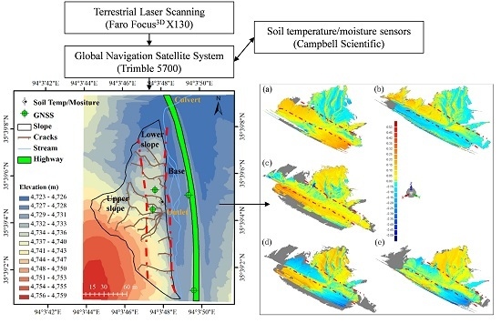
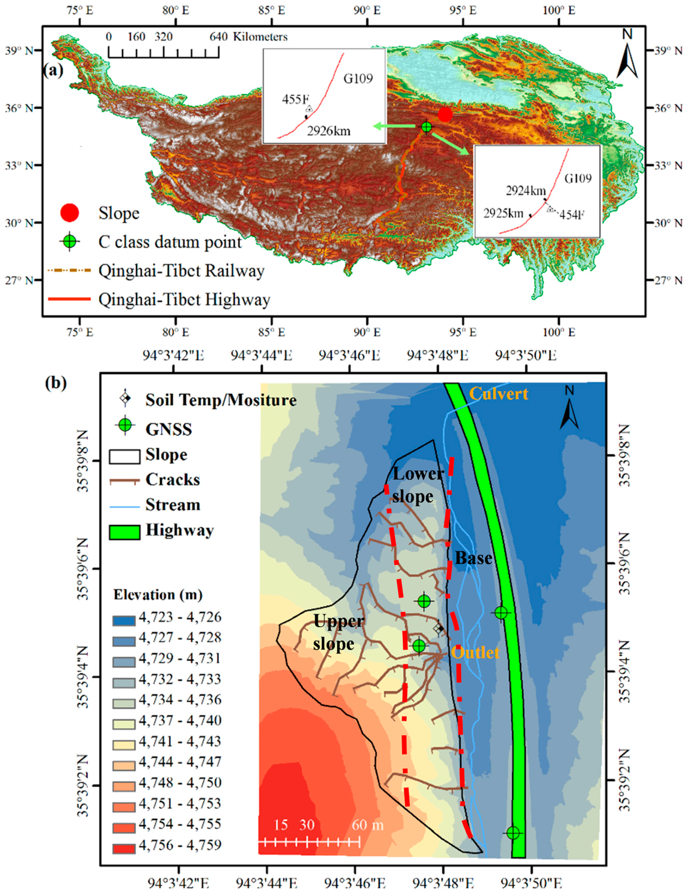
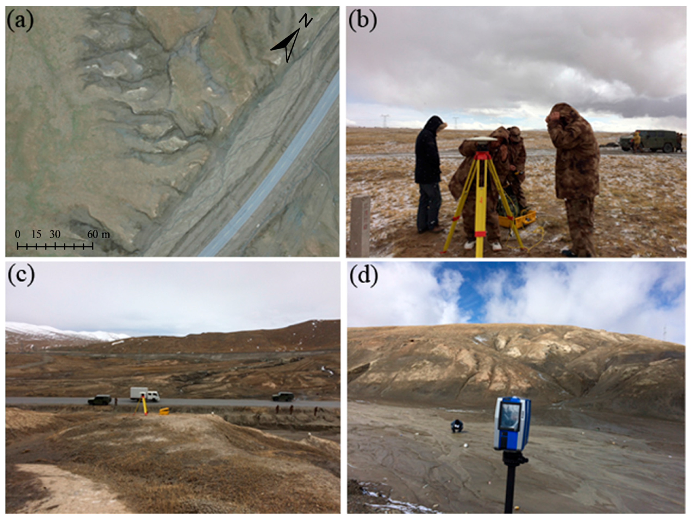
2.1. Study Site

The widespread distribution of permafrost-related slope failures in the QTP, especially along the QTEC, has long-term and highly damaging impacts on the ecosystem and engineering infrastructure. The QTEC stretches for about 1120 km from Geermu (Golmud) in Qinghai Province to Lhasa in the Tibet Autonomous Region. This naturally occurring north–south corridor in the central area of the QTP includes important engineering infrastructure, such as the Qinghai-Tibet railway (QTR), Qinghai-Tibet highway (QTH), gas and petroleum transmission pipeline, high-tension lines, and optical fiber cables [26]. The slope in the permafrost (94°03′46.00′′E, 35°39′4.00′′N, 4759 m a.s.l. in elevation) located around Kunlun Mountain Pass (KMP) in northern QTEC (Figure 1a) was selected as the study site, which is on the northwest side of the QTH near mileage K2897 and the QTR, where the distance is 8 m to 26 m from the QTH to the toe of the slope, and about 360 m from the QTR. High-tension lines are present on the adjacent slopes (~120 m northwest from the slope) and pipelines are also buried in the vicinity of the slope. The slope faces northeast, where the height of the slope is ~36 m, the mean slope is about 40°, and the total area is approximately 7620 m². The slope is subject to discontinuous island permafrost ground movements, including frost-heaving in winter and spring, and thawing in summer and fall. The beginning/end of the thawing/freezing seasons occurred on 28 April 2014 and 26 April 2015, and on 8 October 2014 and 12 October 2015.

The KMP is located in the heart of the East Kunlun Mountains in the QTP, where thick sediments from the early Quaternary were deposited. Drilling data (94°3′18.00′′E, 35°39′28.80′′N) obtained in the KMP during 2009 and 2013 showed that the strata mainly comprised Tertiary lake deposits and the Q4apl. Drilling was conducted 1.09 km to the north of the slope. The sediments in this area differ in their lithology and soil fractions at different depths, where the sediment variation from the top of the soil to a depth of 150 m in order comprises: clay, loam, sandy loam, sand, sand gravel, gravelly soil, and bedrock [27]. The annual mean air temperature in KMP is −7.1 °C to −1.8 °C and the annual mean ground temperature is −3.2 °C to −2.4 °C. The temperature ranges from a mean monthly minimum of −28 °C in winter to a mean monthly maximum of 18 °C in summer. The annual mean precipitation is 300–500 mm and the precipitation occurs most frequently in May–September, which accounts for 80% of the annual precipitation, where the maximum precipitation occurs from July to August (Figure 2). Permafrost is ice-rich with an active layer thickness (ALT) of more than 3 m. The maximum depth of the underground ice is about 90 m. Near a borehole, temperature measurement data showed that the temperature at the top of the permafrost was −2.8 °C, the permafrost thickness was about 85–90 m, the temperature gradient inside the permafrost was 3.5 °C/100 m, and the geothermal gradient under the permafrost was 4.5 °C/100 m.

The slope can be divided into: (a) the upper slope; (b) the lower slope; and (c) the base. The areas of the three zones relative to the total area of the slope were 39%, 28%, and 33%, respectively (Figure 6). Streams comprised the watercourse between the slope and the QTH, through which the snow melt, rainfall, and melt water from the slope flowed in the summer, and they converged into the streams that scoured the base of the slope. Thus, fluvial erosion also caused slope deformation. The watercourse was on the depositional area of the slope. Most of the water from the slope, which falls as rain and snow, flowed into the watercourse as an overland flow, whereas less water infiltrated into the active layer, and even less into the ground water. Ground water could supply water to the active layer.

2.2. Instruments

TLS was performed using a FARO Focus^3D X130 3D laser scanner, which is a high speed 3D scanner for obtaining detailed measurement and 3D documentation. This scanner employs a laser to produce highly detailed 3D images of complex environments and geometries within minutes. The resulting image is an assembly of millions of points in color, which provide an exact digital reproduction of the current conditions [28,29,30]. The distance accuracy of the FARO Focus^3D X130 is up to ±2 mm, with a range from 0.6 m to 130 m, and noise reduction of 50%. Approximately 26 scans were made in order to create a 3D point cloud of the entire site, with more than 1.1 million points. The TLS scanner and six Trimble 5700 GNSS systems were deployed in the field area between May 2014 and October 2015, where the site was monitored four times with two thawing periods and a freezing period (Figure 3). The three freeze–thaw phases are referred to as “first thawing” (May 2014 to October 2014), “freezing” (October 2014 to May 2015), and “second thawing” (May 2015 to October 2015) in the following.

Two of the six GNSS systems were deployed at two data points (454F and 455F) based on the national geodetic control network (NGCN) for the China geodetic coordinate system 2000 (CGCS 2000) near K2925 on the QTH [31], where the distance was 28 km from the slope to the two datum points (Figure 1a). The CGCS 2000 was used and we employed GNSS measurements from scan positions supplemented with two other GNSS instruments as control points based on the QTH near the slope, with the other two GNSS points on the slope (Figure 1b). The CGCS 2000 combined all the scanner coordinate systems to obtain the whole object [32]. In order to register the single scans and produce merged scan data with a common coordinate system, registration reference targets were placed using a FARO laser scanner reference sphere set (six reference spheres) and a set of rectangular white and black calibration cardboards in visible positions throughout the study area. The spheres were placed in the same position as the GNSS control points. The 3D point cloud data included the slope and the base. The displacement responses of the selected points were traced through the XYZ coordinates, where Z was the elevation of the slope. A series of point clouds were scanned on the slope surface and used to monitor its movement, as well as to examine the topographical change in the slope, to determine how much displacement occurred by comparing points in the same XY locations, and to scan the slope at different times.

In addition, the soil temperature was measured in the active layer of the slope at 11 depths (1, 30, 63, 80, 100, 123, 140, 175, 205, 235, and 260 cm) using thermocouple sensors (105T, Campbell Scientific). The soil water contents were recorded with 11 time-domain reflectometer (TDR) probes (Model CS615-L, Campbell Scientific) at 11 depths (10, 20, 48, 74, 91, 110, 135, 157, 190, 220, 245, and 270 cm). Two years of soil data were acquired from 1 May 2014 to 30 September 2015. The active layer was dominated mainly by clay from the top of the soil to 270 cm, including wet silty clay with grassroots (0–50 cm), loose silty clay (50–120 cm), compacted clay (120–180 cm), saturated clay mud (180–230 cm), loosed silty clay with gravel (230–250 cm), and clay with thick underground ice (250–270 cm). Based on the soil profiles, we inferred that the permafrost type in the slope could be classified as ice-rich permafrost.

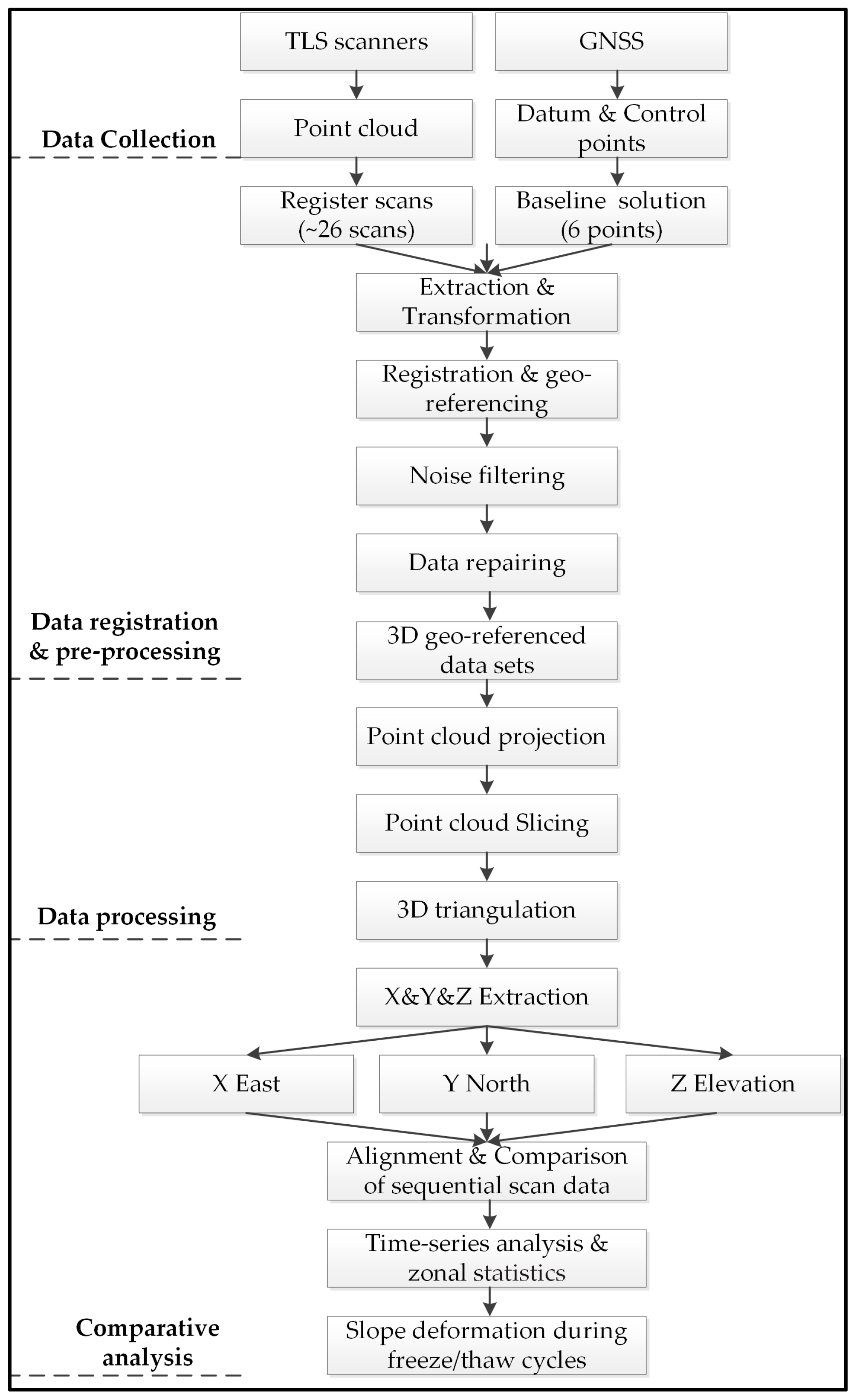
2.3. Processing on Time-Series TLS and GNSS

TLS is a laser-based technology that systematically measures the distance from the scanner to the imaging target in the 3D space, where millions of points represented the surface of the slope in permafrost. The device relies on a target that reflects the emitted laser beam to generate 3D point cloud data. The data were initially adjusted by GNSS programs from different GNSS base stations located throughout the slope. The GNSS solution was then combined with GNSS data inside TLS to generate geospatial data in the form of point clouds. The point cloud was then localized to a well-defined point throughout the slope to obtain the final geospatial value. The final values were then compared with the other TLS measurements. In order to retrieve the spatial-temporal dynamics of the slope deformation, we carried out time-series analysis based on 3D geo-referenced data sets. SCENE 5.0 and Geomagic studio 12 were adopted for processing these scanner data [33]. Our processing and analysis procedures can be divided into four stages (Figure 4): data collection, data registration and pre-processing, data processing, and comparative analysis. The point cloud data were collected from the four TLS with GNSS surveys. The reference targets were extracted from point cloud data for registration, and then these data were transformed to a common coordinate system. Data pre-processing is proposed to determine the scope of the slope, filter the noise points and repair data holes. The aim of 3D data post-processing was to use the registered point cloud data for fine mapping and 3D modeling. Projections and slices of point clouds are often used to simplify the data and to highlight the geometrical features of point clouds. Reality-based modeling uses registered point clouds to generate high-resolution polygons based on 3D triangulation. Multiple measurements at different times are necessary for assessing slope deformation. The changes mapped by the TLS on the slope were essentially used to examine the 3D surface topography based on direct spatial comparisons at different times. The displacement responses of selected points were traced through the XYZ coordinates, where Z was the elevation of the slope. A series of point clouds were scanned on the slope surface and used to monitor its movement, as well as for examining the topographic change of the slope, determining how much displacement occurred by comparing points in the same XY locations, and scanning the slope at different times. The point cloud datasets scanned on different dates had to be aligned using a combination of visually recognizable ground features and mathematical iterative best-fit algorithms. For the comparative analysis, the same datasets were divided into different parts of the slope using a slicing technique, so the freeze/thaw-induced deformation could be determined by zonal statistical analysis.

2.4. Data Uncertainties

TLS and GNSS are two different techniques, which can contribute in different ways to the investigation of a ground deformation phenomenon. The two data points of the GNSS network belonged to Class-C NGCN, where the coordinate values are based on the NGCN datum reference system. The 454F and 455F data points have much higher accuracy than the Continuously Operating Reference Stations (CORS) in China. Two data points and four control points were measured in advance, before starting TLS monitoring, and these GNSS instruments continue to collect measurements until the entire TLS scan was complete. GNSS was used to ensure that the orientation and registration of different 3D datasets employed a common coordinate system by measuring the ground data points and control points in TLS. Long-term monitoring of these data and control points also helped to improve the data accuracy for multiple scans. The use of 3D measurement technology provided data that could be transformed into a highly accurate reconstruction of the surface of the slope. The geometry of objects was maintained very precisely to record small changes, thereby producing a 3D image of the ground surface. These GNSS instruments collected ground reference points to ensure the highest geospatial accuracy, and they obtained strict ground control measurements for reference and calibrating the 3D laser scanner FARO. More importantly, the 3D laser scanner and GNSS acquired continuous high accuracy spatial deformation data from the slope, so we could compare the spatial changes in the slope’s surface over time via the GNSS network. Uncertainties are usually described as standard deviations (SDs), where it is assumed that the values follow a normal probability distribution [34]. The uncertainties of the TLS point clouds could be calculated using the reference targets. The SDs were computed from the adjusted coordinates for the TLS point cloud using least squares adjustment. The root mean square error (RMSE) was also calculated based on the differences between the positions of these targets measured by GNSS and their positions according to the TLS point cloud. The impacts on the point cloud data of the four TLS scanners were negligible because all the SD and RMSE values were less than 1 cm. Thus, the data accuracy met the needs for deformation measurement. The changeable climate of the QTEC is an important factor that affects TLS monitoring and data accuracy [35]. Foggy weather will also affect the accuracy of the instrument monitoring. Snow cover on the slope affected the comparative analysis at different time periods. Four TLS measurements were collected on the slope on days without snow cover. The vegetation was sparse on the slope and its height was low, where the vegetation returned at the beginning of May and then withered at the beginning of October. Therefore, the influence of snow and vegetation on TLS monitoring could be neglected. Furthermore, the TLS instrument consumed much more power in this alpine environment compared with the ordinary working state. Thus, there were data uncertainties and various different conditions, such as point uncertainties, surface uncertainties, 3D uncertainties, and comparative uncertainties. These uncertainties were complex and difficult to evaluate [36].

3. Permafrost Dynamics

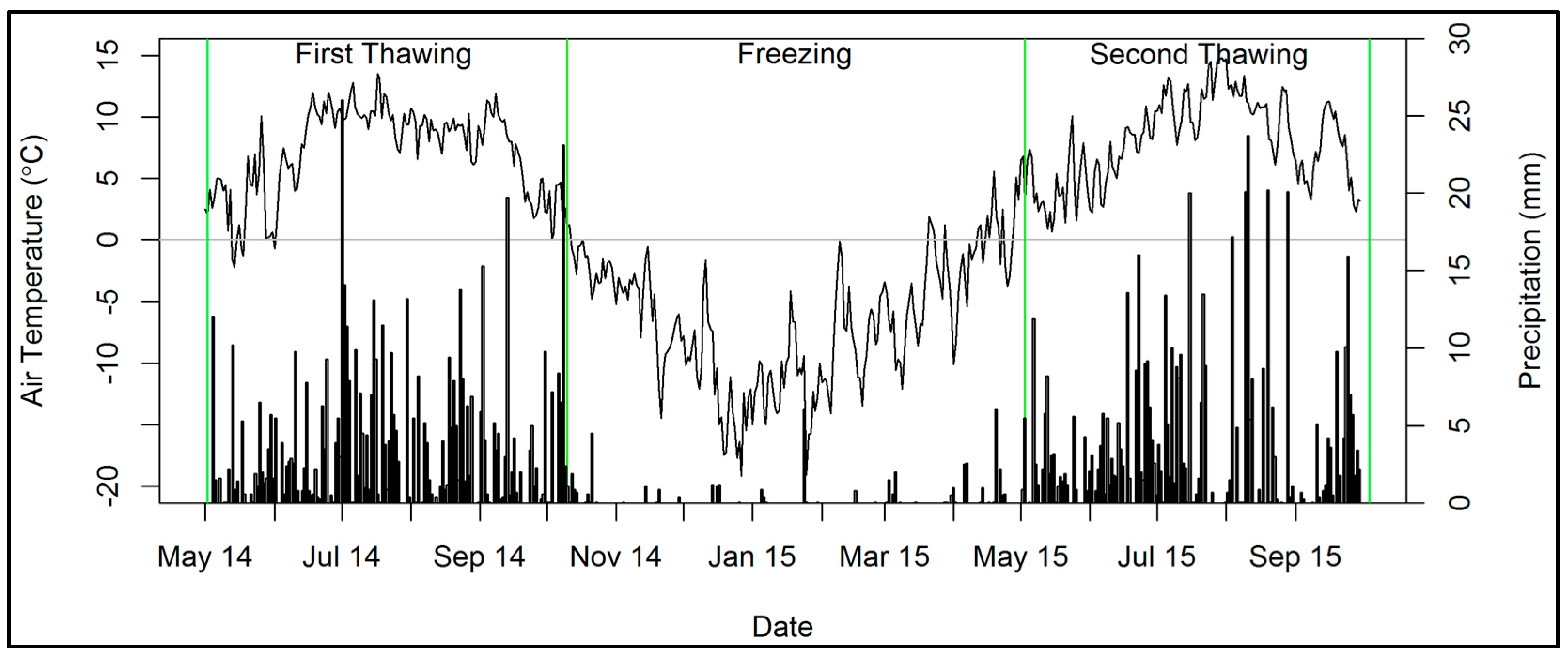
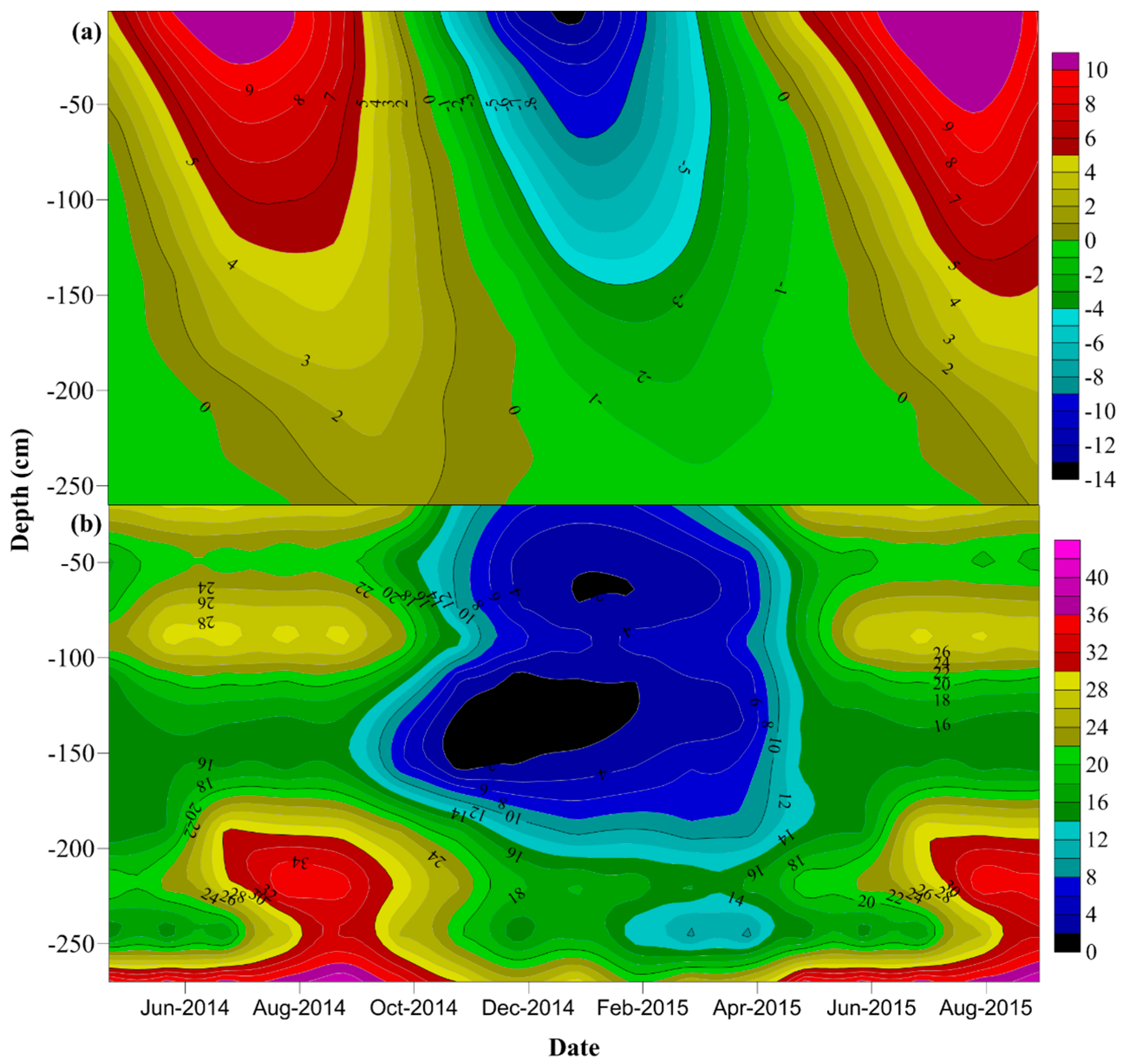
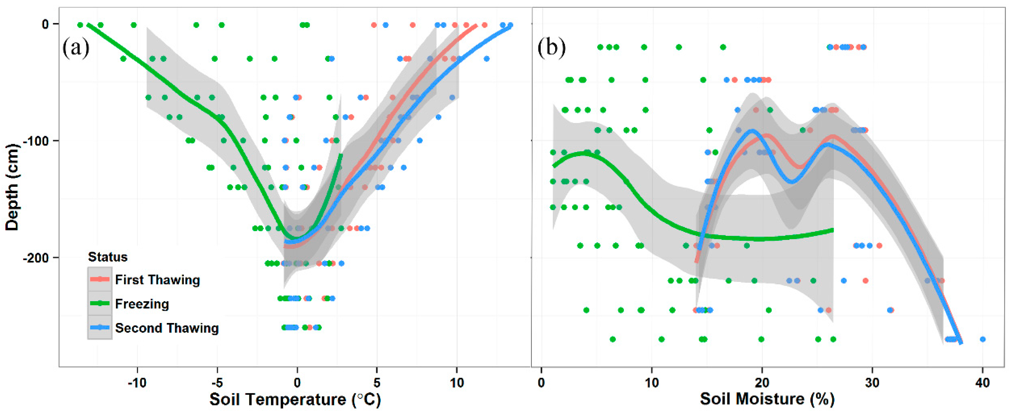
3.1. Hydrological–Thermal Dynamics

Permafrost is extremely vulnerable to climate change on different spatial and temporal scales. Changes in the hydrological–thermal dynamics of the ground due to permafrost thawing and freezing cause variations in energy exchange and hydrological processes between the atmosphere and ground surface [37,38]. The soil temperature and moisture content can indicate the hydrological–thermal dynamics of permafrost. We hypothesized that according to the slope deformation caused by permafrost thawing and freezing feedback, the changes in air temperature and precipitation would strongly influence the permafrost dynamics, thereby further affecting the slope stability in permafrost throughout the region.

The field monitoring results in Figure 5a show the soil temperature variations during freeze–thaw cycles. In early May, the active layer began to thaw from the surface to the permafrost table, and the active layer began to freeze bidirectionally in early October. The thawing of the active layer and the upper permafrost is a heat-absorbing process, which consumes large amounts of heat. With a constant state of heat transfer from the surface to the permafrost table, the thaw front migrated downward gradually. During the warming and thawing period, the soil temperature increased with the air temperature, where the soil temperature gradient in the active layer appear to decline from the top to the subsurface. As the heating process continued, the soil temperature gradient increased, where heat was transferred from the surface to the bottom, and the soil in the active layer begin to thaw from the surface. During the cooling and freezing period, soil heat was released into the atmosphere and the soil temperature declined continuously, so the soil began to freeze from the surface and the upper permafrost. Next, the active layer was in a completely frozen state and the soil underwent a sustained period of cooling. As the air cooled, the surface soil had a lower temperature than the subsoil, so the temperature gradient appeared to move upward. As the cooling continued, the soil temperature gradient gradually increased. The heat transfer from the active layer occurred from the bottom to the direction of the surface.

Figure 5b shows the soil moisture variations during freeze–thaw cycles. The active layer thawed completely, and the soil moisture contents were higher in the bottom and surface of the active layer, with higher soil moisture near the bottom and lower soil moisture in the middle. This was possibly attributable to the compacted clay near 150 cm, and the bottom of the active layer contained clay with thick underground ice. After the air warmed up sufficiently, the thaw front started to move down into the soil, and the underground ice in the active layer began to melt, where the contour lines of the soil moisture became dense again. As the thaw front moved downward slowly, the underground ice liquefied above the thaw front. The liquid water and snowmelt moved downward under the action of gravity. As the soil underwent the freezing process, the contour lines of the soil water content became more intensive and the soil water content changed sharply during this stage, where a large volume of liquid water froze. As the frost front moved downward gradually from the ground surface, the soil moisture moved upward gradually due to the effect of the soil temperature gradient. During the freezing period, most of the soil water was frozen into ice and only a small amount of unfrozen water moved upward under the temperature gradient.

3.2. Permafrost Indices

The permafrost model predicts the temporal and spatial variations in the thermal response of permafrost to changing climate conditions, as well as the earth surface and subsurface properties [39]. Permafrost indices can be computed using quantitative methods, such as analytical, numerical, or empirical functions, and models. Dozens of different indices have been used to evaluate the characteristics and dynamics of permafrost presence or absence, including the freezing/thawing depth, mean annual air temperature (MAAT), mean annual ground surface temperature (MAGST), and active layer thickness (ALT). These indices can be used to measure the intensity of freeze–thaw cycles and they can be combined with hydrological–thermal monitoring to analyze the slope deformation under the influence of freezing and thawing. The thawing depths can be computed using accumulated air degree-days, where thawing degree-days of air (°C-days) > 0 is the climatic index used widely in comparisons based on a variant of the Stefan solution [40,41,42] (Equation (1) and

Table 1. Climate and environmental variables for the KMP and the slope. The values comprise the parameters in 2014 followed by those in 2015.

Variable	Meaning	Unit	Value
ALT	Active layer thickness	m	3.26; 3.34
λt	Thermal conductivity of ground in thawed state	W/m°C	0.98
L	Latent heat of fusion	kJ/m3	1.17 × 105
γ	Dry bulk density	kg/m3	870
W	Soil water content in thawed state	%	24
Wu	Soil unfrozen water content in frozen state	%	5
Fa	Freezing degree-days for air	°C	1493; 1485
Fs	Freezing degree-days for ground	°C	1066; 999
Ta	Thawing degree-days for air	°C	1218; 1277
Ts	Thawing degree-days for ground	°C	2202; 2310
MAAT	Mean annual air temperature	°C	−0.75; −0.57
MAGST	Mean annual ground surface temperature (5 cm)	°C	3.11; 3.59

). We used the maximum thawing depth to quantify the permafrost dynamics. Thus, ALT was estimated as the maximum thawing depth. The maximum thawing depth in the permafrost zone can be simulated using the Stefan solution [43,44]. The surface deformation measured by TLS measurement is the total displacement and ALT can determine the range of soil layers where deformation occurs, thereby making it an important indicator of surface deformation. Definitions of symbols, and the climate and environmental factors are given in Table 1.

$$\mathrm{ALT}=\sqrt{\frac{2{\mathsf{\lambda }}_{\mathrm{t}}{\mathrm{T}}_{\mathrm{a}}}{{\mathrm{L}}_{\mathsf{\gamma }}(\mathrm{W}-{\mathrm{W}}_{\mathrm{u}})}}$$

(1)

The ALT definition of the maximum 0 °C isotherm penetration depth is directly related to soil temperature measurements [45,46]. ALT is estimated as the maximum thaw depth by linearly interpolating the soil temperature above and below the 0 °C isotherm (Figure 5a). According to borehole drilling and temperature records from 2014–2015, the values of T_a, T_s, MAAT, and MAGST were higher in 2015 than in 2014. By contrast, the freezing factors F_a and F_s exhibited systematic decreases in 2014–2015. The ALT estimates obtained from soil temperature measurements showed that the estimated ALT was higher in 2015 than that in 2014. Moreover, the ALT based on the 0 °C isotherm penetration depths or Stefan function was greater in 2015 than that in 2014. These results suggest that the permafrost continued to degrade because of the increasing air temperature.

4. Results

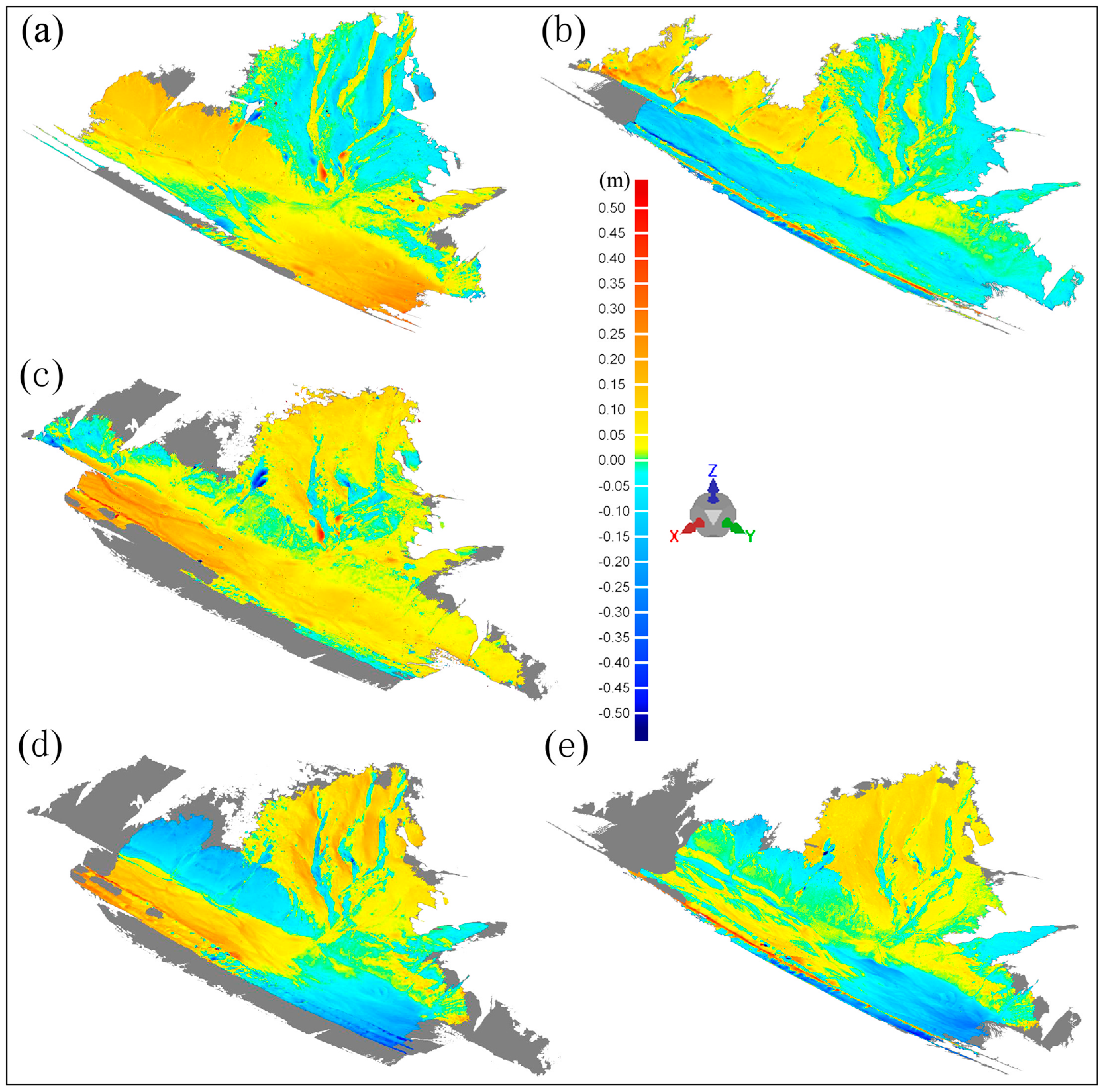
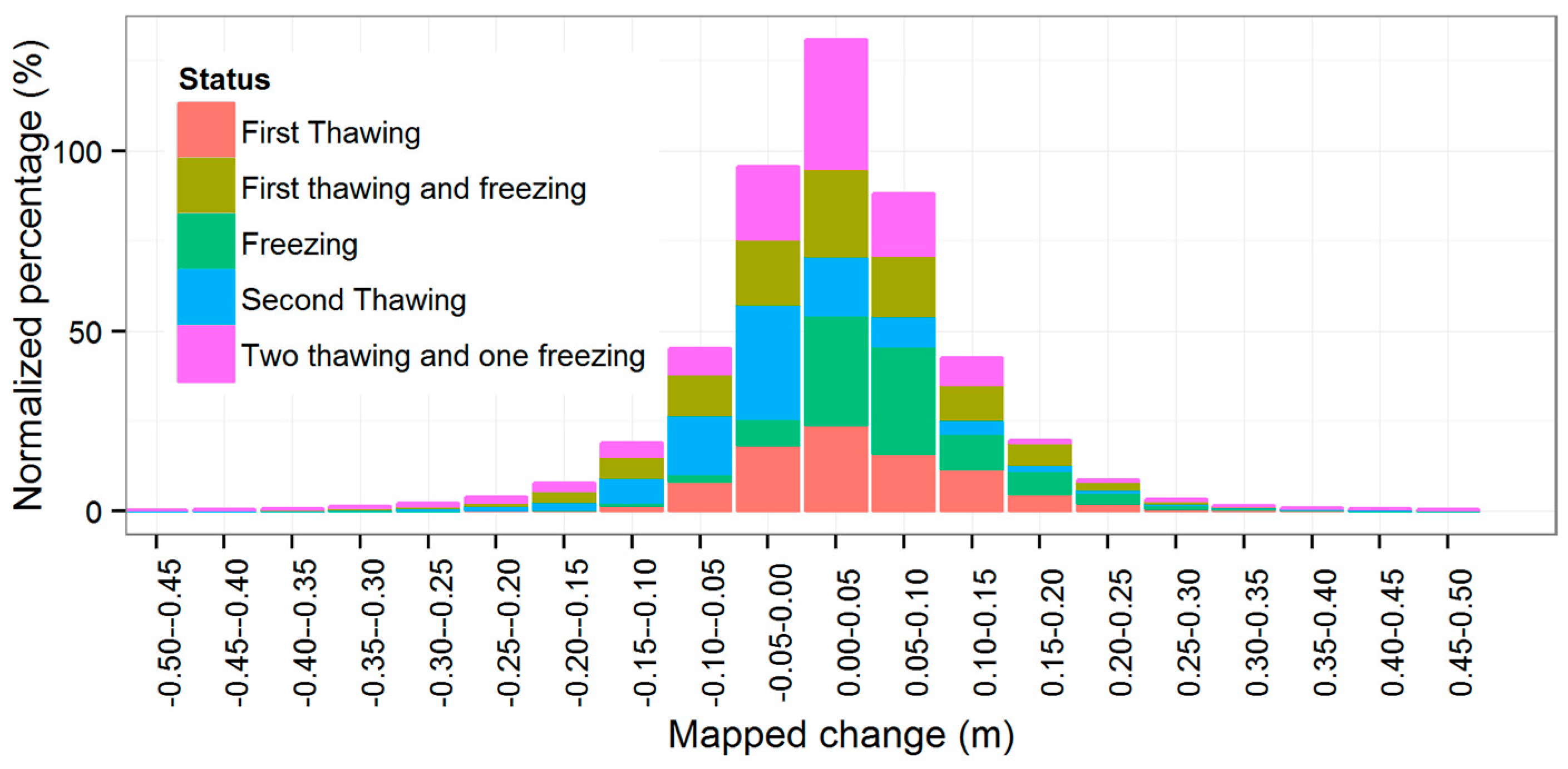
4.1. Deformation Analysis

4.1.1. Deformation Features during Thawing Periods

The 3D surface deformation results during the two thawing stages are compared in

Table 2. Comparison of the topographical change statistics.

Status	Time Span	Time Interval (days)	Mean Deviation (m)	Standard Deviation (m)	Data Points
First thawing	2 May 2014–10 October 2014	161	0.30	1.09	1,251,706
Freezing	10 October 2014–3 May 2015	205	0.20	1.39	1,291,356
Second thawing	3 May 2015–4 October 2015	154	0.46	0.98	1,248,325
First thawing and freezing	2 May 2014–3 May 2015	366	0.08	0.10	1,278,448
Two thawing and one freezing	2 May 2014–4 October 2015	520	0.07	0.22	1,279,706

and

Table 3. Standard deviation distributions for the topographical changes. Distribution percentages greater than 10% are highlighted in bold.

Status	Distribution Percentage (Standard Deviation of x, Unit of Measurement: %)
	x = −6	x = −5	x = −4	x = −3	x = −2	x = −1	x = 1	x = 2	x = 3	x = 4	x = 5	x = 6
First thawing	0.83	0.61	0.61	0.66	0.91	52.48	39.59	1.51	1.01	0.76	0.51	0.53
Freezing	1.03	0.66	0.78	0.81	0.60	4.53	89.51	0.51	0.43	0.35	0.31	0.48
Second thawing	0.33	0.26	0.50	0.63	1.07	76.68	16.66	0.88	0.73	0.65	0.54	1.07
First thawing and freezing	0.03	0.07	0.50	1.78	11.04	36.38	36.41	12.02	1.49	0.23	0.05	0.02
Two thawing and one freezing	0.41	0.07	0.10	0.17	2.09	37.23	58.30	1.18	0.11	0.07	0.05	0.23

, and the changes in elevation (Z) are shown in Figure 6a,b. The colored scale on the right-hand side (in meters) indicates the changes in elevation (Z) from −0.50 to +0.50 m. The changes in the terrain of the slope varied mainly from −0.05 m to 0 m in the two thawing stages. The proportional changes in terrain between −0.15 m and 0 m in the two thawing stages, with an interval of 0.05 m, were 6% and 12%, 28% and 36%, and 62% and 53%, respectively (Figure 7). The upper slope exhibited a subsidence trend during thawing conditions, where some deposits of soil occurred on the lower slope, with radial cracks as runoff gullies, and the base flowed during the first thawing. However, some of the fallen soil was scoured from the base during the second thawing stage. These deformations suggest that the upper slope exhibited a subsidence mode during thawing. We consider that the slope in the permafrost exhibited settlement during thawing periods. Part of the surface soil moved to the downslope of the lower slope, with radial cracks, and the base was the depositional area due to the action of gravity.

4.1.2. Deformation Features during Freezing Period

As shown in Table 2 and Table 3 and Figure 6c, the changes in elevation also ranged from 0.50 m to −0.50 m during the freezing stage. The changes in the elevation of the slope were mainly from 0 m to 0.10 m during one freezing period. The proportional changes in elevation between 0 m and 0.25 m, with an interval of 0.05 m, were 37%, 36%, 12%, 8%, and 4%, respectively (Figure 7). The upper slope exhibited an uplift trend during freezing conditions, where a small area of the lower slope and radial cracks in the slope exhibited a subsidence trend, although they only accounted for approximately 3% of the slope, which suggests that the major structure of the slope and the base comprised an upward swelling of the soil due to freezing. We consider that the slope in the permafrost was attributable to a frost heave phenomenon during the freezing period. Frost heave may also have occurred in most of the positions of the base.

4.1.3. Deformation Features during Thaw–Freeze Cycles

From May 2014 to October 2015, the slope in the permafrost underwent two thawing periods and one freezing period. During the two thawing periods, the major structure of the slope exhibited subsidence trends, but the major structure of the slope exhibited an uplift trend only in the single freezing period. It can be inferred that the surface volume was increased by heaving after freezing once due to the increased presence of ice as it grew toward the surface, which compensated for the loss of thawing twice, and there was still an upward swelling of the soil. Figure 6d,e compares the terrain during the thaw–freeze cycles after going through a freezing period, where regardless of whether there was one thawing or two thawing periods, the major structure of the slope still exhibited an uplift trend, which suggests that the upper slope still increased in size. The changes in the elevation of the slope were mainly from 0 m to 0.10 m during the two periods. The proportional changes in elevation between 0 m and 0.20 m in the two stages, with an interval of 0.05 m, were 40% and 57%, 28% and 27%, 16% and 12%, and 10% and 1%, respectively (Figure 7). The southern part and northern part of the base exhibited different deformation trends, i.e., uplift for the southern part and subsidence for the northern part. Despite the overall uplift of the slope, the lower slope and radial cracks in the slope showed some signs of slumping.

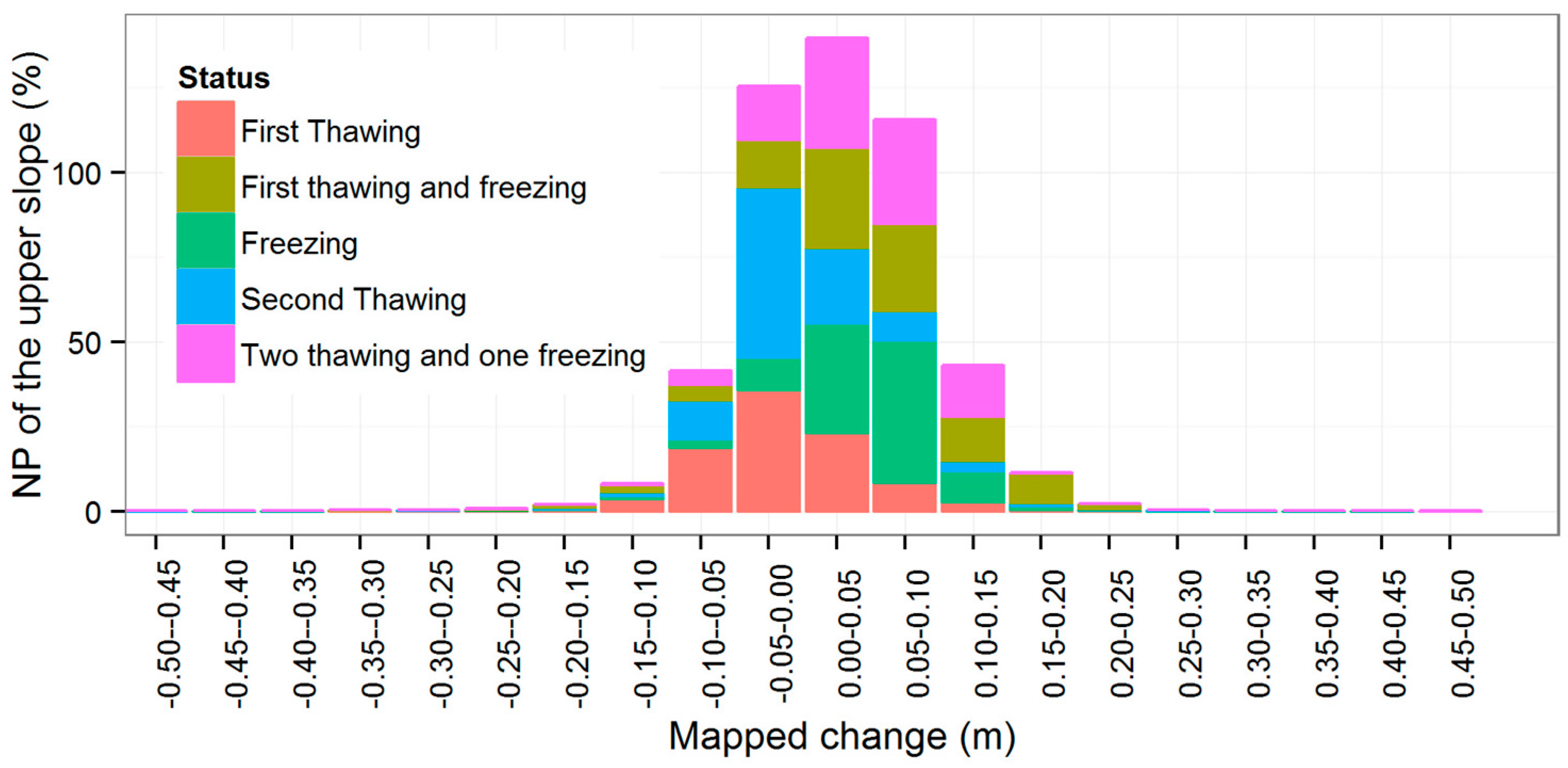
4.2. Zonal Deformation Analysis

4.2.1. Deformation Features of the Upper Slope

The upper slope zone comprised the slope body and radial cracks. The deformation of the slope body and radial cracks exhibited completely opposite trends during thawing and freezing. According to the zonal statistics, the deformations of the various zones and inside the zone of the slope had significant differences. Moreover, the soil movement in each zone could also be characterized based on the zonal statistics. During the two thawing periods, the slope body exhibited an even higher subsidence trend. The settlement percentages in terrain during the two thawing stages accounted for 60% and 64% of the total, respectively. Uplift of the radial cracks occurred due to slumping of the slope body. By contrast, the slope body exhibited an even higher uplift trend during the freezing period, where it accounted for 86% of the total. Regardless of whether there was one thawing or two thawing periods, after passing through a freezing period, more than 78% of the zone was still in a state of uplift (Figure 8,

Table 4. Comparison of the topographical change statistics for different zones of the slope.

Zones	Status	Mean Deviation (m)	Standard Deviation (m)	Data Points
Upper slope	First thawing	0.09	0.21	446,819
	Freezing	0.07	0.08	447,599
	Second thawing	0.06	0.12	507,888
	First thawing and freezing	0.08	0.08	522,739
	Two thawing and one freezing	0.07	0.11	522,464
Lower slope	First thawing	0.29	1.11	380,994
	Freezing	0.05	0.07	328,711
	Second thawing	0.07	0.13	387,682
	First thawing and freezing	0.04	0.07	396,478
	Two thawing and one freezing	0.03	0.05	395,680
Base	First thawing	0.31	1.19	430,174
	Freezing	0.30	1.27	458,191
	Second thawing	1.10	1.28	459,395
	First thawing and freezing	0.11	0.13	431,209
	Two thawing and one freezing	0.09	0.33	431,289

).

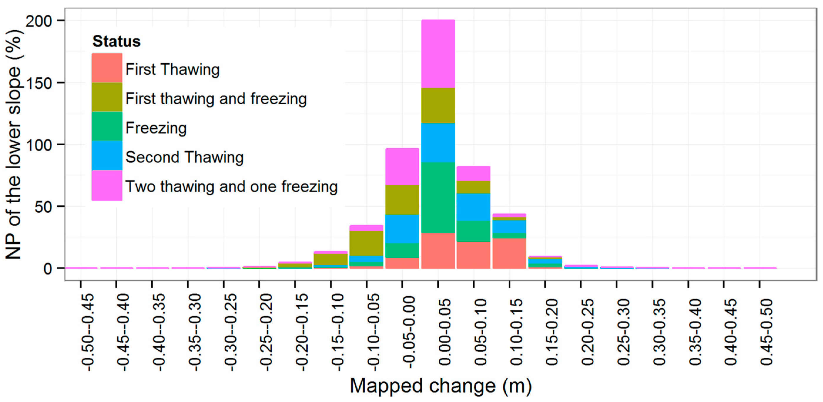
4.2.2. Deformation Features of the Lower Slope

The lower slope comprised the depositional area as well as the radial cracks of the upper slope. The lower slope mainly exhibited an uplift trend during thawing or freezing. The settlement percentages in the terrain during the two thawing stages and one freezing stage accounted for 13%, 30%, and 5% of the total, respectively. Regardless of whether there was one thawing or two thawing periods, after passing through a freezing period, more than 42% of the zone remained in a state of uplift (Figure 9, Table 4).

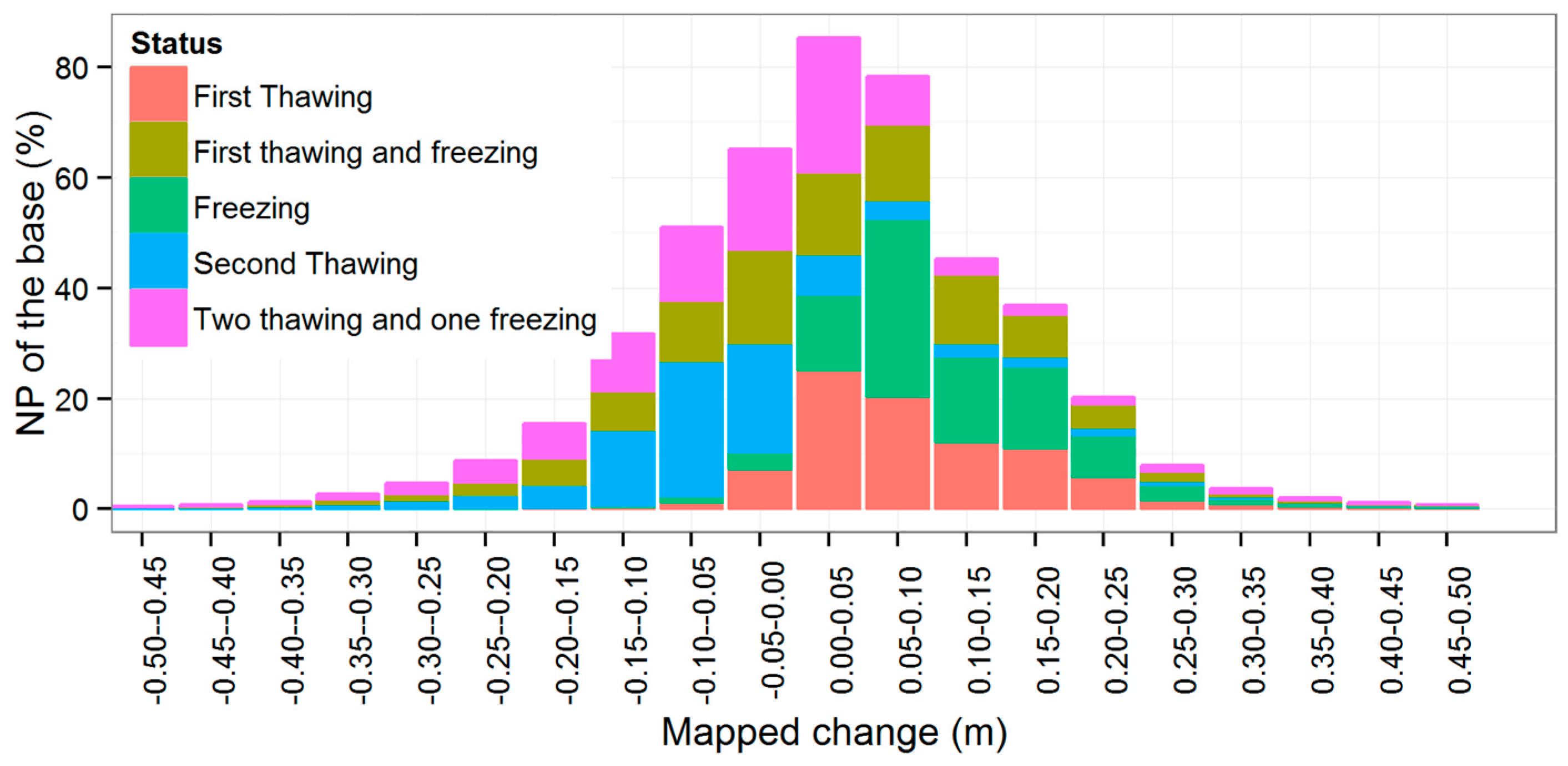
4.2.3. Deformation Features of the Base of Slope

The base comprised the depositional and erosion area, where sediment could be deposited by erosion and transport. The base deformation changed and the frost heave percentages in the terrain during the two thawing stages and one freezing stage accounted for 80%, 18%, and 89% of the total, respectively (Figure 10, Table 4). The normal distribution was narrowest for the lower slope, followed by the upper slope, and greatest for the base. These changes suggest that the base was affected more by the external environment (e.g., rainfall and overland flow) than the upper and lower slopes. The SD values for the base were more than 1 m during the two thawing and one freezing stage, but this does not mean that the uncertainty was greater, and the deformation was actually greater at the base of the slope. We suggest that the base was much more complex because it exhibited soil movements from the upper and lower slope regions in addition to settlement and heave. Moreover, there were many small streams at the base and it was located next to the Qinghai-Tibet Highway, so the impact of the external environment was greater.

5. Discussion

The amount of deformation depends on the water content and soil grains. Saturation of slopes by water is a primary cause of landslides. Differences in surface deformation in permafrost conditions involve the movement of fine-grained and ice-rich permafrost. In this study, we found a higher soil water content and thick underground ice near the permafrost table, where the active layer was dominated mainly by clay. The thaw front migrated downward gradually during the two thawing periods. Ice in the soil melted into liquid water, and the soil volume decreased because of the phase transition and the loss of soil water due to evaporation, as well as subsurface flow and seepage into the bottom [47]. The loss of soil water could have contributed to a reduction in volume. As expected, the slope deformation also exhibited a subsidence trend. Variations in energy control the seasonal dynamics of permafrost, where inter-annual variations govern annual fluctuations in thawing and the freezing depth of permafrost [48]. The results presented in Figure 5a show that the soil temperature in the second thawing exhibited more intense changes than those in the first thawing, while the ALT was deeper in the second thawing. Due to variations in energy, the surface changes on the slope were more significant in the second thawing than the first. In the two thawing phases, the slope generally exhibited subsidence. Settlement was caused by thawing of the ice-rich permafrost and subsequent thawing of underground ice in the slope. Most of the material lost from the slope in the thawing period was probably transferred into the underlying radial cracks and the base, and some was then washed into the base by rain or water because the elevation of the northern part of the base was lower. The lower slope was steeper than the upper slope and the direction of surface soil movement was markedly different. Most of the soil on the upper slope slid into the cracks, but a small amount fell to the lower slope, and most of the soil on the lower slope slid to the base of the slope. The deposits of soil in the cracks were directly transported to the base due to the actions of gravity and precipitation. Some of the soil at the base was washed into the culvert. In the freezing period, the surface soil on the slope was covered with snow, though the slope exhibited uplift, its stability was better than that in the thawing period, and the surface soil was less slippery.

Abundant water was present from a depth of 180 cm to the permafrost table. The permafrost table measured about 3.3 m and its recharge with ground water depended mainly on atmospheric precipitation. During the freezing period, the slope mainly exhibited heaving deformation. The adsorption force between soil particles and ice lenses under the action of negative pressure and vacuum could absorb the thawed water at the frozen fringe [49,50]. The study site had a high fines content with some clay layers and thick underground ice, which provided the internal conditions for frost heaving. Fine-grained soils such as clay and gravel are frost-susceptible. Winter may end before ice lenses grow sufficiently thick to cause harmful heaving, where they form segregated ice [50,51]. The frozen soil heaves because the formation of an ice lens pushes the soil grains relatively far apart, where the amount of frost heave is generally dependent on thawing, which favors the groundwater recharge. The temperature gradient is more significant if moisture can migrate into the permafrost due to the presence of bottom and a thaw zone, and these conditions are prone to frost heaving, which can result in land uplift and mound formation. The freezing period lasts for up to seven months in the KMP and a longer freezing period will allow frost heave to continue to develop, thereby forming a thicker ice layer, which does not melt in the warm season and this promotes the development of perennial frost heave. These changes may occur because of topographic variations in thaw–freeze cycles, including changes in hydrostatic and cryostatic pressure, and thermal stresses [52]. The frost front gradually migrated upward from the permafrost table in the freezing period. In addition, the soil water froze into solid ice and the soil volume increased. As expected, the slope deformation exhibited an uplift trend. Frost heave in alpine regions is often attributed to freezing and the volumetric expansion of water trapped within pores and cracks.

Figure 11 summarizes the monthly variations in the soil temperature and moisture contents in different layers during the two thawing periods and one freezing period. Different hydrological–thermal processes have diverse effects on slope deformation. Migration of the soil water has a significant impact on the seasonally freezing and thawing process within the active layer. Soil moisture is transported from the surface of the active layer to the permafrost table. In general, the soil water migrates downward in thawing periods. The direction of the thaw–frost front determines the direction of soil movement. Moisture migrates to the freezing-front because cracks are produced by temperature shrinkage. Field monitoring results indicate that cracks are caused by temperature shrinkage and rain scouring, which destroy the integrated strength of the slope. In addition, uneven soil moisture produces a shearing force, which then causes cracking of the soil. These radial cracks can transport water if they are connected to these streams. We found significant systematic differences in the elevation of the upper slope and radial cracks appeared on the slope during the freeze–thaw process. When the active layer and the upper permafrost thawed, these soil grains moved down under the action of gravity, and different thaw settlements were often not uniform throughout the area due to the irregular form of the underground ice. In 2015, the values for ALT, T_a, T_s, MAAT, and MAGST were greater than those in 2014, and the slope terrain deformation was also much higher in 2015 than 2014. The changes in ALT and the slope terrain had a strong correlation, where there was a positive trend in thaw settlement as the air temperature increased. The surface and internal soils differed in terms of their settling and heaving, and thus radial cracks were produced. Furthermore, in the thawing periods, the soils in the upper slope slipped down partly into the radial cracks and the lower slope because of the erosion caused by rainfall. In the freezing period, the upper slope underwent uplift due to frost heave, while the soil in the radial cracks and the lower slope continued to slip down into the base.

The freezing of the active layer is an exothermic and cooling process, where the direction of heat transfer in the soil is the opposite of that in the thawing process. The process in a slope can be referred to as a settlement during thaw periods and frost heave in freezing periods. Settlement and heave, two different forms of cold environment creep, lead to very slow deformation of the surface. During settling or heaving of the slope in permafrost, which is known as creep, the range of 3D surface deformation is from −0.20 m to 0.20 m. In the types of slopes dominated mainly by frost heave, the change in elevation can range from 0 m to 0.10 m after one freezing period and multiple thawing periods. Frost heave is a common phenomenon in permafrost regions, where it creates dramatic shapes in the landscape with complex patterns. Frost heave in alpine regions is often attributed to freezing and the volumetric expansion of water trapped within pores and cracks. Frost heave and settlement are common in the QTEC, where the soil saturation levels are high because the underlying permafrost prevents significant drainage of precipitation.

6. Conclusions

The primary objective of this research was to determine the effects of the hydrological–thermal process on slope deformation in permafrost during freezing/thawing periods. Freeze–thaw cycles and their effects on the slope via permafrost deformation were investigated using a 3D laser scanner TLS and GNSS in the context of climate change. After two thawing periods, the slope mostly exhibited settling, whereas slope deformation exhibited an uplift trend after the freezing period. Settling or heaving of the slope occurred, but frost heave mainly dominated. In addition, the freeze–thaw process in the active layer changed the soil’s hydraulic and thermodynamic characteristics, as well as affecting the soil’s internal water and heat balance, water flow in the soil, and the water cycle in the permafrost zone, thereby affecting the stability of the slope in the permafrost. Climate change and human activities affect permafrost thawing and freezing, where the ALT may continue to increase. After repeated thawing and freezing, the frost heave may continue to cause uplift. In addition, as the air temperature and precipitation increase, the heat transfer from frequent phase transitions increases the supply of water to the active layer and the active layer will become more unstable, thereby leading to greater slope instability as phase changes occur. If severe frost heave persists, then the appearance of extreme weather will lead to a high risk of slope instability in the permafrost, possibly causing collapses and slumping. Continued warming will cause significant changes in the environment and the characteristics of frozen-soil engineering will also be affected by local factors and regional differences.

These monitoring technologies continue to evolve and promote innovation in the mapping and understanding of the natural threats posed by rock slopes near corridors. Remote imaging technology can help to understand the behavior of slopes and forward tilt deformation, as well as enhancing the ability to map the spatial frequency and volume of discrete faults. However, more TLS observations and hydrological–thermal monitoring will be required to confirm the relationship between surface deformation and freeze–thaw cycles. The deformation characteristics of the slope will support enhanced decision making based on TLS implementations and hydrological–thermal measurement technologies that monitor changes in the slopes in permafrost adjacent to engineering corridors, thereby yielding a better understanding and assessment of hazards related to slopes in permafrost. Moreover, these methods will provide guidance regarding the future of highways and high-speed railway systems in the QTEC.

References

1. Huggel, C.; Salzmann, N.; Allen, S.; Caplanauerbach, J.; Fischer, L.; Haeberli, W.; Larsen, C.; Schneider, D.; Wessels, R. Recent and future warm extreme events and high-mountain slope stability. Philos. Trans. R. Soc. 2010, 368, 2435–2459. [Google Scholar] [CrossRef] [PubMed]
2. Allen, S.K.; Gruber, S.; Owens, I.F. Exploring steep bedrock permafrost and its relationship with recent slope failures in the southern alps of New Zealand. Permafr. Periglac. Process. 2009, 20, 345–356. [Google Scholar] [CrossRef]
3. Huggel, C. The High-Mountain Cryosphere: Environmental Changes and Human Risks; Cambridge University Press: Cambridge, UK; New York, NY, USA, 2015. [Google Scholar]
4. Gruber, S.; Hoelzle, M.; Haeberli, W. Permafrost thaw and destabilization of alpine rock walls in the hot summer of 2003. Geophys. Res. Lett. 2004. [Google Scholar] [CrossRef]
5. Mcroberts, E.; Morgenstern, N. Stability of slopes in frozen soil, Mackenzie Valley, N.W.T. Can. Geotech. J. 1974, 11, 554–573. [Google Scholar] [CrossRef]
6. Mcroberts, E.; Morgenstern, N. The stability of thawing slopes. Can. Geotech. J. 1974, 11, 447–469. [Google Scholar] [CrossRef]
7. Niu, F.J.; Cheng, G.D.; Ni, W.K.; Jin, D.W. Engineering-related slope failure in permafrost regions of the Qinghai-Tibet Plateau. Cold Reg. Sci. Technol. 2005, 42, 215–225. [Google Scholar] [CrossRef]
8. Savigny, K.; Morgenstern, N. In sity creep properties in ice-rich permafrost soil. Can. Geotech. J. 1986, 23, 504–514. [Google Scholar] [CrossRef]
9. Wang, B.; French, H. In situ creep of frozen soil, Fenghuo Shan, Tibet Plateau, China. Can. Geotech. J. 1995, 32, 545–552. [Google Scholar] [CrossRef]
10. Bommer, C.; Fitze, P.; Schneider, H. Thaw-consolidation effects on the stability of alpine talus slopes in permafrost. Permafr. Periglac. Process. 2012, 23, 267–276. [Google Scholar] [CrossRef]
11. Lato, M.J.; Gauthier, D.; Hutchinson, D.J. Rock slopes asset management selecting the optimal three-dimensional remote sensing technology. Transp. Res. Rec. 2015, 2510, 7–14. [Google Scholar] [CrossRef]
12. Ferrari, F.; Thoeni, K.; Giacomini, A.; Lambert, C. A rapid approach to estimate the rockfall energies and distances at the base of rock cliffs. Georisk Assess. Manag. Risk Eng. Syst. Geohazards 2016, 10, 179–199. [Google Scholar] [CrossRef]
13. Niu, F.J.; Luo, J.; Lin, Z.J.; Ma, W.; Lu, J.H. Development and thermal regime of a thaw slump in the Qinghai-Tibet Plateau. Cold Reg. Sci. Technol. 2012, 83–84, 131–138. [Google Scholar] [CrossRef]
14. Occhiena, C.; Coviello, V.; Arattano, M.; Chiarle, M.; di Cella, U.M.; Pirulli, M.; Pogliotti, P.; Scavia, C. Analysis of microseismic signals and temperature recordings for rock slope stability investigations in high mountain areas. Nat. Hazards Earth Syst. Sci. 2012, 12, 2283–2298. [Google Scholar] [CrossRef]
15. Arosio, D.; Longoni, L.; Papini, M.; Scaioni, M.; Zanzi, L.; Alba, M. Towards rockfall forecasting through observing deformations and listening to microseismic emissions. Nat. Hazards Earth Syst. Sci. 2009, 9, 1119–1131. [Google Scholar] [CrossRef]
16. Hilbich, C.; Hauck, C.; Hoelzle, M.; Scherler, M.; Schudel, L.; Voelksch, I.; Muehll, D.V.; Maeusbacher, R. Monitoring mountain permafrost evolution using electrical resistivity tomography: A 7-year study of seasonal, annual, and long-term variations at schilthorn, swiss alps. J. Geophys. Res. Earth 2008. [Google Scholar] [CrossRef]
17. Huggel, C.; Fischer, L.; Schneider, D.; Haeberli, W. Research advances on climate-induced slope instability in glacier and permafrost high-mountain environments. Geogr. Helv. 2010, 65, 146–156. [Google Scholar] [CrossRef]
18. Bhardwaj, A.; Sam, L.; Bhardwaj, A.; Martin-Torres, F.J. Lidar remote sensing of the cryosphere: Present applications and future prospects. Remote Sens. Environ. 2016, 177, 125–143. [Google Scholar] [CrossRef]
19. Liu, L.; Zhang, T.J.; Wahr, J. Insar measurements of surface deformation over permafrost on the north slope of Alaska. J. Geophys. Res. Earth 2010. [Google Scholar] [CrossRef]
20. Couture, R.; Riopel, S. Landslide hazards mapping and permafrost slope INSAR monitoring, Mackenzie Valley, Northwest Territories, Canada. In Landslides and Engineered Slopes: From the Past to the Future; CRC Press: Boca Raton, FL, USA, 2008; pp. 1151–1155. [Google Scholar]
21. Wang, C.; Zhang, H.; Tang, Y.X.; Zhang, Z.J.; Zhang, B.; Zhao, L. Fine permafrost deformation features observed using TERRASAR-X ST mode insar in beiluhe of the Qinghai-Tibet Plateau, West China. In Proceedings of the 2015 IEEE 5th Asia-Pacific Conference on Synthetic Aperture Radar (APSAR), Singapore, 1–4 September 2015; pp. 320–324.
22. Zhao, R.; Li, Z.W.; Feng, G.C.; Wang, Q.J.; Hu, J. Monitoring surface deformation over permafrost with an improved SBAS-INSAR algorithm: With emphasis on climatic factors modeling. Remote Sens. Environ. 2016, 184, 276–287. [Google Scholar] [CrossRef]
23. Chen, F.L.; Lin, H.; Zhou, W.; Hong, T.H.; Wang, G. Surface deformation detected by ALOS PALSAR small baseline SAR interferometry over permafrost environment of Beiluhe Section, Tibet Plateau, China. Remote Sens. Environ. 2013, 138, 10–18. [Google Scholar] [CrossRef]
24. Chen, F.L.; Lin, H.; Li, Z.; Chen, Q.; Zhou, J.M. Interaction between permafrost and infrastructure along the Qinghai-Tibet railway detected via jointly analysis of C- and L-band small baseline Sar interferometry. Remote Sens. Environ. 2012, 123, 532–540. [Google Scholar] [CrossRef]
25. Lato, M.J.; Hutchinson, D.J.; Gauthier, D.; Edwards, T.; Ondercin, M. Comparison of airborne laser scanning, terrestrial laser scanning, and terrestrial photogrammetry for mapping differential slope change in mountainous terrain. Can. Geotech. J. 2015, 52, 129–140. [Google Scholar] [CrossRef]
26. Li, G.Y.; Yu, Q.H.; Ma, W.; Mu, Y.H.; Li, X.B.; Chen, Z.Y. Laboratory testing on heat transfer of frozen soil blocks used as backfills of pile foundation in permafrost along Qinghai-Tibet Electrical transmission line. Arab. J. Geosci. 2015, 8, 2527–2535. [Google Scholar] [CrossRef]
27. Yang, Y.Z.; Wu, Q.B.; Jin, H.J. Evolutions of water stable isotopes and the contributions of cryosphere to the alpine river on the Tibetan Plateau. Environ. Earth Sci. 2016, 75, 49. [Google Scholar] [CrossRef]
28. Yang, X.Y.; Strahler, A.H.; Schaaf, C.B.; Jupp, D.L.B.; Yao, T.; Zhao, F.; Wang, Z.S.; Culvenor, D.S.; Newnham, G.J.; Lovell, J.L.; et al. Three-dimensional forest reconstruction and structural parameter retrievals using a terrestrial full-waveform LIDAR instrument (Echidn (R)). Remote Sens. Environ. 2013, 135, 36–51. [Google Scholar] [CrossRef]
29. Kociuba, W. Assessment of sediment sources throughout the proglacial area of a small arctic catchment based on high-resolution digital elevation models. Geomorphology 2016. [Google Scholar] [CrossRef]
30. Kociuba, W.; Kubisz, W.; Zagorski, P. Use of Terrestrial Laser Scanning (TLS) for monitoring and modelling of geomorphic processes and phenomena at a small and medium spatial scale in polar environment (Scott River—Spitsbergen). Geomorphology 2014, 212, 84–96. [Google Scholar] [CrossRef]
31. Deng, X. Geodesy—Introduction to geodetic datum and geodetic systems. Spat. Sci. 2014, 60, 198–200. [Google Scholar] [CrossRef]
32. Setkowicz, J.A. Evaluation of Algorithms and Tools for 3d Modeling of Laser Scanning Data. Master’s Thesis, Norwegian University of Science and Technology, Trondheim, Norway, 2014. [Google Scholar]
33. Hu, Q.W.; Wang, S.H.; Fu, C.W.; Ai, M.Y.; Yu, D.B.; Wang, W.D. Fine surveying and 3D modeling approach for wooden ancient architecture via multiple laser scanner integration. Remote Sens. 2016. [Google Scholar] [CrossRef]
34. Mazzotti, S.; Adams, J. Rates and uncertainties on seismic moment and deformation in Eastern Canada. J. Geophys. Res. Solid Earth 2005. [Google Scholar] [CrossRef]
35. Luo, L.; Zhang, Y.; Zhu, W. E-science application of wireless sensor networks in eco-hydrological monitoring in the Heihe River Basin, China. IET Sci. Meas. Technol. 2012, 6, 432–439. [Google Scholar] [CrossRef]
36. Maurizio, B.; Margherita, F.; Andrea, L. Uncertainty in terrestrial laser scanner surveys of landslides. Remote Sens. 2017, 9, 113. [Google Scholar]
37. Cheng, G.D.; Wu, T.H. Responses of permafrost to climate change and their environmental significance, Qinghai-Tibet Plateau. J. Geophys. Res. Earth 2007. [Google Scholar] [CrossRef]
38. Wu, G.X.; Duan, A.M.; Liu, Y.M.; Mao, J.Y.; Ren, R.C.; Bao, Q.; He, B.; Liu, B.Q.; Hu, W.T. Tibetan Plateau climate dynamics: Recent research progress and outlook. Nat. Sci. Rev. 2015, 2, 100–116. [Google Scholar] [CrossRef]
39. Riseborough, D.; Shiklomanov, N.; Etzelmuller, B.; Gruber, S.; Marchenko, S. Recent advances in permafrost modelling. Permafr. Periglac. 2008, 19, 137–156. [Google Scholar] [CrossRef]
40. Kudryavtsev, V.; Garagulya, L.; Melamed, V. Fundamentals of Frost Forecasting in Geological Engineering Investigations (Osnovy Merzlotnogo Prognoza pri Inzhenerno-Geologicheskikh Issledovaniyakh); DTIC Document; Defense Technical Information Center (DTIC): Fort Belvoir, VA, USA, 1977. [Google Scholar]
41. Marchenko, S.; Romanovsky, V.; Tipenko, G. Numerical modeling of spatial permafrost dynamics in Alaska. In Proceedings of the Ninth International Conference on Permafrost, Fairbanks, AK, USA, 28 June–3 July 2008.
42. Sazonova, T.; Romanovsky, V. A model for regional-scale estimation of temporal and spatial variability of active layer thickness and mean annual ground temperatures. Permafr. Periglac. 2003, 14, 125–139. [Google Scholar] [CrossRef]
43. Nelson, F.E.; Shiklomanov, N.I.; Mueller, G.R.; Hinkel, K.M.; Walker, D.A.; Bockheim, J.G. Estimating active-layer thickness over a large region: Kuparuk River Basin, Alaska, USA. Arct. Alp. Res. 1997, 29, 367–378. [Google Scholar] [CrossRef]
44. Zhang, T.J.; Frauenfeld, O.W.; Serreze, M.C.; Etringer, A.; Oelke, C.; McCreight, J.; Barry, R.G.; Gilichinsky, D.; Yang, D.Q.; Ye, H.C.; et al. Spatial and temporal variability in active layer thickness over the Russian arctic drainage basin. J. Geophys. Res. 2005. [Google Scholar] [CrossRef]
45. Wu, Q.B.; Zhang, T.J. Changes in active layer thickness over the Qinghai-Tibetan Plateau from 1995 to 2007. J. Geophys. Res. 2010. [Google Scholar] [CrossRef]
46. Burn, C.R. The active layer: Two contrasting definitions. Permafr. Periglac. Process. 1998, 9, 411–416. [Google Scholar] [CrossRef]
47. Frampton, A.; Painter, S.L.; Destouni, G. Permafrost degradation and subsurface-flow changes caused by surface warming trends. Hydrogeol. J. 2013, 21, 271–280. [Google Scholar] [CrossRef]
48. Hoelzle, M.; Mittaz, C.; Etzelmuller, B.; Haeberli, W. Surface energy fluxes and distribution models of permafrost in european mountain areas: An overview of current developments. Permafr. Periglac. Process. 2001, 12, 53–68. [Google Scholar] [CrossRef]
49. Murton, J.B.; Peterson, R.; Ozouf, J.C. Bedrock fracture by ice segregation in cold regions. Science 2006, 314, 1127–1129. [Google Scholar] [CrossRef] [PubMed]
50. Rempel, A.W. Formation of ice lenses and frost heave. J. Geophys. Res. Earth 2007. [Google Scholar] [CrossRef]
51. Rempel, A.W. A theory for ice-till interactions and sediment entrainment beneath glaciers. J. Geophys. Res. Earth 2008. [Google Scholar] [CrossRef]
52. Draebing, D.; Krautblatter, M.; Dikau, R. Interaction of thermal and mechanical processes in steep permafrost rock walls: A conceptual approach. Geomorphology 2014, 226, 226–235. [Google Scholar] [CrossRef]
Figure 1. Map of the slope in the permafrost: (a) Map showing the location of the slope in permafrost; and (b) elevation map of the slope (data from unmanned aerial vehicle: DJI Inspire 1). The two red dotted lines divide the slope into three zones: the upper slope (left), the lower slope (center), and the base of the slope (right).
Remotesensing 09 00198 g001
Figure 2. Time series showing the daily air temperature (curve) and precipitation (bar chart) observations at the KMP near the slope (94°1′E, 35°36′N) during 1 May 2014 to 30 September 2015. The four green lines denote the dates of the four TLS measurements. KMP: Kunlun Mountain Pass.
Remotesensing 09 00198 g002
Figure 3. Photographs showing the experiment conducted on the slope in permafrost: (a) high angle shot of the slope; (b) GNSS datum observation; (c) GNSS observation of slope; and (d) FARO scanner. GNSS: global navigation satellite system.
Remotesensing 09 00198 g003
Figure 4. Workflow of data processing and analysis.
Remotesensing 09 00198 g004
Figure 5. Spatiotemporal distribution of soil temperature and moisture contents in the slope: (a) Soil temperature (°C); and (b) volumetric water content (%).
Remotesensing 09 00198 g005
Figure 6. Map showing the topographical changes of the slope during the freeze–thaw cycles: (a) first thawing; (b) second thawing; (c) freezing; (d) one thawing and one freezing stage from May 2014 to May 2015; and (e) two thawing and one freezing stage from 2 May 2014 to 4 October 2015. The two red dotted lines in each figure divide the slope into three zones: upper slope (top), lower slope (center), and the base of slope (bottom).
Remotesensing 09 00198 g006
Figure 7. Normalized breakdown of the slope changes mapped during the freeze–thaw cycles. NP denotes the normalized percentage.
Remotesensing 09 00198 g007
Figure 8. Normalized breakdown of the upper slope change mapped during the freeze–thaw cycles. NP denotes the normalized percentage.
Remotesensing 09 00198 g008
Figure 9. Normalized breakdown of the lower slope change mapped during the freeze–thaw cycles. NP denotes the normalized percentage.
Remotesensing 09 00198 g009
Figure 10. Normalized breakdown of the changes in the base of the slope mapped during the freeze–thaw cycles. NP denotes the normalized percentage.
Remotesensing 09 00198 g010
Figure 11. Monthly mean soil temperature and moisture contents in different layers during the two thawing periods and one freezing period: (a) Soil temperature (°C); and (b) soil moisture (%). The colored lines are the non-linear average values.
Remotesensing 09 00198 g011