A Mutation Operator Accelerated Quantum-Behaved Particle Swarm Optimization Algorithm for Hyperspectral Endmember Extraction

Abstract

The endmember extraction algorithm, which selects a collection of pure signature spectra for different materials, plays an important role in hyperspectral unmixing. In this paper, the endmember extraction algorithm is described as a combinatorial optimization problem and a novel Mutation Operator Accelerated Quantum-Behaved Particle Swarm Optimization (MOAQPSO) algorithm is proposed. The proposed approach employs Quantum-Behaved Particle Swarm Optimization (QPSO) to find endmembers with good performances. To the best of our knowledge, this is the first time that QPSO has been introduced into hyperspectral endmember extraction. In order to follow the law of particle movement, a high-dimensional particle definition is proposed. In addition, in order to avoid falling into a local optimum, a mutation operation is used to increase the population diversity. The proposed MOAQPSO algorithm was evaluated on both synthetic and real hyperspectral data sets. The experimental results indicated that the proposed method obtained better results than other state-of-the-art algorithms, including Vertex Component Analysis (VCA), N-FINDR, and Discrete Particle Swarm Optimization (D-PSO).

1. Introduction

Dozens or even hundreds of narrow, adjacent spectral bands can effectively represent the unique materials in hyperspectral remote sensing images. However, due to the spatial resolution limitation of imaging sensors, the observation of one pixel may contain several different substances; this is called a “mixed pixel” [1,2]. Spectral unmixing is a technique that decomposes the mixed-pixel spectra into a collection of pure spectra, named endmembers, and the corresponding abundance fractions of each endmember [3,4,5,6,7,8]. Endmembers play an important role in quantitatively exploring the fine spectral information of hyperspectral images, and the appropriate extraction of endmembers from imagery is of great significance in hyperspectral image processing [9,10,11,12,13,14,15].

Simplex theory is one of the most important theories on which many endmember extraction algorithms are based. Popular pure pixel based algorithms include the Pixel Purity Index (PPI) [16], N-FINDR [17], the Simplex Growing Algorithm (SGA) [18], and Vertex Component Analysis (VCA) [19], as well as some new swarm intelligence algorithms proposed in recent years, such as Discrete Particle Swarm Optimization (D-PSO), which is a relatively new technique that has been empirically shown to perform well in endmember extraction optimization problems as it searches for a global optimal combination of the endmember set in the feasible space [20].

In essence, endmember extraction involves selecting a subset with size k from a total set of n variables to optimize a particular criterion under the hypothesis that pure pixels exist. Over the past few decades, population-based random optimization techniques, such as evolutionary algorithms and swarm intelligence optimization, have been widely employed to solve optimization problems [21,22]. The Particle Swarm Optimization (PSO) method, which was originally proposed by Kennedy [23], is a widely-used swarm intelligence method for solving global optimization problems, while Zhang et al. have adapted discrete PSO (D-PSO) for endmember extraction. However, each particle in PSO moves in the search space with a certain velocity, which is dynamically adjusted according to its own optimum and the global optimum of all the particles. Therefore, PSO may easily get trapped in a local optimum. Although many attempts have been made to improve the performances of PSO [24,25], it does have a fatal flaw: There is no guarantee that it can achieve globally optimal results, which was demonstrated by Van den Bergh [26]. In addition, PSO contains at least three parameters, which have a great influence on the algorithm efficiency.

This situation remained unchanged until Sun et al. [27] introduced quantum theory into PSO and proposed a Quantum-Behaved PSO (QPSO) algorithm, which can be theoretically guaranteed to find the globally optimal solution in the search space. In this paper, an enhanced version of PSO, the Mutation Operator Accelerated Quantum-Behaved Particle Swarm Optimization (MOAQPSO) algorithm, is proposed, which is expected to guarantee convergence on globally optimal results, as well as having a fast convergence speed. Among all the quantum physics based theories, the QPSO algorithm has proved to be a promising intelligent optimization algorithm [27]. All the particles in QPSO have a quantum behavior instead of the classical Newton’s laws of motion that are followed in classical PSO. This quantum motion ensures that the particles can appear in any position with a certain probability. Therefore, QPSO can theoretically guarantee the efficiency and global convergence of the algorithm. Another attractive feature of the QPSO algorithm is that only a few parameters need to be adjusted. Above all, QPSO is easy to implement, has very few parameters, and is more robust than PSO. In this paper, the MOAQPSO algorithm is proposed for hyperspectral endmember extraction. Furthermore, a high-dimensional particle definition is proposed, which is very different from the existing methods of particle definition.

In this paper we introduced QPSO to endmember extraction, which to the best of our knowledge has not previously been used for this purpose. In order to ensure the effectiveness of QPSO for endmember extraction, some strategies were used:

(1) The mutation operation. Inspired by the crossover operator and mutation operator in genetic algorithm, we used mutation operation in QPSO to accelerate convergence. The maintenance of population diversity is undoubtedly a key issue in the performance of an evolutionary algorithm, by which the proposed algorithm can enhance its ability to jump out of local optima. The mutation operation, which gives up the current position at a certain probability, is used to effectively maintain the population diversity and accelerate convergence.

(2) The novel particle definition for endmember extraction, which differs from the existing methods of particle definition. Particle definition is another important problem for QPSO application. In this paper, a high-dimensional particle definition is proposed, which ensures that each particle has a physical significance for the endmember extraction.

The remainder of the paper is organized as follows. Section 2 describes some basic details of PSO and QPSO. The proposed MOAQPSO algorithm is presented in Section 3. Section 4 presents an experimental comparison of the proposed method with both simulated and real data sets. Section 5 concludes the paper and introduces the future research.

2. Some Basic Details of PSO and QPSO

2.1. Particle Swarm Optimization (PSO)

In the widely used standard PSO model [28], the velocity and location properties for the ith particle are represented as $X_i=\left(X_{i,1}\left(t\right),X_{i,2}\left(t\right),...,X_{i,D}\left(t\right)\right)$ and $V_i=\left(V_{i,1}\left(t\right),V_{i,2}\left(t\right),...,V_{i,D}\left(t\right)\right)$, respectively (where D is the dimension of the solution space and M is the number of particles; ($1\le i\le M$). The particles are propagated using the following evolutionary equation:

$$V_{i,j}\left(t+1\right)=\omega \cdot V_{i,j}\left(t\right)+c1\cdot r_{1,i,j}\left(t\right)\cdot \left(P_{i,j}\left(t\right)-X_{i,j}\left(t\right)\right)+c2\cdot r_{2,i,j}\left(t\right)\cdot \left(G_j\left(t\right)-X_{i,j}\left(t\right)\right)$$

(1)

$$X_{i,j}\left(t+1\right)=V_{i,j}\left(t+1\right)+X_{i,j}\left(t\right)$$

(2)

where w is the inertia weight; $j=1,2,...,D$; c1 and c2 are the accelerated coefficients or learning factors; $r_{1,i,j}\left(t\right)$ and $r_{2,i,j}\left(t\right)$ are two random functions in the range of [0,1]; $P_i\left(t\right)=\left(P_{i,1}\left(t\right),P_{i,2}\left(t\right),...,P_{i,D}\left(t\right)\right)$ is optimal individual position of particle i, and $G\left(t\right)=\left(G_1\left(t\right),...,G_j\left(t\right),...,G_D\left(t\right)\right)$ is the best position of the entire swarm.

The best individual position of each particle is updated as follows (finding the minimum as an example):

$$P_i\left(t+1\right)=\{\begin{array}{cc}{P}_i\left(t\right)& \mathrm{if}f\left(X_i\left(t+1\right)\right)\ge f\left(P_i\left(t\right)\right)\\ X_i\left(t+1\right)& \mathrm{if}f\left(X_i\left(t+1\right)\right)\le f\left(P_i\left(t\right)\right)\end{array}$$

(3)

The global best position is defined as

$$G\left(t+1\right)=\underset{P_i}{\arg \min } f\left(P_i\left(t+1\right)\right)$$

(4)

A simple explanation of the PSO operation is as follows. Each particle represents a possible solution to the optimization task at hand. During each iteration, one particle moves to a new position according to its best solution found so far and the global best position discovered so far by any of the particles. Finally, the particles find the best solution.

The Particle Swarm Optimization (PSO) method is a widely-used swarm intelligence method for solving global optimization problems. Endmember extraction is also essentially an optimization problem. Zhang et al. have adapted discrete PSO (D-PSO) for endmember extraction. It utilizes PSO to search for endmembers in the discrete feasible solution space by defining the particles’ positions and velocities with binary coding, and has obtained better endmember extraction results for real hyperspectral images than the classic methods. However, the particle definition is given in binary coding, in which there are D (D is the number of endmembers) numbers that are 1, while the remaining numbers are 0. Each particle has no physical significance for the endmember extraction according to this definition. In addition, the search rate and the computational efficiency are affected by the feasible solution space. In order to reduce the computational efficiency, D-PSO needs the Maximum Noise Fraction (MNF) algorithm to reduce the dimensions, and the PPI algorithm to obtain small candidate endmembers. What is more, PSO has its own shortcomings: (1) There is no guarantee that the position to which the particle has converged is even a local extremum. Due to the deterministic paths and speeds of the particles, they do not allow particles to appear far away from the position of the particle swarm, even if that position is the best one. (2) There are many parameters in the PSO algorithm, which can significantly influence the optimization performance.

2.2. Quantum-Behaved Particle Swarm Optimization (QPSO)

To overcome the limitations of PSO, researchers have attempted to introduce stochasticity into particle paths to simulate the motions of subatomic particles [27]. According to Heisenberg’s uncertainty principle [29], the position and velocity of a particle can never be determined simultaneously in the quantum world. Instead, the particle location probability density is determined. For the sake of simplicity, a single particle motion in one-dimensional space is first considered. A particle’s quantum behavior is described by the wave function:

$${\mathsf{\Psi }}_p(x,t)=A{e}^{i\left(px-Et\right)/\hslash }$$

(5)

where $E=\frac{p^2}{2m}$, $\hslash$ denotes the Planck’s constant, p denotes the momentum, m denotes the particle quality, and A is a constant.

When we take the wave function and square it ${\left|\mathsf{\Psi }(x,t)\right|}^2$, this is equal to the probability density of finding an electron at a certain point in the atom. Therefore, we obtain the following equation:

$${\displaystyle \int {\left|\mathsf{\Psi }(x,t)\right|}^2}d\tau =1$$

(6)

In quantum mechanics, the dynamic behavior of a particle complies with the following Schrödinger equation:

$$i\hslash \frac{\partial }{\partial t}\mathsf{\Psi }(x,t)=\widehat{H}\mathsf{\Psi }(x,t)$$

(7)

$$\widehat{H}=-\frac{{\hslash }^2}{2m}{\nabla }^2+V\left(x\right)$$

(8)

where $\widehat{H}$ is the Hamiltonian operator, $\hslash$ denotes the Planck’s constant, m denotes the particle quality, and V(x) denotes the energy distribution function.

When the Hamiltonian operator itself is not dependent on time, the wave function can be described as

$$\mathsf{\Psi }(x,t)=\varphi (x)e^{-iEt/\hslash }$$

(9)

where $\varphi (x)$ represents the state wave function. It satisfies the following conditions: (1) square integrable; (2) $\varphi (x){|}_{x\to \infty }\to 0$; (3) ${\left|\varphi (x)\right|}^2$ is the single value function.

In this state, the dynamic behavior of a particle complies with the following time-independent Schrödinger equation [27]:

$$\frac{d^2\varphi \left(x\right)}{d{x}^2}+\frac{2m}{{\hslash }^2}\left[E-V\left(x\right)\right]\varphi \left(x\right)=0$$

(10)

where $\varphi (x)$ is a stationary state, and E is the energy of the state $\varphi (x)$.

With the optimum point pd as the center of the potential, the potential energy of the particle in a one-dimensional delta potential well is represented as

$$V(y)=-\gamma \delta (y)y=x-pd$$

(11)

where $\delta \left(x-x_0\right)=\{\begin{array}{c}\infty ,x=x_0\\ 0,x\ne x_0\end{array}$ and ${\displaystyle {\int }_{-\infty }^{\infty }\delta \left(x-x_0\right)dx=1}$.

The Schrödinger equation for this model is

$$\frac{d^2\varphi }{d{y}^2}+\frac{2m}{{\hslash }^2}\left(E+\gamma \delta (y)\right)\varphi =0$$

(12)

The solution to the above Schrödinger equation is [29]

$$\varphi (y)=\frac{1}{\sqrt{L_1}}{e}^{-\left|y\right|/L_1}$$

(13)

where $L_1={\hslash }^2/m\gamma$ and it means characteristic length of $\delta$ potential well.

Then the probability distribution function is

$$F\left(y\right)=1-e^{-2\left|y\right|/L_1}$$

(14)

The above functions describe the location of a particle probabilistically. However, we need to use an exact, explicit particle position for numerical optimization. Converting from a density function to an explicit position is achieved by a Monte Carlo method to simulate a position “measurement” [27]. The simulated position can be described as

$$y=\pm \frac{L_1}{2}\ln \left(1/u\right)u\sim U(0,1)$$

(15)

Due to $y=x-pp$, the final estimated position of the particle is as follows:

$$x=pd\pm \frac{L_1}{2}\ln (1/u)$$

(16)

where $L_1=1/\beta ={\hslash }^2/m\gamma$, $u\sim U(0,1)$, and pd is the local attractor.

These results are extended to the D-dimensional search space, where each dimension of the particle’s position is bounded in a delta potential well and updated independently, and the evolution equation of particle i in the jth dimension at the (t + 1)th iteration is

$$X_{i,j}(t+1)=p{d}_{i,j}(t)\pm \frac{L{1}_{i,j}(t)}{2}\ln \left[1/u_{i,j}(t)\right]u_{i,j}(t)\sim U(0,1)$$

(17)

The value of $L{1}_{i,j}(t)$ in the equation can be determined by the following equations [30]:

$$L{1}_{i,j}(t)=2\alpha \cdot \left|C_j\left(t\right)-X_{i,j}\left(t\right)\right|$$

(18)

where $C(t)$ is the mean best position among the particles, $P_i\left(t\right)$ is the individual best position of particle i, and the contraction-expansion (CE) coefficient $\alpha$ is used to balance the local and global search of the algorithm during the search process. $C(t)$ is defined as

$$C(t)=\left(C_1\left(t\right),C_2\left(t\right),...,C_{\mathrm{D}}\left(t\right)\right)=\frac{1}{M}{\displaystyle \sum _{i=1}^M{P}_i\left(t\right)}=\left(\frac{1}{M}{\displaystyle \sum _{i=1}^M{P}_{i,1}\left(t\right),\frac{1}{M}{\displaystyle \sum _{i=1}^M{P}_{i,2}\left(t\right),...,\frac{1}{M}{\displaystyle \sum _{i=1}^M{P}_{i,D}\left(t\right)}}}\right)$$

(19)

Hence, the position of the particle updates according to the following equation:

$$X_{i,j}(t+1)=p{d}_{i,j}(t)\pm \alpha \cdot \left|C_j\left(t\right)-X_{i,j}\left(t\right)\right|\cdot \ln \left[1/u_{i,j}(t)\right]u_{i,j}(t)\sim U(0,1)$$

(20)

where parameter $\alpha$ is the only parameter, which must be set as $\alpha <1.781$ to guarantee convergence of the particle [31]. In this paper, we refer to PSO with Equation (20) as QPSO.

3. The MOAQPSO Algorithm for Hyperspectral Endmember Extraction

3.1. Endmember Extraction Problem

The linear unmixing of hyperspectral images is a popular approach used to determine and quantify materials in remotely sensed images. The Linear Mixing Model (LMM) assumes that the spectrum of each pixel within the scene is a linear combination of the material constituents within that pixel [1]:

$$r_i={\displaystyle \sum _{j=1}^D{e}_j{a}_{ij}}+{\epsilon }_i$$

(21)

$${\displaystyle \sum _{j=1}^D{a}_{ij}}=1,and{a}_{ij}\ge 0$$

(22)

where $r_i\in {ℝ}^{L\times 1}$ represents one pixel of a hyperspectral image (L is the number of spectral bands); ${\left\{e_j\right\}}_{j=1}^D$ is the endmember set (D is the number of endmembers, which is known already); $a_{ij}$ is the abundance of the jth endmember in the pixel $r_i$; and ${\epsilon }_i$ is a noise vector. Equation (21), the Abundance Sum-to-One Constraint (ASC), and the Abundance Nonnegative Constraint (ANC) represent the physical meaning of the abundance.

The Root-Mean-Square Error (RMSE) between the original image and its remixed image is defined as

$$RMSE=\frac{1}{n}{\displaystyle \sum _{i=1}^n\sqrt{\frac{1}{L}{\Vert r_i-{\displaystyle \sum _{j=1}^D{\widehat{e}}_j{\widehat{a}}_{ij}}\Vert }_2^2}}$$

(23)

where ${\widehat{e}}_j$ and ${\widehat{a}}_{ij}$ mean the estimated value by unmixing methods.

If the number of endmembers is known, the smaller the RMSE, the better the result of the endmember extraction.

According to the LMM, all the pixels in a hyperspectral image form a simplex, and the vertices of the convex simplex will be the endmembers of the image. The volume of the simplex is defined as

$$V(E)=\frac{1}{(D-1)!}abs(\left|E\right|)E=\left[\begin{array}{cccc}1& 1& ...& 1\\ e_1& e_2& ...& e_D\end{array}\right]$$

(24)

If the number of endmembers is known, a greater simplex volume suggests a better result of the endmember extraction [17,18,19].

Therefore, the problem of endmember extraction can be regarded as a combinatorial optimization problem by minimizing the RMSE or maximizing the volume. In order to calculate Equation (25), unconstrained least squares or constrained least squares are used according to whether the constraint conditions are considered or not. The iterative technique used for solving the nonnegative constraint problem needs more time, and the unconstrained approach or the equality constraint cannot achieve comparative results. Therefore, the volume of the simplex is chosen as the fitness function in our research [17,18,19,32]. The fitness function can be replaced by any appropriate objective function. In this paper, we discuss the endmember extraction method only, under the hypothesis that pure pixels exist. The optimization model for a maximum-volume method is

$$\begin{array}{l}\max V(E)\\ s.t.{\displaystyle \sum _{j=1}^D{a}_{ij}}=1and{a}_{ij}\ge 0\end{array}$$

(25)

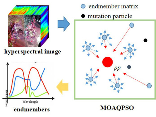
3.2. The MOAQPSO Algorithm for Endmember Extraction

MOAQPSO also uses particles to search the feasible solution space of the optimization problem. We assume that the whole image pixel set is $R=\left\{{\mathit{r}}_1,...,{\mathit{r}}_j,...,{\mathit{r}}_n\right\}$, where ${\mathit{r}}_j={(r_{1j},...,r_{ij},...,r_{Lj})}^{\mathrm{T}}$, n is the number of pixels, and L is the number of bands. The feasible solution space of the endmember extraction at time t can be defined as

$$X_i\left(t\right)=\left(e_{i,1}\left(t\right),e_{i,2}\left(t\right),...,e_{i,D}\left(t\right)\right)i=1,2,...,M$$

(26)

where $e_{ij}\in R$, $e_{ij}$ represents the jth endmember vector in the ith particle, M is the number of particles, and D is the number of endmembers.

Although there are no velocity vectors in MOAQPSO, $P_i\left(t\right)=\left(P_{i,1}\left(t\right),P_{i,2}\left(t\right),...,P_{i,D}\left(t\right)\right)$ is the best position of particle i, and $G\left(t\right)=\left(G_1\left(t\right),...,G_j\left(t\right),...,G_D\left(t\right)\right)$ is the best position of the entire swarm. The individual best position of each particle and the globally best position are updated in the same way as in PSO.

The position of the particle updates according to the following equation:

$$X_{i,j}(t+1)=p{d}_{i,j}(t)\pm \alpha \cdot \left|C_j\left(t\right)-X_{i,j}\left(t\right)\right|\cdot \ln \left[1/u_{i,j}(t)\right]u_{i,j}(t)\sim U(0,1)$$

(27)

where:

$$p{d}_{i,j}\left(t\right)={\phi }_j\left(t\right)\cdot P_{i,j}\left(t\right)+\left[1-{\phi }_j\left(t\right)\right]\cdot G_j\left(t\right){\phi }_j\left(t\right)\sim U\left(0,1\right)$$

(28)

$$C_j(t)=\frac{1}{M}{\displaystyle \sum _{i=1}^M{P}_i\left(t\right)}$$

(29)

Some research has proved that a linearly decreasing parameter $\alpha$ outperforms a constant, both in global search ability and local search ability [30]. Therefore, parameter $\alpha$ is linearly decreasing in this paper.

According to Definition (26), $e_{ij}\in R$. In order to meet the above conditions, the position of the particle should be adjusted after updating according to Equation (27). One strategy is finding the most similar pixel in set R with $X_{i,j}\left(t+1\right)$, calculated by Equation (27). The Euclidean distance and Spectral Angle Distance (SAD) are the commonly used criteria for similarity measure. As the Euclidean distance calculation has a lower computation complexity than that of SAD does, the Euclidean distance is used in this paper. It should be pointed out that any other strategy with the same function could replace the Euclidean distance.

Finally, the position of the particle updates according to the following equations as follows:

$${\tilde{X}}_{i,j}\left(t+1\right)={\mathit{r}}_b,b=\arg \underset{1\le k\le n}{\min }\left\{{\mathrm{distance}}_k\right\}$$

(30)

$${\mathrm{distance}}_k={\Vert {\mathit{r}}_k-X_{i,j}\left(t+1\right)\Vert }_2$$

(31)

where Equation (31) represents the distance between the jth endmember in the ith particle and the kth pixel.

With the increase in the number of iterations, the diversity of the population is reduced, and the algorithm can easily fall into a local optimum. Therefore, the algorithm would achieve a poor solution at a certain probability (pp), and this probability (pp) is called the mutation rate.

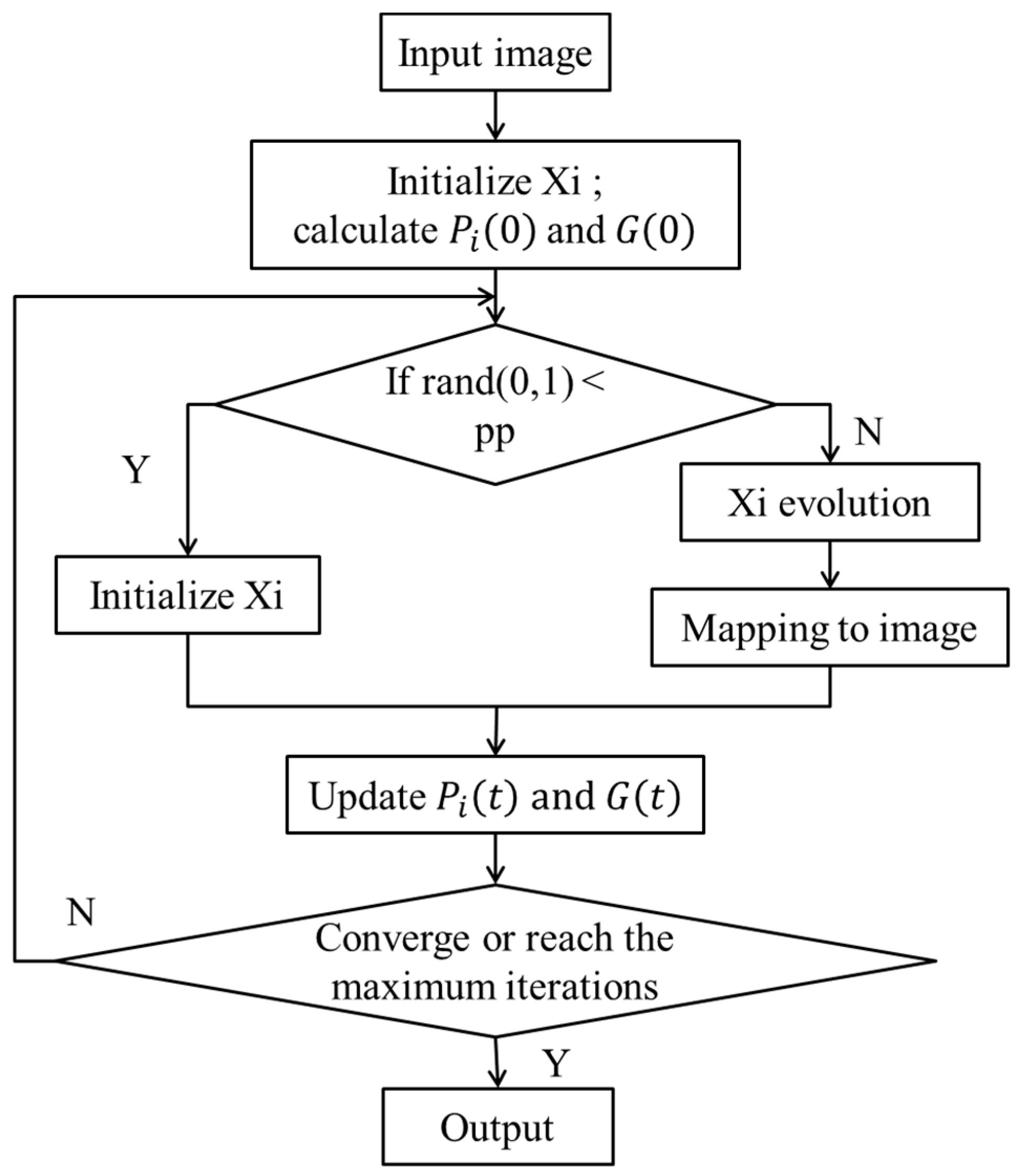
3.3. The Flow Chart of the MOAQPSO Algorithm

(1) Input Image

Due to the feasible solution space being defined as shown in Definition (26), the number of pixels in the input image has little impact on the search speed, which is different from the D-PSO. Therefore, a preprocessing for candidate endmember extraction is unnecessary.

(2) Initialization of the Population

At first, each individual $X_i$ in the population randomly selects D pixels from the image, as defined in Equation (25). Each vector $e_{ij}$ in each individual $X_i$ represents one pixel spectrum, which has a high dimension. In general, one particle is one possible endmember set.

(3) Calculating the Individual Best Position of Each Particle and the Global Optimum Position

Each particle, which is an endmember set, is applied with the simplex volume calculation using Equation (24).

$${\mathrm{fitness}}_i\left(t+1\right)=V\left(X_i\left(t+1\right)\right)$$

(32)

The individual best position of each particle is updated as follows:

$$P_i\left(t+1\right)=\{\begin{array}{cc}{X}_i\left(t+1\right)& \mathrm{if}V\left(X_i\left(t+1\right)\right)\ge V\left(P_i\left(t\right)\right)\\ P_i\left(t\right)& \mathrm{if}V\left(X_i\left(t+1\right)\right)\le V\left(P_i\left(t\right)\right)\end{array}$$

(33)

The globally best position is defined as

$$G\left(t+1\right)=\underset{P_i}{\arg \min }V\left(P_i\left(t+1\right)\right)$$

(34)

(4) Particle Evolution

Not all the particles evolve following the evolution Equation (27). Each particle is mutated with the mutation rate pp to obtain its associated mutated position by randomly selecting D pixels from the image. Otherwise, the position of the particle updates according to Equation (27), and the updated position should be mapped to the image according to Equation (30).

(5) Stopping Condition

If the result converges to a fixed value, or the iteration number reaches the maximum, the best endmember extraction solution is the output.

The flowchart of MOAQPSO is shown in Figure 1.

4. Experiments and Analysis

In this section, the extensive experiments conducted on one simulated and two real hyperspectral data are described. The algorithms used for comparison include N-FINDR, VCA, D-PSO and MOAQPSO. These typical algorithms are all based on the LMM and adopt the pure pixel assumption.

The SAD metric, which is widely used in the study of hyperspectral unmixing, was used to evaluate the endmember extraction results. The well-known SAD metric between pixel ${\mathit{x}}_a$ and ${\mathit{x}}_b$ is given by

$$\mathrm{SAD}({\mathit{x}}_a,{\mathit{x}}_b)={\cos }^{-1}\left(\frac{{\mathit{x}}_a\cdot {\mathit{x}}_b}{\Vert {\mathit{x}}_a\Vert \cdot \Vert {\mathit{x}}_b\Vert }\right)$$

(35)

where $\Vert {\mathit{x}}_a\Vert$ and $\Vert {\mathit{x}}_b\Vert$ are the norms of ${\mathit{x}}_a$ and ${\mathit{x}}_b$, respectively.

The RMSE was the other metric used to evaluate the results of the experiments. In the experiments on the synthetic data set, the abundance maps were available, therefore errors in the abundance maps could be calculated, and the RMSEs between the reference abundances and the calculated abundances were determined. In the experiments on the real data set, the RMSE between the original image and the reconstruction image was used because the abundance maps were not available.

N-FINDR, VCA, and D-PSO were selected for comparative purposes. In D-PSO, the random selection probability pp was set as 0.2, the number of particles was set to 10, and the VCA algorithm was used to obtain the 50 candidate endmembers, which could constitute a feasible solution space. In MOAQPSO, parameter $\alpha$ was linearly decreased from 1 to 0.5, according to previous studies [33]. The mutation rate was set to pp = 0.4 in the experiments, and the number of particles was set to 20 (synthetic data) and 30 (real data). The sensitivity of the parameter mutation rate pp was analyzed using the synthetic data.

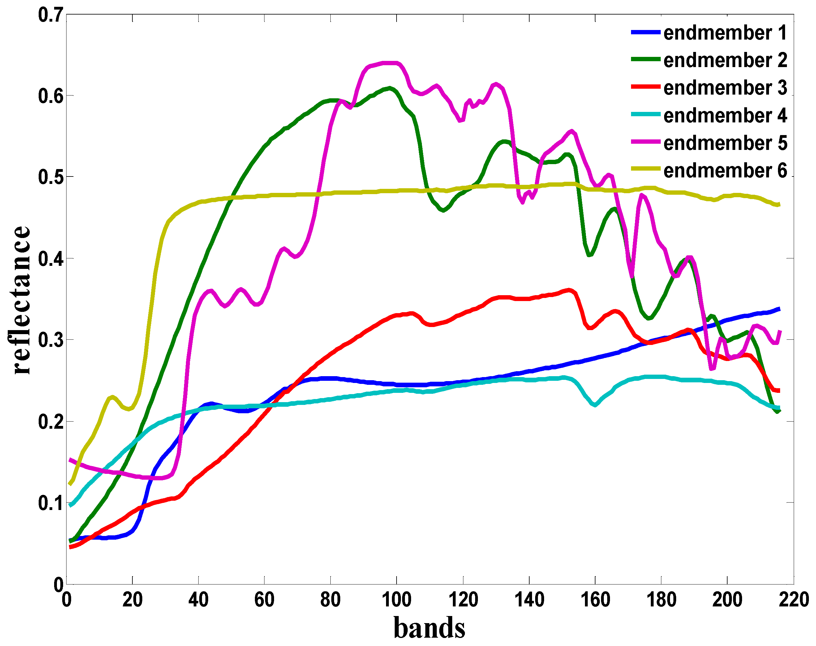
4.1. Synthetic Hyperspectral Image

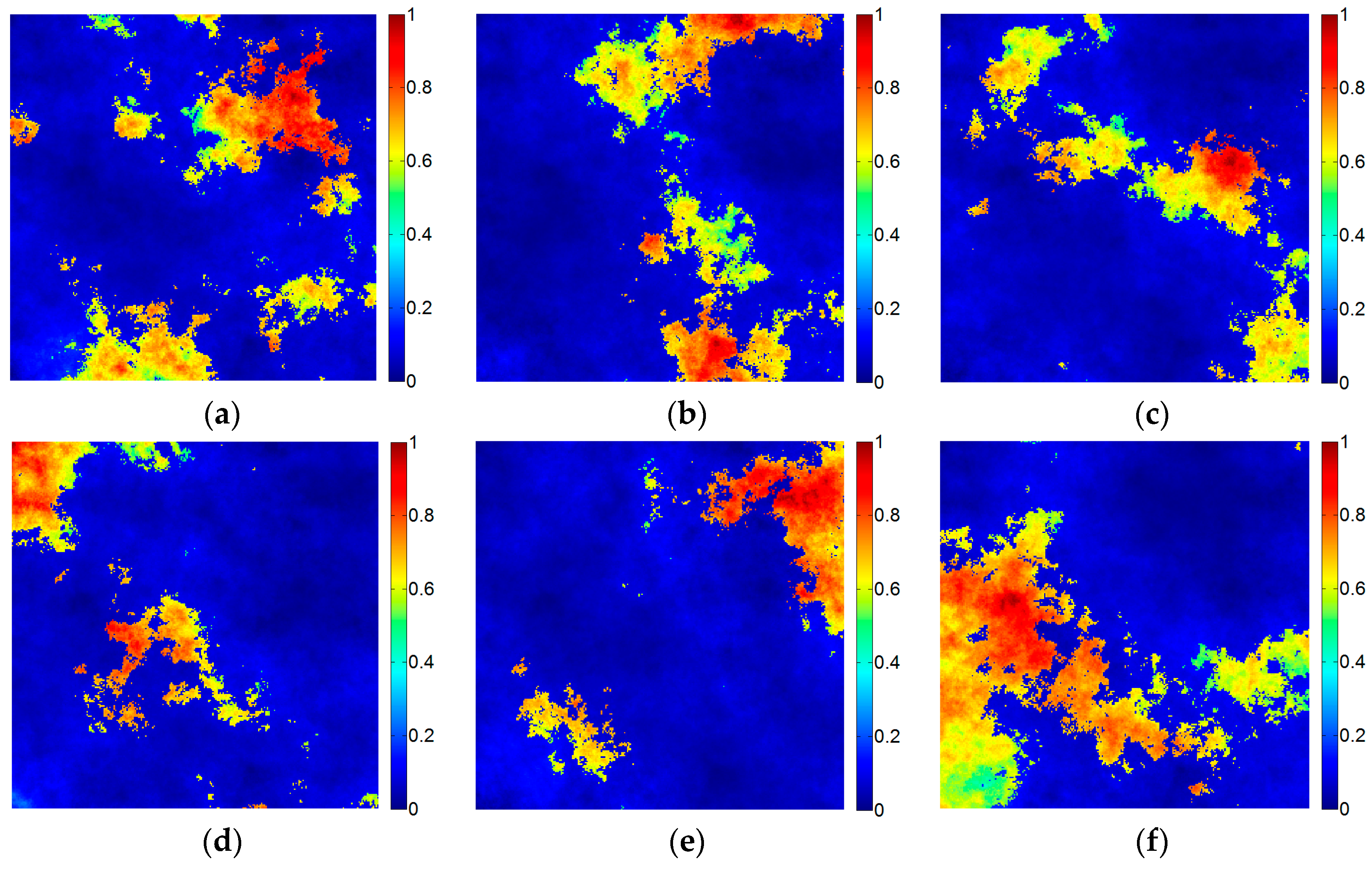
The simulated data cube was generated by six randomly selected spectral signatures (as shown in Figure 2). The simulated data contained 256 × 256 pixels covering 216 bands. The data was generated by the LMM. The fractional abundances satisfied the nonnegative constraint and the sum-to-one constraint. At last, the fractional abundances were piecewise smooth (i.e., they were smooth with sharp transitions), as shown in Figure 3. The simulated data were generated using the hyperspectral imagery synthesis toolbox for Matrix Laboratory (MATLAB) [34]. After the simulated data was generated, the scene was contaminated with Gaussian noise (SNR = 40 dB).

The quantitative evaluation metric for the endmember extraction results was the SAD value between each extracted endmember and the set of ground-truth spectral signatures. The lowest spectral angle represents the best performance.

Table 1. Comparison between the Spectral Angle Distance (SAD) values of N-FINDR, Vertex Component Analysis (VCA), Discrete Particle Swarm Optimization (D-PSO), and MOAQPSO.

SAD	N-FINDR	VCA	D-PSO	MOAQPSO
Endmember 1	0.04063	0.03624	0.06919	0.04063
Endmember 2	0.02331	0.02331	0.02355	0.02331
Endmember 3	0.04050	0.04050	0.04050	0.03624
Endmember 4	0.04555	0.04164	0.04189	0.04189
Endmember 5	0.02064	0.02064	0.02411	0.02064
Endmember 6	0.02331	0.02241	0.02279	0.02124
Mean	0.03232	0.03079	0.03701	0.03066

shows the SAD results obtained with N-FINDR, VCA, D-PSO, and MOAQPSO, respectively. The numbers in bold correspond to the best performances. From Table 1, we can see that the proposed MOAQPSO achieves a better result (a lower mean SAD) than VCA, N-FINDR, and D-PSO. D-PSO does not obtain a good result. The reason for this may be that the synthetic data used in the experiments only contain a small number of pure pixels, which have affected the results of the D-PSO algorithm.

Table 2. Comparison between the simplex volumes obtained by N-FINDR, VCA, D-PSO, and MOAQPSO.

	N-FINDR	VCA	D-PSO	MOAQPSO
Volume	0.0126	0.0133	0.0101	0.0135

shows the volume of the endmember set obtained with N-FINDR, VCA, D-PSO, and MOAQPSO, respectively. The numbers in bold correspond to the best performances. From Table 2, we can see that the proposed MOAQPSO achieved greater simplex volume than any other method. This is because the volume was the objective function of the proposed method.

Table 3. Comparison between the Root-Mean-Square Errors (RMSEs) of N-FINDR, VCA, D-PSO, and MOAQPSO.

	N-FINDR	VCA	D-PSO	MOAQPSO
Mean RMSE	0.2251	0.3174	0.3414	0.2957

shows a comparison of the mean RMSE between the reference and the abundance maps calculated by the endmember sets obtained by N-FINDR, VCA, D-PSO, and MOAQPSO, with the best results marked in bold. Although the mean RMSE of MOAQPSO is slightly higher than that of N-FINDR, it is still lower than that of VCA and D-PSO. This is because the objective function of MOAQPSO in the experiments was maximum-volume, and it achieved the greatest volume as shown in Table 2.

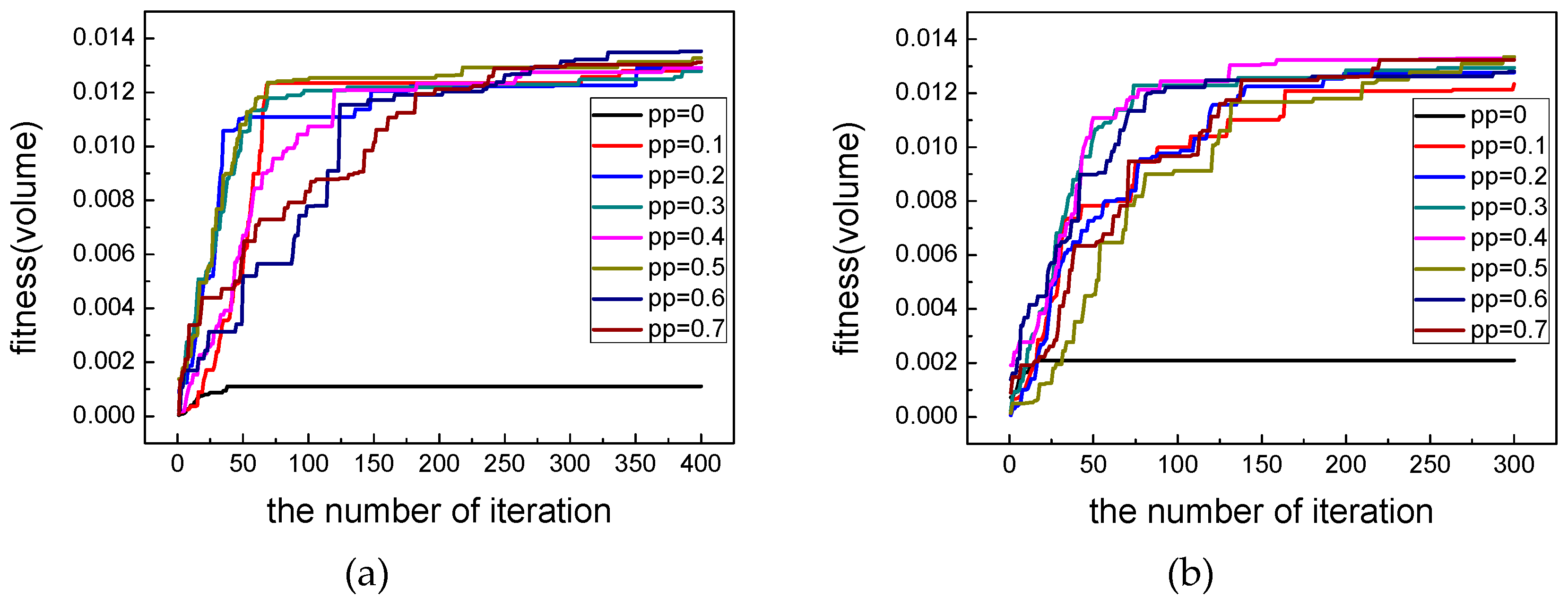
In this part, the sensitivity of the parameter mutation rate pp is analyzed. The population sizes were set to 20 and 30 respectively. The values of pp were set to 0, 0.1, 0.2, 0.3, 0.4, 0.5, 0.6, and 0.7, respectively. The experimental results are shown in Figure 4, where the horizontal axis represents the number of iterations, the vertical axis represents the volume, and the colors represent the pp value. From Figure 4, we can see that significant changes in the fitness function values occur over the first 150 iterations. After 200 iterations, the fitness function may increase slowly. A large population size reaches the optimal value with fewer iterations. This is because with a greater population size, the search scope increases, and a better solution is more likely to be found with fewer iterations. From Figure 4, we can also see that the effect of the mutation operation is obvious: MOAQPSO can obtain much better results with the mutation operation than without the mutation operation. However, the regularity is not so obvious: (1) all the mutation operations from 0.1 to 0.7 are clearly effective; and (2) a low mutation rate results in a fast convergence speed, and a high mutation rate results in a high precision.

4.2. AVIRIS Real Data Set

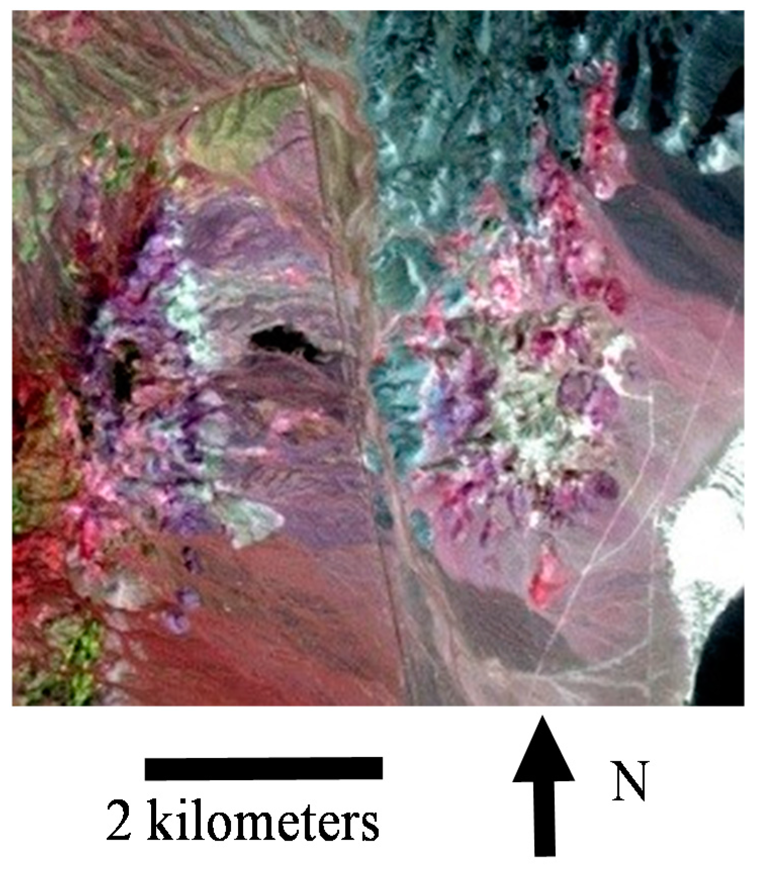
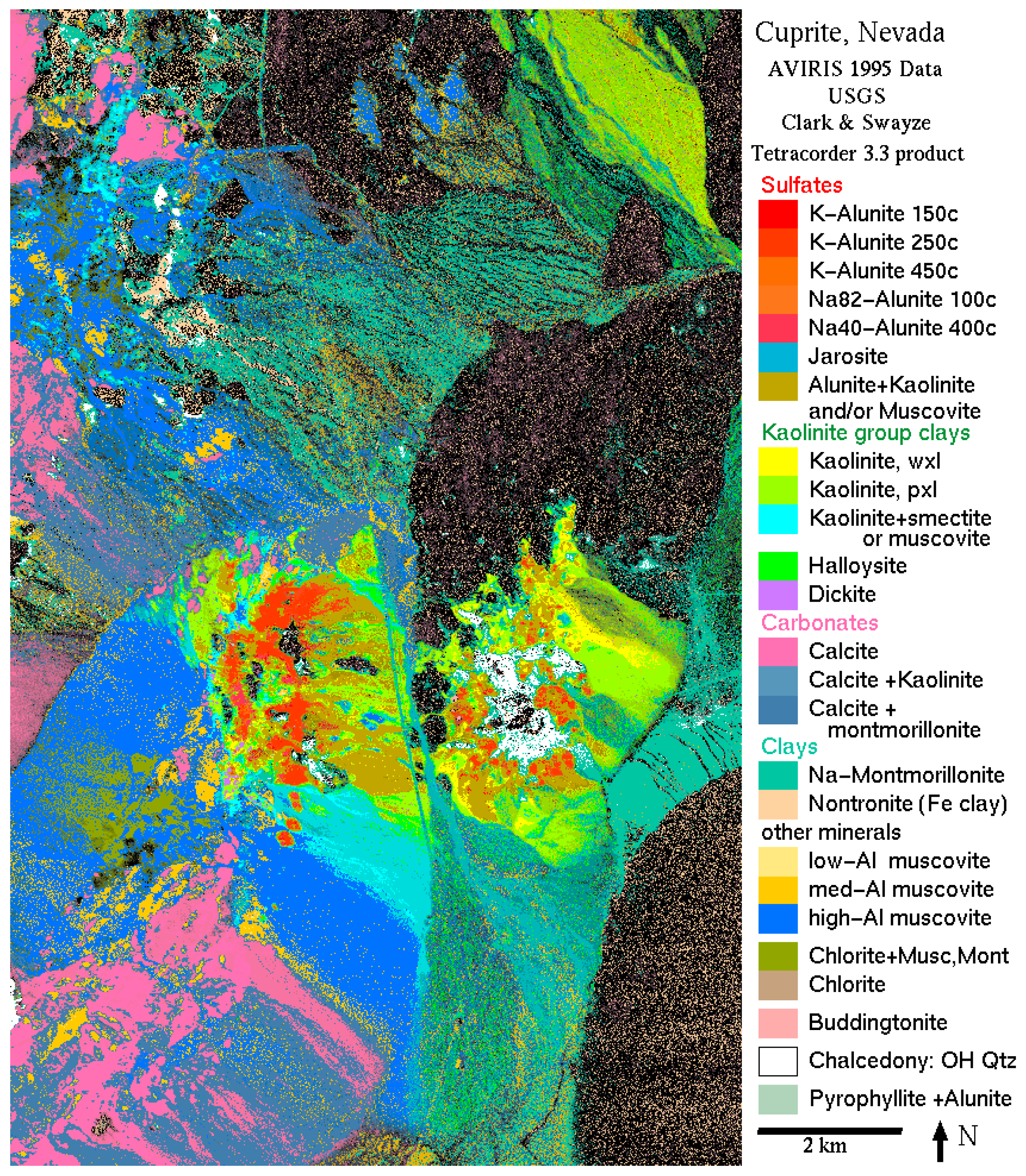
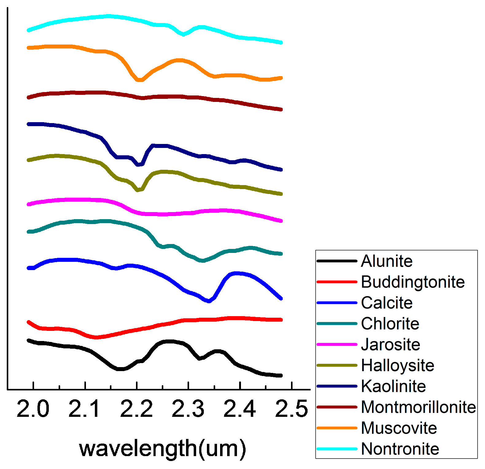
In this section, we perform MOAQPSO for endmember extraction from a real hyperspectral image. This real data set covering the Cuprite scene was captured by the Airborne Visible Infrared Imaging Spectrometer (AVIRIS) sensor in 1997, and a sub-scene is used in the experiments, which is shown in Figure 5. The size of the sub-scene is 350 × 400, covering the wavelength range of 2.0–2.48 μm. The data set has become a popular benchmark data set for algorithm evaluation, due to the extensive ground-truth data available for the scene from the United States Geological Survey (USGS). Swayze and Clark [35] have also produced a report about the ground truth of the area (shown in Figure 6).

It should be pointed out that: (1) The number of endmembers in this image is difficult to determine and the number of endmembers to be extracted was set to 10 for all the algorithms, according to Figure 6, and the reference spectra chosen from the USGS library are shown in Figure 7; (2) Due to the large number of pixels, which influences the speed of the mapping into image step in the MOAQPSO algorithm, another operation for acceleration is the selective mapping. In other words, mapping into image step does not work in each iteration. For example, if the length of the interval is set to 10, mapping into the image step will work once in every 10 iterations. In the real data experiments, the length of the interval was set to 10, and the number of iterations was set to 2000.

According to Figure 5 and Figure 6, the major minerals in the experiment region include Alunite, Buddingtonite, Calcite, Chlorite, Jarosite, Halloysite, Kaolinite, Montmorillonite, Muscovite, and Nontronite. The SADs were calculated between the reference spectra from the USGS library and the endmembers were extracted by those algorithms. The reference spectra chosen from the USGS library are shown in Figure 7. The performances of the algorithms were compared in terms of: (1) the number, type and average spectral angle of each mineral; (2) the volumes and RMSE of the endmember set. The results are shown in

Table 4. Comparison between the SAD values of N-FINDR, VCA, D-PSO, and MOAQPSO. * means that material cannot be extracted.

SAD	N-FINDR	VCA	D-PSO	MOAQPSO
Alunite	0.0555	0.0696	0.0513	0.0872
Buddingtonite	*	0.1601	*	*
Calcite	0.0761	0.0721	0.0685	0.0758
Jarosite	0.0652	0.0657	0.0652	0.0641
Halloysite	0.0680	*	0.1398	0.0752
Kaolinite	0.1558	0.1763	*	0.0858
Montmorillonite	0.1597	*	*	0.1597
Muscovite	0.0715	0.0819	0.0701	0.0670
Mean	0.0931	0.1043	0.0790	0.0878

,

Table 5. Comparison between the simplex volumes obtained by N-FINDR, VCA, D-PSO, and MOAQPSO.

	N-FINDR	VCA	D-PSO	MOAQPSO
Volume	9.1213 × 1014	6.1303 × 1014	1.9844 × 1012	9.2750 × 1014

and

Table 6. Comparison between the RMSEs of N-FINDR, VCA, D-PSO, and MOAQPSO.

	N-FINDR	VCA	D-PSO	MOAQPSO
Mean RMSE	2.9888	2.3058	2.8579	2.7931

.

Table 4 shows the SAD results obtained by N-FINDR, VCA, D-PSO, and MOAQPSO, respectively, with the best performance for each endmember marked in bold. From Table 4 we can observe that the endmembers extracted by the various algorithms were not the same. The proposed MOAQPSO and N-FINDR extracted seven different minerals, but failed to correctly extract Buddingtonite. VCA extracted six different minerals, but failed to correctly extract Halloysite and Montmorillonite. D-PSO extracted four different minerals, but failed to correctly extract Buddingtonite, Kaolinite and Montmorillonite. Although D-PSO achieved the minimum mean SAD, more classes’ spectra were ignored or repeated. Above all, the proposed MOAQPSO extracts a comprehensive endmember set with a higher precision than that of N-FINDR and VCA. Table 5 shows the volume of the endmember set obtained by N-FINDR, VCA, D-PSO, and MOAQPSO, respectively. The numbers in bold correspond to the best performances. Because the volume is computed by the objective function of the proposed method, the MOAQPSO algorithm achieves the maximum simplex volume, followed by N-FINDR, VCA, and D-PSO. Table 6 shows a comparison of the mean RMSE between the original image and the reconstruction image calculated by the endmember set obtained by N-FINDR, VCA, D-PSO, and MOAQPSO. The numbers in bold correspond to the best performances. Although the mean RMSE of MOAQPSO is slightly higher than that of VCA, it is lower than that of N-FINDR and D-PSO. This is because the objective function of MOAQPSO in the experiments is maximum-volume. If the objective function of MOAQPSO is the RMSE (named as MOAQPSO-2), the mean RMSE of MOAQPSO-2 is 2.1396. Compared with Table 6, we can see that the mean RMSE of MOAQPSO-2 is the lowest compared with that of N-FINDR, VCA, D-PSO, and MOAQPSO.

4.3. HYDICE Data Set

In this section, we perform MOAQPSO for endmember extraction from another real hyperspectral image. The hyperspectral data set, covering an area in a Washington DC Mall, was collected by the Hyperspectral Digital Imagery Collection Experiment (HYDICE) sensor. This image had 210 spectral channels ranging between 0.4 and 2.4 μm. Bands where the atmosphere was opaque or with a high noise level were omitted from the data set, leaving 180 bands. In this experiment, a subset of 80 × 130 was extracted from the original image. 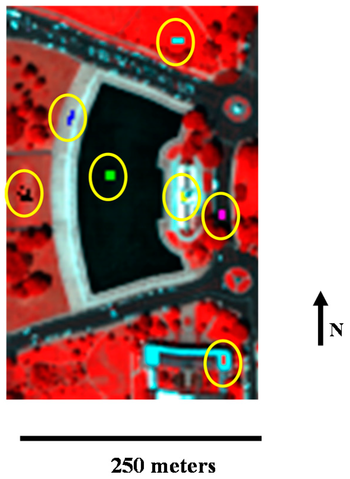Figure 8 shows the false-color image composed of bands 60, 27, and 17 for the red, green, and blue channels, respectively.

The sub-scene includes seven types of ground objects: water, tree, grass, roof 1, roof 2, street, and path. Seven kinds of pure pixels are selected manually, corresponding to the seven ground objects. In Figure 8, the areas in the yellow circles are the selected pure pixels. The averages of the selected pixels in each class were computed as the reference endmember signatures [36]. The SADs were calculated between the reference spectra manually selected from the image and the endmembers were extracted by the algorithms. The performances of the algorithms were compared in terms of: (1) the average spectral angle of each mineral; (2) the volumes and RMSE of the endmember set. The results are shown in

Table 7. Comparison between the SAD values of N-FINDR, VCA, D-PSO, and MOAQPSO.

SAD	N-FINDR	VCA	D-PSO	MOAQPSO
Roof 1	0.1746	0.1800	0.0071	0.0062
Roof 2	0.0386	0.0286	0.0258	0.0258
Water	0.1028	0.0908	0.1057	0.1028
Street	0.1810	0.1870	0.2130	0.2207
Path	0.0081	0.0181	0.0185	0.0052
Tree	0.0427	0.1176	0.0427	0.0366
Grass	0.0653	0.1012	0.0575	0.0653
Mean	0.0876	0.1033	0.0672	0.0661

,

Table 8. Comparison between the simplex volumes obtained by N-FINDR, VCA, D-PSO, and MOAQPSO.

	N-FINDR	VCA	D-PSO	MOAQPSO
Volume	1.3365 × 1022	7.1426 × 1021	8.6750 × 1020	9.8944 × 1021

and

Table 9. Comparison between the RMSEs of N-FINDR, VCA, D-PSO, and MOAQPSO.

	N-FINDR	VCA	D-PSO	MOAQPSO
Mean RMSE	63.237	35.572	43.130	45.037

.

As the number of pixels will influence the speed of mapping into image step in the MOAQPSO algorithm, another operation for acceleration is selectively mapping. The length of the interval was also set to 10 in this real data experiment as the first real image.

Table 7 shows the SAD results obtained with N-FINDR, VCA, D-PSO, and MOAQPSO, respectively, with the best performance marked in bold. From Table 7, we can see that all the methods extracted seven different materials and the proposed MOAQPSO achieves the minimum mean SAD value. Table 8 shows the volume of the endmember sets obtained with N-FINDR, VCA, D-PSO, and MOAQPSO, respectively. The numbers in bold correspond to the best performances. From Table 8, we can see that the MOAQPSO algorithm did not achieve a greater simplex volume than other methods, although the volume was computed as the objective function. The reason for this may be that there are many pure pixels in this data set, and it is very hard to get the optimal solution and the number of iterations is not enough in this case. Table 9 shows a comparison of the mean RMSE between the original image and the reconstructed image calculated by the endmember sets obtained with N-FINDR, VCA, D-PSO, and MOAQPSO. The numbers in bold correspond to the best performances. Although the mean RMSE of MOAQPSO is slightly higher than that of VCA and D-PSO, it is lower than that of N-FINDR. If the objective function of MOAQPSO is the RMSE (named as MOAQPSO-2), the mean RMSE of MOAQPSO-2 is 31.392. Compared with Table 6, we can see that the mean RMSE of MOAQPSO-2 is the lowest compared with that of N-FINDR, VCA, D-PSO, and MOAQPSO.

5. Discussion

In this paper, a novel Mutation Operation Accelerated Quantum-Behaved Particle Swarm Optimization (MOAQPSO) algorithm is proposed for hyperspectral endmember extraction. In order to ensure the effectiveness of QPSO for endmember extraction, some strategies are used, including: (1) The mutation operation. The mutation operation, which gives up the current position at a certain probability, is used to effectively maintain the population diversity and accelerate convergence. The effect of the mutation operation is obvious from the experiments results; (2) In this paper, a high-dimensional particle definition is proposed, and it ensures that each particle contains a physical significance for the endmember extraction.

The endmember spectra extracted by the proposed MOAQPSO method fit well with the references. From above experiments, we can see that: (1) the proposed MOAQPSO method can extract a more complete endmembers set with a lower mean SAD than that of N-FINDR, VCA, and D-PSO; (2) the MOAQPSO algorithm with volume as the objective function can achieve the maximum simplex volume, followed by N-FINDR, VCA, and D-PSO, and the MOAQPSO-2 algorithm with RMSE as the objective function achieves the minimum mean RMSE. However, there are still some unresolved issues and research on the use of QPSO for endmember extraction is still in its infancy. First, the proposed approach assumes that the image contains pure pixels. It cannot obtain the desired extraction results for highly mixed data and data with considerable noise. Second, the volume of the simplex is chosen as the fitness function in this paper. The fitness function can be replaced by any appropriate objective function. In our future work, we will try different kinds of fitness functions for endmember searching and endmember generation.

6. Conclusions

In this paper, a novel Mutation Operator Accelerated Quantum-Behaved Particle Swarm Optimization (namely MOAQPSO) approach has been proposed. All the particles in MOAQPSO have a quantum behavior instead of the classical Newton’s laws of motion that are followed in classical PSO. This quantum motion ensures that the particles can appear in any positions at a certain probability. The proposed algorithm introduces QPSO to endmember extraction, and a mutation operation is used to increase the population diversity, which has a significant effect, as proved by the experimental results. What is more, only two parameters need to be adjusted: $\alpha$ and pp. The default value is linearly decreased from 1 to 0.5 and 0.4, respectively, and the recommended range for these parameters is [0.5–1.5] and [0.3–0.7], respectively. The proposed MOAQPSO algorithm was evaluated by both synthetic and real hyperspectral data sets. The experimental results indicated that the proposed method obtained better results than the algorithms of VCA, N-FINDR, and D-PSO, with a lower mean SAD accuracy.