1. Introduction
As a key parameter of the surface energy budget, land surface temperature (LST) is directly related to surface energy fluxes and to the latent heat flux (evapotranspiration) and water stress in particular [
1,
2]. The LST is crucial for estimating the net radiation driven by the surface longwave emission [
3] and for computing soil moisture [
4,
5]. Moreover, LST is an essential climate variable for understanding meteorological and hydrological processes in a changing climate [
6,
7,
8]. Thus, understanding and monitoring the dynamics of the LST is critical for modelling and predicting climate and environmental changes and for other applications such as agriculture, urban heat island and vegetation monitoring [
9,
10,
11,
12].
The Chinese Gaofen-5 (GF-5) satellite is expected to be launched in 2017. One of its missions is to collect land information at high spatial resolution from visible to thermal infrared (TIR) spectral range for performing disaster monitoring. The multiple spectral-imager (MSI) is a payload onboard this satellite and has a 40-m spatial resolution for TIR channels. Development of a suitable algorithm for retrieving LST from the GF-5 data is urgently needed.
Remote sensing is a more effective method to map LST at large temporal and spatial scales than traditional measurement. However, accurate determination of the LST from satellite data is a difficult task because it is necessary to correct the remote sensing measurements for atmospheric absorption and emission and for the effect of surface emissivity, the latter generally differing from unity and being channel dependent [
13]. Efforts have been devoted to estimating LST from satellite measurements [
14,
15,
16,
17,
18,
19]. A complete review of different LST retrieval methods can be found in the literature [
20].
The selection of the LST algorithm for GF-5 data is based on a literature review and the characteristics of the GF-5 satellite data. The single-window method requires high-quality atmospheric profile and is sensitive to uncertainties in the atmospheric corrections. Considering the simultaneous retrieval of the LST and the land surface emissivity (LSE), the temperature and emissivity separation (TES) method may be a candidate. However, significant errors in the LST and LSE for the surfaces with low spectral contrast emissivity (e.g., water, snow, vegetation) can be caused by the TES [
21,
22]. Since the GF-5 satellite observes the land almost at nadir, the dual-angle algorithm was discarded. Among the various methods proposed for LST determination, the quadratic split-window (SW) algorithm has received considerable attention because of its simplicity. It can be written as [
13,
15]:
where
Ts is the land surface temperature (LST),
Ti and
Tj are the at-sensor brightness temperatures for two TIR channels,
A and
B are coefficients and
C is a constant. To correct the emissivity effect, different parameterizations of
A,
B and
C can be found in the literature: (i) Constant
C was formulated as a function of the mean (ε = (ε
i + ε
j)/2) and difference (Δε = ε
i − ε
j) of the two channel LSEs, keeping the other coefficients independent of LSE as in sea surface temperature (SST) retrieval [
23]. (ii) To make Equation (1) applicable to more general atmospheric conditions, Sobrino and Raissouni proposed modifying constant
C as the linear combination of ε, Δε and atmospheric water vapour content (W) [
24]. (iii) Assuming Δε = 0, François and Ottlé presented different coefficients for different ε values [
25]. (iv) Sun and Pinker addressed the SW coefficients according to different surface types to account for LSE effect [
26]. It should be noted that the land surface is complex and that the LSE may be quite different from unity and depends on the channel [
27]. Considering the effect of the emissivity, the quadratic SW algorithm may not work well. As François and Ottlé noted in their work, when ε is greater than 0.95, good accuracy can be obtained using the quadratic method with the emissivity-dependent coefficients. That means, when ε is low, the quadratic relationship no longer performs well or is changed. Therefore, the quadratic method should be re-examined and improved, especially for low emissivity.
This study aims to improve the quadratic SW method and develop a LST algorithm for GF-5 data. The variation in the channel emissivity will be also considered, which was not checked in the study by François and Ottlé. The paper is organized as follows:
Section 2 describes the data used in this study. The algorithm development is documented in
Section 3.
Section 4 presents the results using the simulated data and the sensitivity of the developed algorithm to the uncertainties of the input parameters is also analysed in this Section. The operational application of the algorithm to the satellite data is given in
Section 5.
Section 6 discusses the developed algorithm. Finally,
Section 7 describes the conclusions.
3. Algorithm Development
Using Equation (1), the dependence of
Ts −
Ti on
Ti −
Tj was examined for each combination of ε and Δε. For this purpose, the TOA
T10.8 and
T11.95 for two GF-5/TIR channels were simulated.
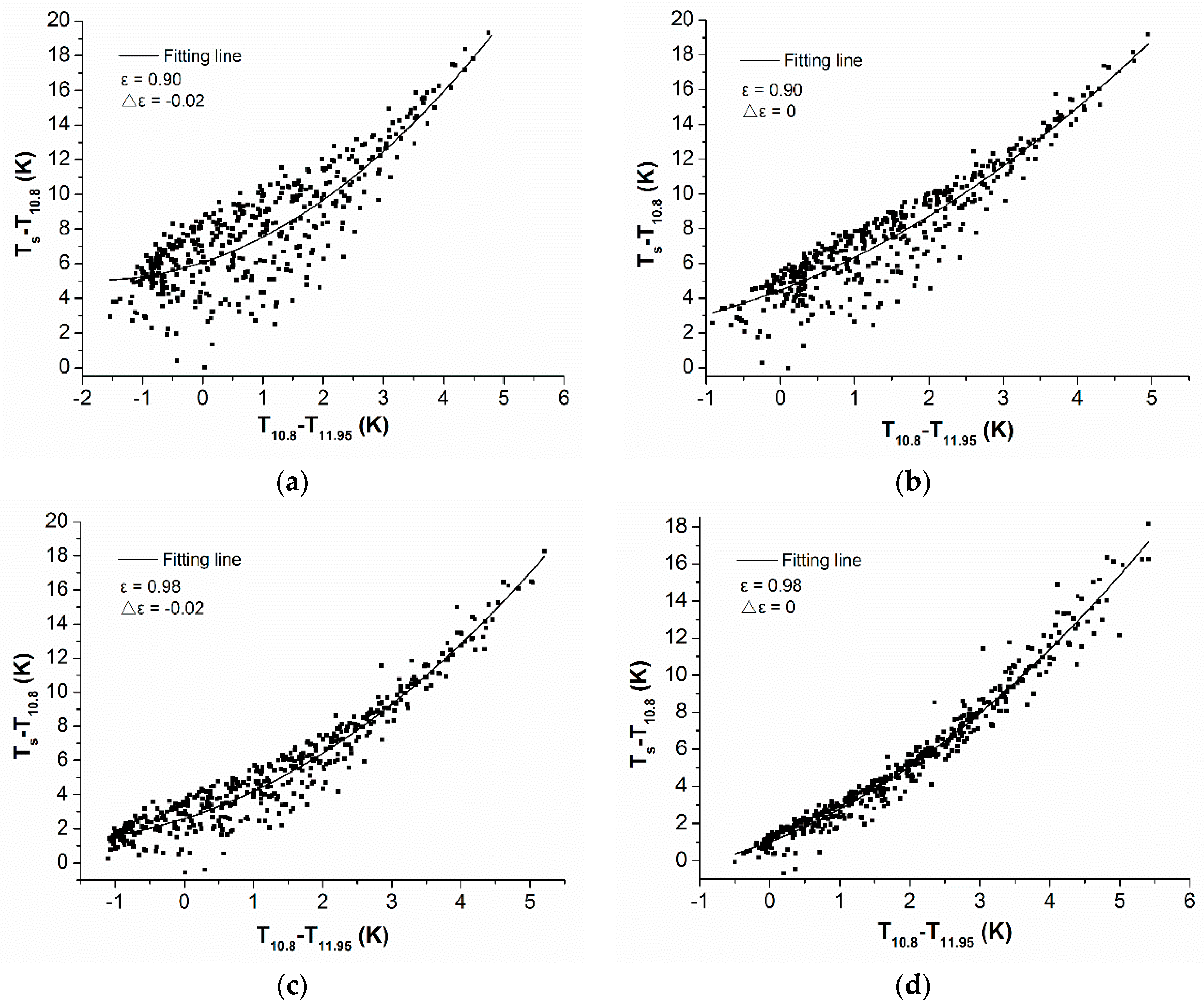
Figure 5 demonstrates that the variation in the emissivity deteriorates the quadratic relationship between
Ts −
Ti and
Ti −
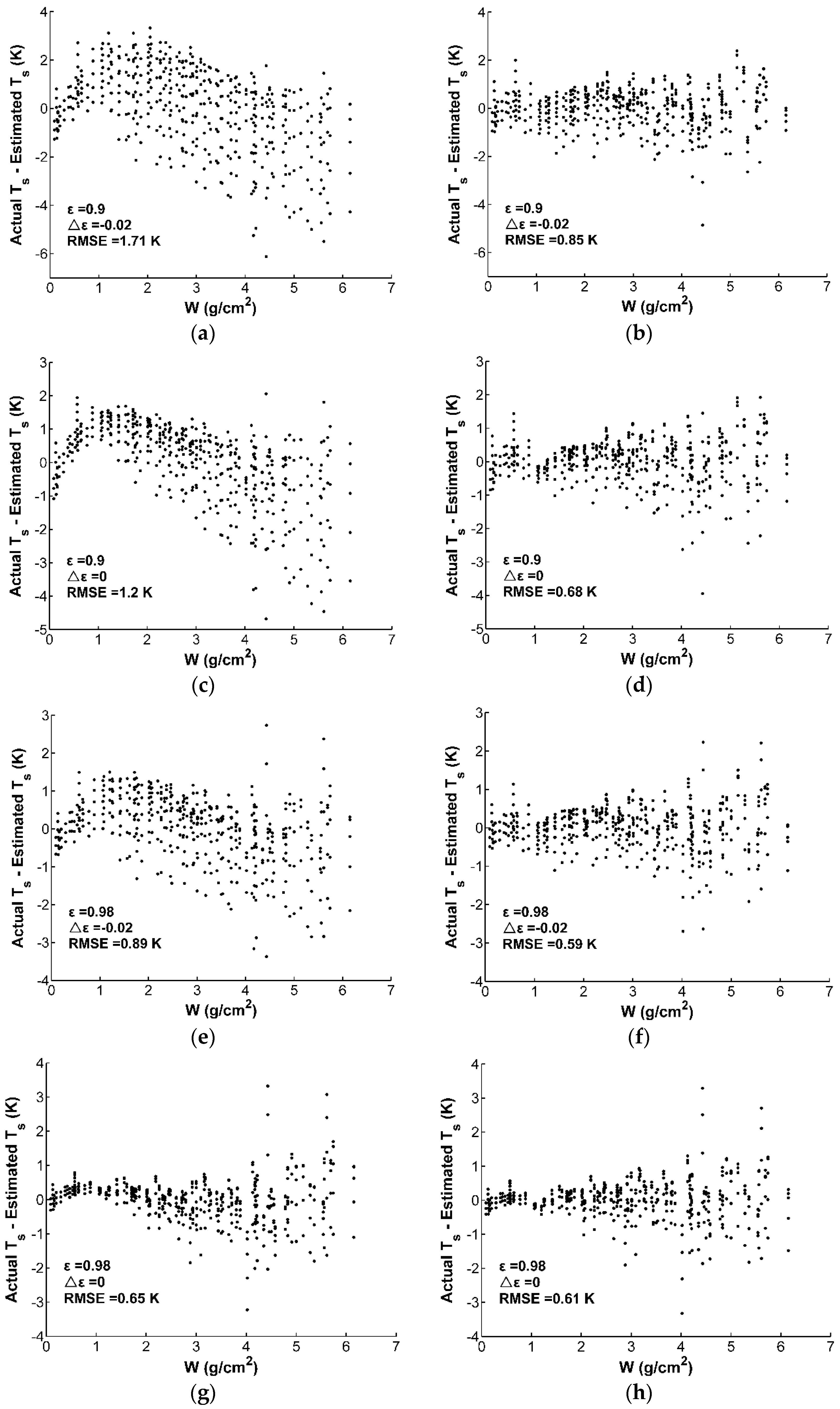
Tj, taking the combinations of (a) ε = 0.90 and Δε = −0.02, (b) ε = 0.90 and Δε = 0, (c) ε = 0.98 and Δε = −0.02 and (d) ε = 0.98 and Δε = 0 as examples.
Figure 5 confirms that Equation (1) works well for case (d). For smaller ε, the quadratic relationship is deteriorated for Δε of 0 and −0.02. Furthermore, Δε of −0.02 tends to intensify this deterioration. Therefore, Equation (1) would lead to large error for low emissivity, especially for the case of (a).
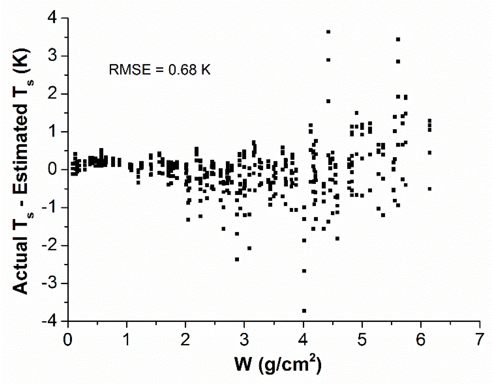
Assuming ε
10.8 = ε
11.95 = 1, Equation (1) yields
A = 0.2809,
B = 1.447 and
C = 0.17, with RMSE = 0.68 K.
Figure 6 is the plot of residual for the black body case, implying the applicability of Equation (1) for SST retrieval. For LST estimation, Coll [
15] has shown that the SW coefficients for SST can be used for LST retrieval if the emissivity effect is estimated. Therefore, we used the same
A and
B to develop the LST algorithm but modified
C to correct the emissivity effect.
Considering the worst performance of Equation (1) shown in
Figure 5a, constant
C in Equation (1) was investigated by maintaining coefficients
A and
B as 0.2809 and 1.447, respectively. It can be seen from
Figure 7 that constant
C displays a regular variation trend. For atmospheric profiles of W < 1 g/cm
2,
C ranges from approximately 5 K to 9 K and increases with W. To parameterize
C, the linear dependence on W can be used. For atmospheres of W > 1 g/cm
2, a larger range (approximately 0~9 K) was obtained, and the linear dependence on W appears to be unsatisfactory to parameterize
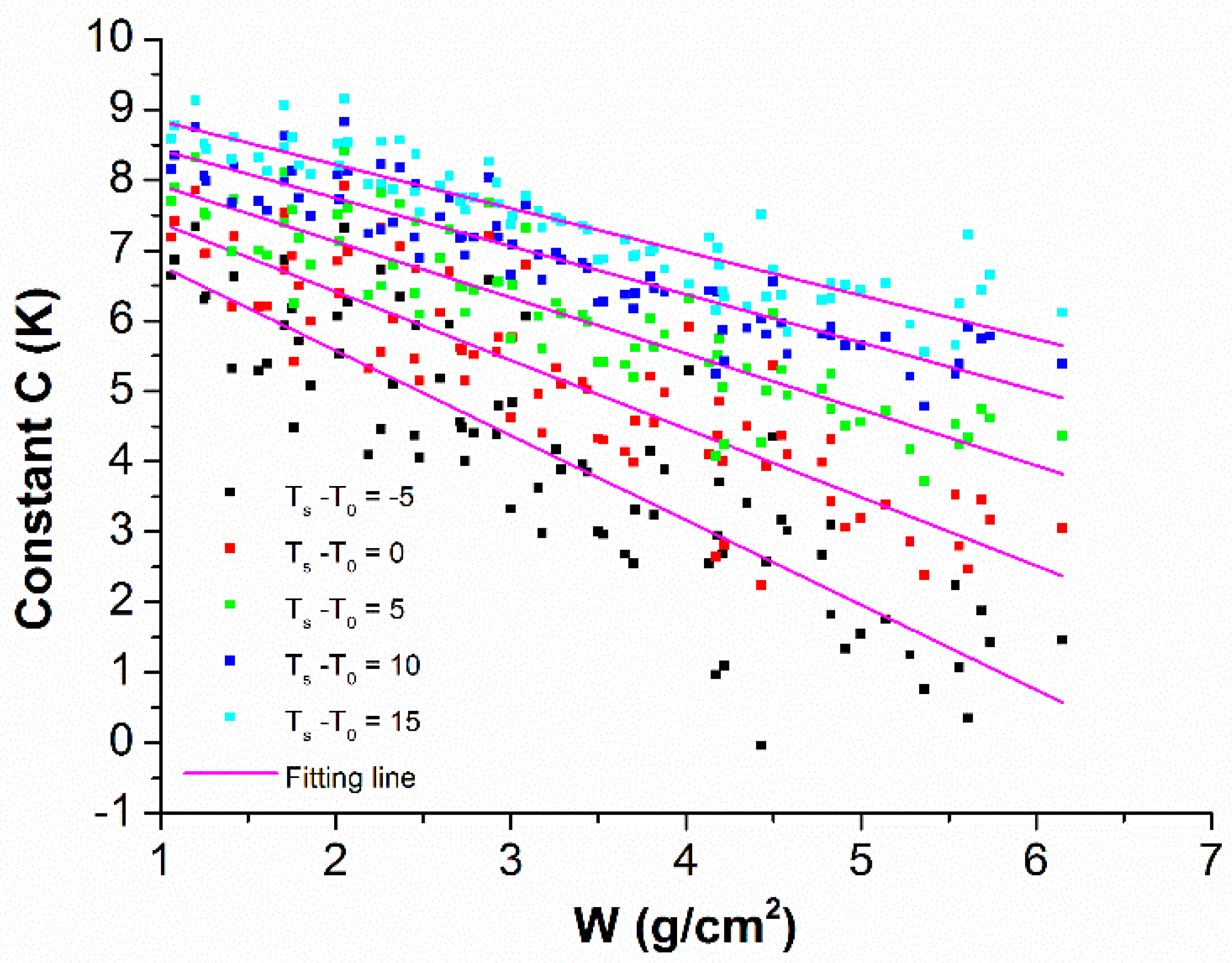
C. To explain the regularity of
C for W > 1 g/cm
2,
Figure 8 was produced. For a given surface-air temperature difference
Ts − T
0, constant
C displays a linear dependence on W. The slope and intercept of each linear relationship are listed in
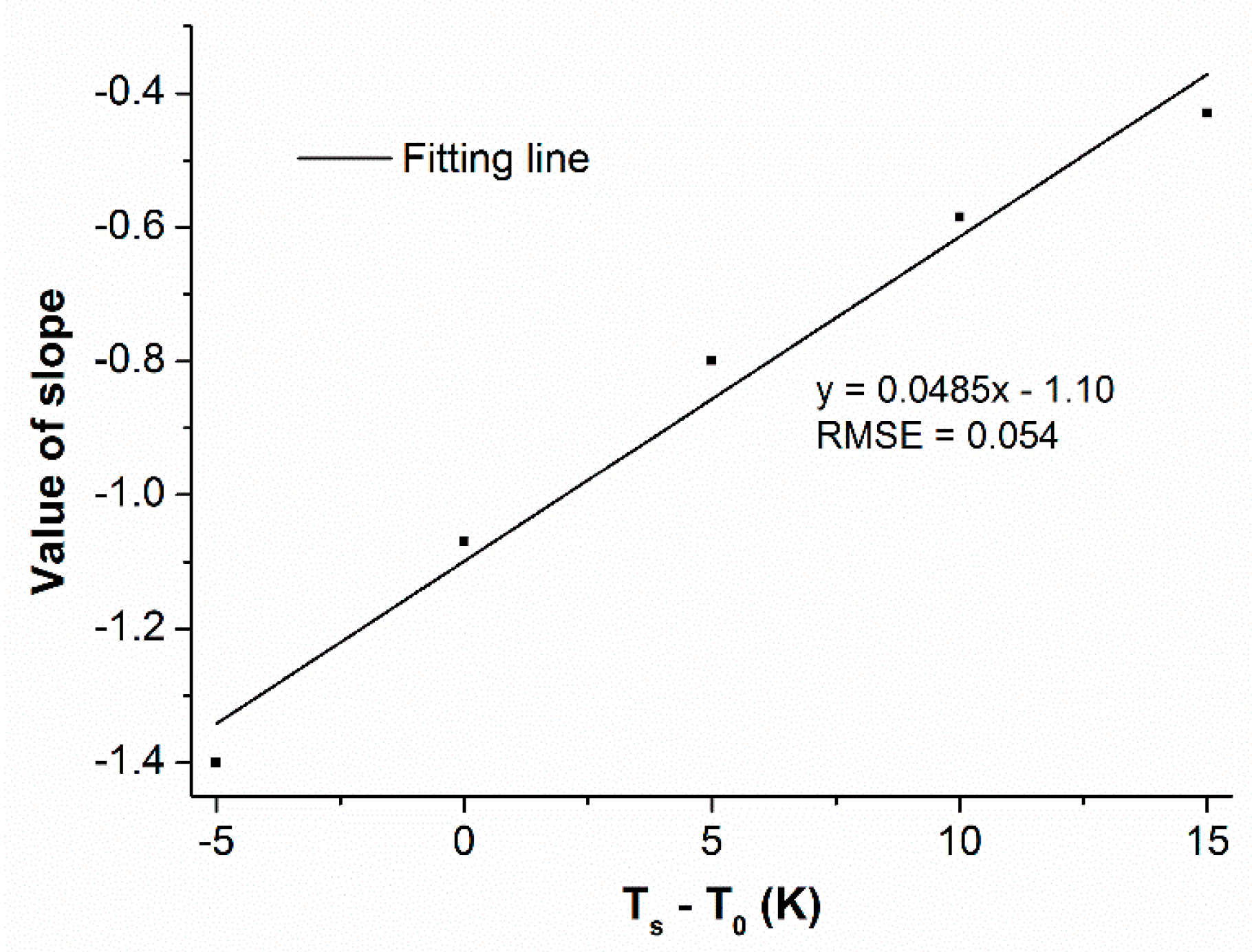
Table 1. As seen from
Table 1, although both the slope and intercept vary with
Ts − T
0, when the intercept is fixed using the mean of 8.73, the slope can be approximated by the linear function of
Ts − T
0, with a RMSE of 0.054 (
Figure 9). Based on these analyses, constant
C can be written as:
where
Cm = 2.63,
Cn = 5.56,
C11 = 0.0485,
C12 = −1.10 and
C2 = 8.73.
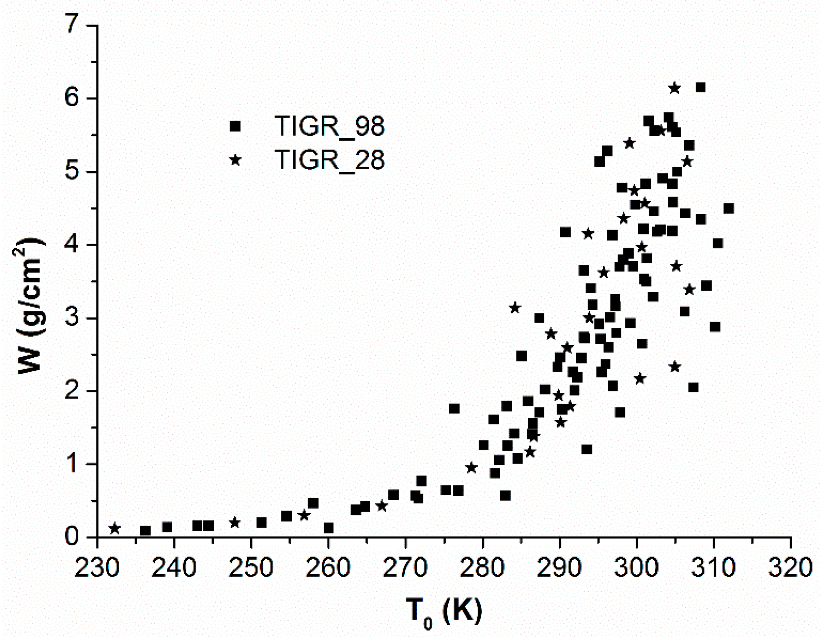
Because of the difficulties in obtaining atmospheric information, the parameter
T0 used in Equation (4) should be eliminated. According to the scatter plot between
W and
T0 in
Figure 2,
W can be approximated using an exponential function of
T0:
where α = 2 × 10
−7 and β = 0.0559. The fitting error on W is RMSE = 1.05 g/cm
2. Inverting Equation (5) yields:
Inserting Equation (6) into Equation (4) yields:
Because the terms
and
are both included in Equation (7), the dependence of
on
W was investigated as shown in
Figure 10, with a RMSE of 0.04 K. Therefore, Equation (7) can be expressed as:
where
Ca = −0.1357,
Cb = −0.958 +
= −15.441 and
Cc = 1.22 +
C2 = 9.95.
The residual of constant
C calculated by Equation (3) for W < 1 g/cm
2 and by Equation (8) for W > 1 g/cm
2 is shown in
Figure 11, with RMSE = 0.86 K.
Substituting constant
C into Equation (1) using Equations (3) and (8),
Ts can be estimated using Equations (9) and (10) for a given LSE:
To obtain stable retrieval accuracy for atmospheres with a
W of about 1 g/cm
2,
W was divided into two groups with an overlap of 0.4 g/cm
2, 0–1.2 and 0.8–6.5 g/cm
2, when the least-square fitting method was used to obtain the coefficients in Equations (9) and (10).
Table 2 lists coefficients
Cm and
Cn in Equation (9) and
C11,
Ca,
Cb, and
Cc in Equation (10) for the emissivity combinations presented in
Figure 5, with
A = 0.2809 and
B = 1.447. To compare the results, the coefficients and constant in Equation (1) for the same emissivity combinations are shown in
Table 3.
In Equations (9) and (10), the coefficients are dependent on the emissivity. Consistent with previous works [
23,
24,
30,
31], (1 − ε) and ∆ε were used to express coefficients
Cm,
Cn,
C11,
Ca,
Cb and
Cc because these six coefficients were generated based on the analysis of the emissivity effect on LST retrieval. Then, Equations (11) and (12) can be obtained:
Using the regression for the
W groups of 0–1.2 and 0.8–6.5 g/cm
2, the coefficients in Equations (11) and (12) were obtained and are shown in
Table 4.
6. Discussion
The quadratic expression in terms of
Ts −
Ti and
Ti −
Tj for LST retrieval received considerable attention due to its simplicity and the advantage of using the TOA brightness temperatures in two channels only. The quadratic method was proposed because the variation of the linear SW coefficient with the atmospheric situation can be approximately corrected by
Ti −
Tj [
15]. If W is disregarded, the quadratic SW method is a good choice for correcting the atmospheric effect for high emissivity but not for low emissivity.
For a given emissivity, the developed algorithm of Equations (9) and (10) that parameterized constant C in the quadratic SW method improves the LST retrieval accuracy, especially for low emissivity. Based on Equations (9) and (10), an algorithm with coefficients incorporating the emissivity, i.e., Equations (11) and (12) was developed. Parameterizing constant C led to the introduction of the atmospheric W into the LST retrieval algorithm. Despite the difficulty in determining W accurately, the sensitivity analysis of the uncertainty in W shows that if the error in W is 20%, the error in the LST estimation is still satisfactory, with a RMSE of 0.81 K. Notably, the main error of LST retrieval comes from instrument noise. Compared with Sobrino’s algorithm that uses W and was also developed based on the quadratic SW method, the algorithm presented in this study gives improved accuracy. A disadvantage of the presented algorithm is the different expressions for different W groups (0–1.2 g/cm2 and 0.8–6.5 g/cm2), which increases the complexity of the algorithm.
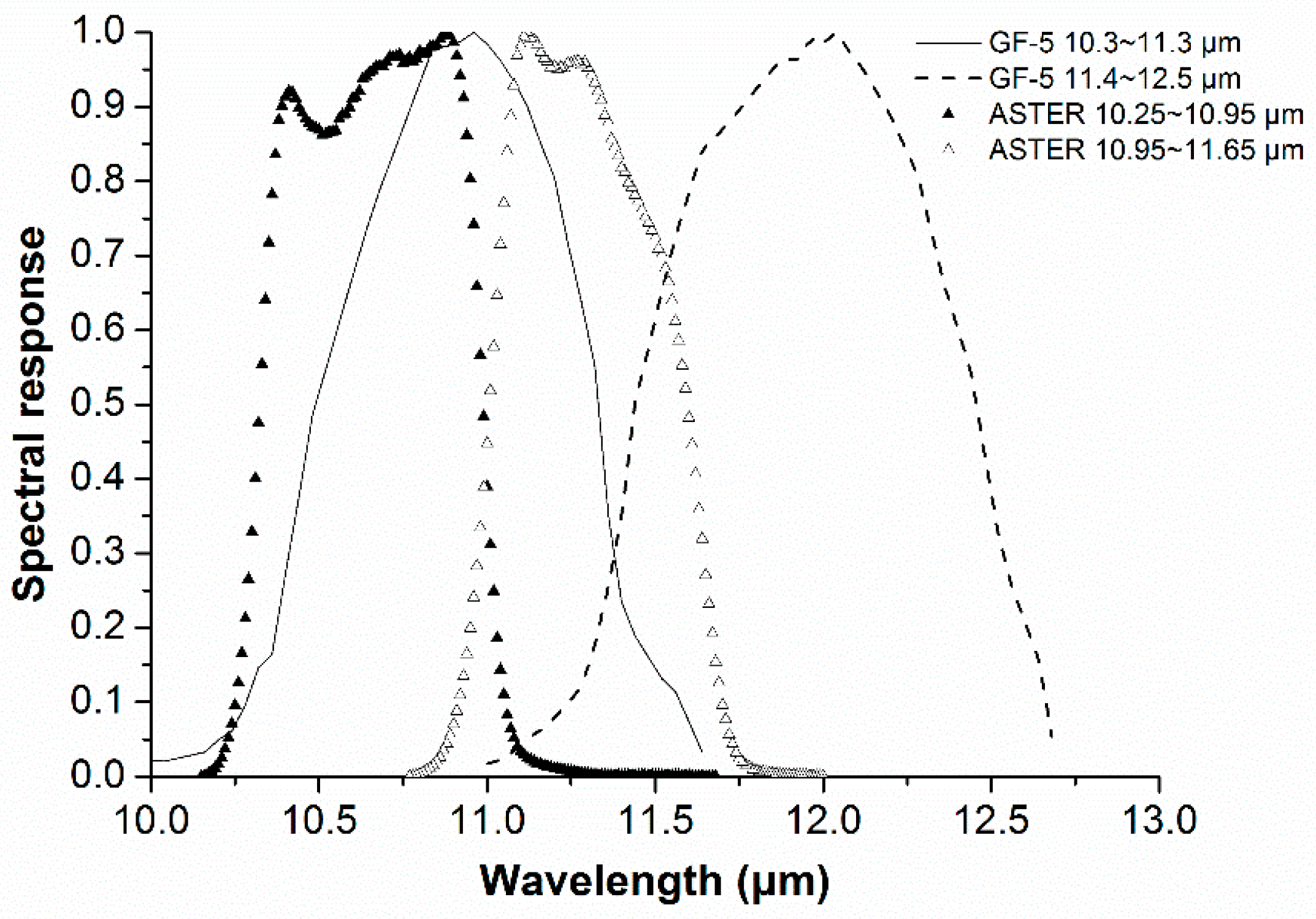
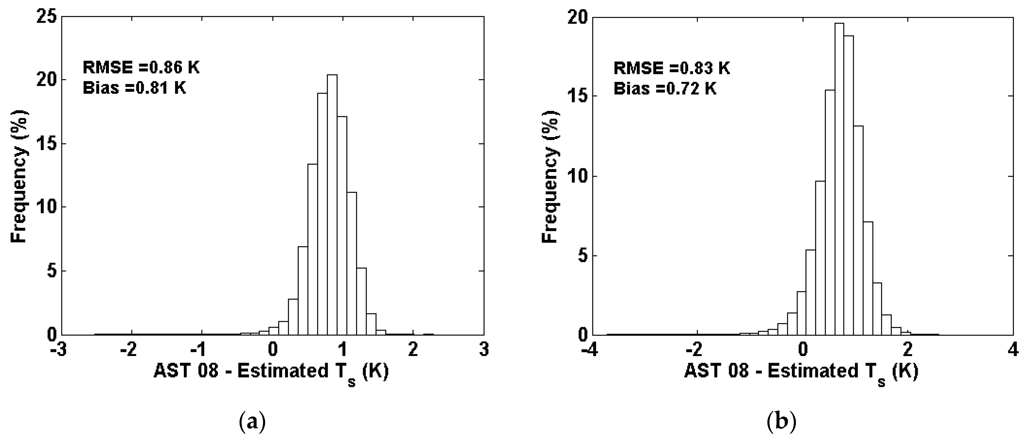
Using ASTER L1B data as a proxy to test the presented algorithm, the proposed algorithm underestimated LST by about 0.8 K, compared with AST 08 product. This difference may be related to the different atmospheric correct methods. AST 08 was generated using the TES algorithm, in which the accurate atmospheric correct is needed for each band. The proposed algorithm was based on the SW method, which uses different absorptions of two channels to eliminate the atmospheric effects. One may note that there is a difference between the spectral response functions of the SW channels for GF-5 and ASTER instruments, as shown in
Figure 1. The coefficients in Equations (11) and (12) given in
Table 4 and
Table 6 are therefore different for these two instruments, but the LST errors resulted from the algorithm itself are nearly the same (RMSE = 0.70 K for GF-5, RMSE = 0.69 K for ASTER) as shown in
Section 4.1 and
Section 5.2 if the appropriate coefficients are used in Equations (11) and (12). It should be also noticed that except for the brightness temperatures measured by the two SW channels, other input parameters (emissivities and W) have to be provided in Equations (11) and (12) to retrieve LST. For generating operationally LST product with GF-5 data, the emissivities and W in Equations (11) and (12) will be estimated from GF-5 data using the NDVI-based threshold method [
32] and the covariance-variance method [
33], respectively.
Notably, compared with other atmospheres with similar W, the atmospheric profiles with W = 4.02 g/cm
2, W = 4.43 g/cm
2 and W = 5.61 g/cm
2 lead to relatively large errors (approximately 3 K) in both Equations (1), (9) and (10), as shown in
Figure 13g,h. This may be related to the vertical distribution of water vapour in the atmosphere or the contribution of the other atmospheric constituents to LST retrieval. The details of this assumption can be analysed in future work.
7. Conclusions
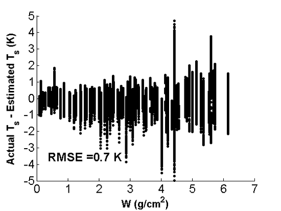
The quadratic relationship expressed by Ts − Ti = A (Ti − Tj)2 + B (Ti − Tj) + C works for high emissivities in both channels. When the emissivity becomes small, does such an equation perform well with satisfactory accuracy? This study first checked the performance of the quadratic SW method for different emissivities. Unfortunately, when the emissivity was low, the quadratic relationship between Ts − Ti and Ti − Tj deteriorated and thus led to a RMSE of up to 1.71 K. To solve this problem, the constant C was investigated for the emissivity combination of ε = 0.90 and ∆ε = −0.02, which gave the worst result in the quadratic SW equation. In this procedure, the coefficients A and B were set to 0.2809 and 1.447, obtained for a black body. Based on the observation that C was associated with W for W < 1 g/cm2 and with both T0 and W for W > 1 g/cm2, an equation that parameterized this constant was created. Following this approach, an operational algorithm, i.e., Equations (11) and (12) were proposed. This algorithm worked correctly on the simulations and yielded a RMSE of 0.70 K. The inter-comparison with AST 08 product showed that the proposed algorithm underestimated LST by about 0.8 K for both study areas when applied to ASTER L1B data.
Sensitivity analyses were performed for the instrument noise and the uncertainties in atmospheric W and LSE. Given NEΔT = 0.2 K, a 20% uncertainty in W and 1% uncertainties in (1 − ε) and ∆ε, the calculated result had a RMSE of 1.29 K. In contrast to the RMSE of 0.70 K related to the algorithm itself, the LST retrieval accuracy was changed by 0.59 K, 64.7% from the instrument noise, 19.1% from the uncertainty in LSE and 16.2% from the uncertainty in W.
The originality of this work lies in (i) the proposal of a different algorithm for LST retrieval and (ii) addressing the lack of an algorithm for the coming generation of GF-5 data.


