1. Introduction
Ocean swells are wind-generated surface gravity waves hardly affected by the local wind. They have a great impact on human activities such as port operations, sea-going, and coastal engineering and are crucial to many physical processes of the Earth system such as the energy and momentum fluxes at the air-sea boundary (e.g., [
1]). Swells are an important component of the wave climate, as they are prevalent in all basins of global oceans (e.g., [
2,
3]). Three main categories of data sources are usually involved in studies of swell climate: numerical model (e.g., [
3,
4]), voluntary observing ship (e.g., [
5]), and remote sensing (e.g., [
2,
6]). Each of them has its own advantages and disadvantages, with a related discussion found in [
4], but they are all powerful tools for the study of swell climate.
Regarding satellite remote sensing of swells, two types of sensors are used: altimeters and synthetic aperture radar (SAR). Spaceborne radar altimeters have been proved to be not only useful for studies of global wave climate (e.g., [
7]) but also studies of swell climate [
2,
8]. However, altimeters cannot distinguish different wave systems, which limits their applications on swell studies. SAR, on the other hand, can provide directional wave spectra using a special imaging mode termed “wave mode” [
9]. Due to the nonlinear process of wind-sea imaging [
10], it will be a hard task for SAR to measure wind-sea independently [
11]. Meanwhile, SAR is believed to be able to retrieve swell spectra and perform relatively well using quasi-linear inversion [
12], which makes it a useful tool for studying swells (e.g., [
13,
14,
15]). Regarding the swell climate, a global view of crossing swell is presented in [
6] using Envisat Advanced SAR (ASAR) data.
Numerical wave models are a helpful complement to observational data, providing new insights into global wave climate (e.g., [
3,
4,
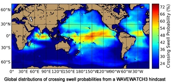
16]). Considering that the propagation of swells is understood from first principles, models are powerful tools for investigating swell propagation over global oceans. A global view of crossing swells as presented in [
6] using ASAR is easily available from a model hindcast. In this study, global distributions of crossing swells are presented using the WAVEWATCH-III
® (WW3) [
17] hindcast. However, the distinctions of these patterns and those from ASAR data lead us to a new question: Are the contemporary SAR data products from quasi-linear inversion suitable for such swell climate studies? Problems of SAR quasi-linear-inversion data that limit their application to swell climate are discussed, showing that special care is needed when using SAR wave data.
3. Results
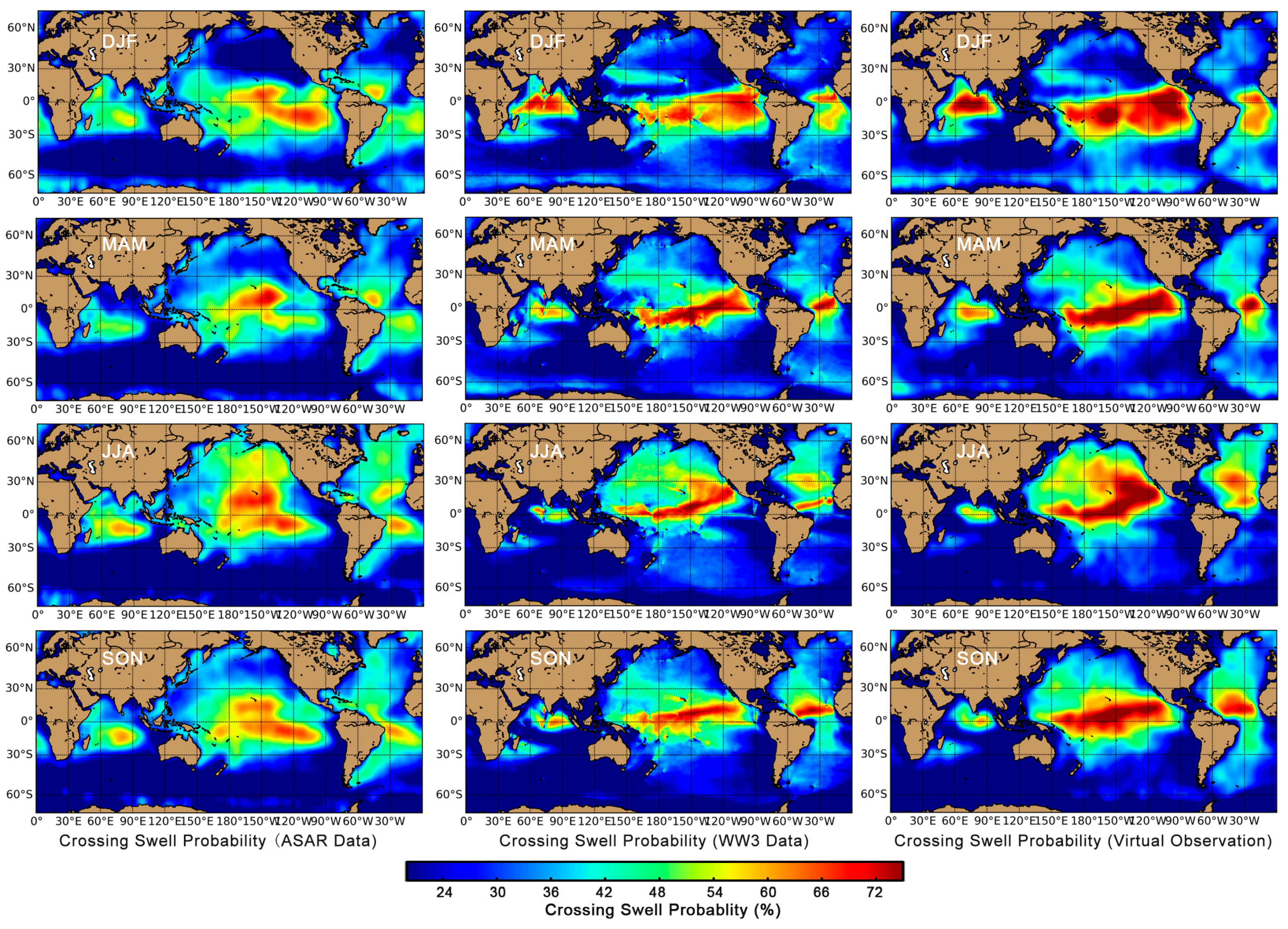
The global distributions of crossing swell probabilities from ASAR and from WW3 data are shown correspondingly in the left and middle columns of
Figure 1. The results from ASAR are almost identical with those of [
6], as the criteria are similar, while those from WW3 seem not to be reported elsewhere. Both the distributions from ASAR and WW3 show that crossing swells are likely to occur at low latitudes, and all ocean basins have some regions with high crossing swell probabilities which are referred to as “crossing swell pools” (CSPs) by [
6]. However, the spatial distributions of crossing swell probability derived from WW3 are, in fact, very different from those from ASAR data in any basin or season.
The distributions of crossing swell probabilities from ASAR have been described in [
6]. In the Pacific Ocean, although both the CSPs in WW3 and in ASAR data are located in the equatorial area, their shapes are different. The Pacific CSP in WW3 data is a zonal region across the basin connecting the north of New Zealand to Central America. This CSP in WW3 data is stable all over the seasons, with slight moving southward in DJF and northward in JJA, which means that crossing swells are more likely to occur in tropical regions of the summer hemisphere. In the Atlantic Ocean, the North and South Atlantic CSPs defined in ASAR data are not well-defined in WW3 data, while a small CSP in WW3 data is found almost in between the two CSPs in ASAR in all seasons, which means the distributions are opposite for WW3 and ASAR in the tropic Atlantic to some degree. This permanent Atlantic CSP in WW3 moves southward in DJF and northward in JJA in a range of around 10° latitudes. Besides that, two seasonal CSPs centered at around 20° S in DJF and 30° N in JJA are observed in the WW3 data, validating that crossing swells are more common in the summer hemisphere. Both the permanent CSPs of the Pacific and Atlantic in WW3 are in accordance with the “swell fronts,” where the swells from respective hemispheres have equal energy [
4,
24]. Considering the definition of crossing swell here, this consistency shows that the result from WW3 should be valid. In the Indian Ocean, the CSP in ASAR data located between 5° S and 20° S corresponds to a region with low crossing swell probability in WW3 data. Meanwhile, the Indian CSP in WW3 is traversed by the Equator in all seasons, and its size is the largest in DJF and smallest in JJA. In addition, the crossing swell probabilities in the Southern Ocean are relatively low in both datasets, but the values are higher in WW3 than in ASAR data, especially in the Pacific section.
4. Discussion
These differences between the results of WW3 and ASAR were not expected, as both of them are validated against in situ observations [
22,
25]. One possible conjecture of explaining the difference between the ASAR and WW3 results is that the spatial-temporal sampling of ASAR is not very homogeneous, as ASAR does not always work in wave mode and it can only inverse good-quality swell spectra in a certain range of wind speeds [
13]. To verify this conjecture, the WW3 data are collocated with ASAR as “virtual observations” of WW3 outputs using the same spatial-temporal sampling rate of ASAR. The corresponding results are shown in the right columns of
Figure 1. The coarser grids and less sampling in each grid did have some impact on the resulting global crossing swell probabilities, but the impacts are only on some details, while the general patterns almost stay the same. Therefore, the spatial-temporal sampling of ASAR is not the reason for this difference. Meanwhile, the result of virtual observation also shows that the spatial sampling of SAR is sufficient for wave climate provided that the data is of high quality.
Many studies of wave climate have been conducted using numerical models (e.g., [
4,
16]). Although numerical models produce unrealistic outputs under some certain conditions, the results of most model studies are consistent regarding climatology and seasonal variation. The comparison of wave climatology in Hawaii, where crossing swells are common, between model outputs and buoy measurements also shows good agreement implying that numerical models can reproduce crossing swells [
22]. Meanwhile, few wave climate studies used ASAR data of quasi-linear inversion until now. Although [
6] provides reasonable explanations for the results from ASAR in
Figure 1, these qualitative explanations are also applicable to our WW3 results. Therefore, we tend to believe there might be some problem with the way ASAR data are used.
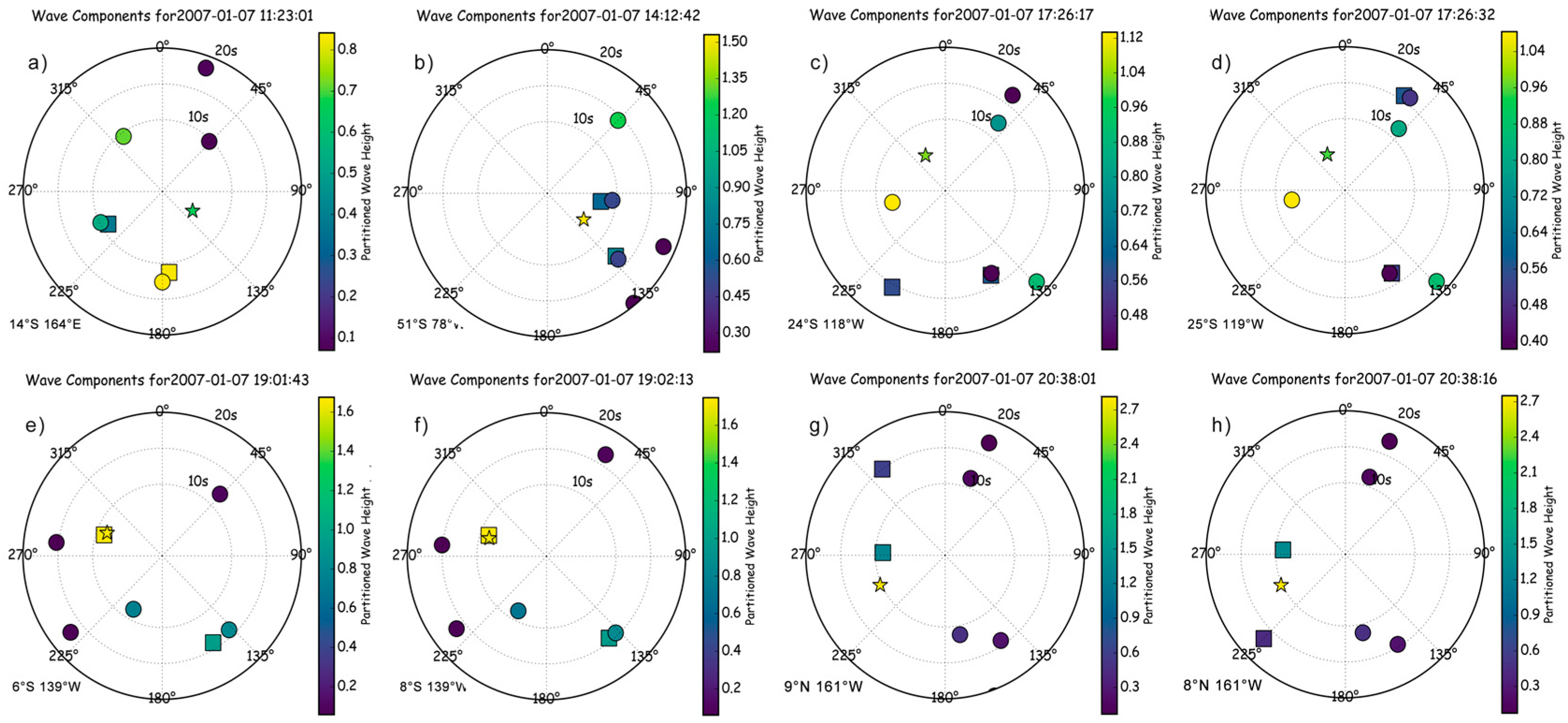
Examples of WW3 not in line with ASAR are shown in
Figure 2 using the WW3–ASAR collocated dataset. In
Figure 2a,b, each swell system inversed by ASAR can find a corresponding swell system in WW3. However, their orders regarding the wave height are not consistent in ASAR and WW3. In
Figure 2a, the 1st swell system in ASAR has good agreement with that from WW3, but the 2nd swell system in ASAR corresponds to the 3rd swell system from WW3 instead of the 2nd one, and the 2nd swell system is missed by ASAR. Similar conditions happen in
Figure 2b, where the 1st swell system is missed by ASAR. We have known that the quasi-linear inversion does not perform well in terms of retrieving wind-sea information, which limits its application on wave climate combining wind-seas and swells. However, even with the relatively improved performance on swells, the above effect of missing the 1st or the 2nd swells will still have some influences on SAR’s application on swell climate. In this case, both of the swell partitions inversed by SAR themselves are of high quality, but the entire ASAR record should not be regarded as high-quality. It is noted that the validation of ASAR [
25] is performed by comparing swell partitions so that the above problem of a missing component will not be revealed in the validation. Besides this missing of swell components, the so-called 180° ambiguity does not seem to be completely eliminated.
Figure 2c,d is from two successive ASAR records. In both of them, the first three components of WW3 are missed by ASAR, while ASAR swells have good agreement with the 4th and 5th WW3 swells in
Figure 2d. The northeastward swell from ASAR in
Figure 2d is in the southwest direction in
Figure 2c so that one of them must be wrong. In addition, although SAR quasi-linear inversion is believed to be unable to resolve the wind-sea,
Figure 2e,f is two successive records showing an example of wind-sea being well detected. The first swell component in ASAR is in excellent agreement with the wind-sea component in WW3. For some case studies, this condition might be good to show more possibilities of using SAR quasi-linear inversion in wind-sea. However, this unstable performance on wind-sea retrieving will also restrict SAR’s application on wave climate if all wave components resolved by the quasi-linear algorithm are regarded as swells.
Figure 2e,f is also two successive examples in which the ASAR are simply wrong in a wind-sea dominant case: the 1st swell in ASAR seems to match the wind-sea component in WW3, but with large errors in direction and energy, while the 2nd swell is not stably inversed and is not in line with any component in WW3.
Regarding the reasons of these errors, on the one hand, the performance of SAR is influenced by the angle between swell direction and antenna direction. Sometimes swells with a short wavelength can still be cut off in the azimuth direction, while other times the wind-sea with a similar wavelength can be retrieved in the range direction. It is noted that there is not a clear distinction between wind-seas and swells, especially for those at the transition state, which makes this issue more complex. On the other hand, due to other complex effects of SAR processing, such as non-linear imaging, not all swell components can be captured by the sensor even if they have more energy.
Another noteworthy point about these problems is that the validation of ASAR in [
25] is conducted using a “dynamic” scheme by which the refocusing and propagation of swells have already served as a quality control of ASAR data so that all the questionable partitions are filtered before comparison. However, these questionable partitions will still remain in the along-track ASAR data. Moreover, in the “dynamic” validation, the comparison between SAR-measured wave partitions and buoy-measured wave partitions is made without considering the energy order of swell components. Because of these potential problems, it would be helpful if a flag can be included in the Level 2 SAR quasi-linear product to indicate whether the first several partitions of the SAR are in accordance with the real sea state. Although it is hard to set this flag, as no reference for the sea state is available, this flag is important for many applications, especially with respect to the fact that new SAR missions such as Sential-1 might also deliver the same data products. A feasible way of doing it is to compare the SAR result with the model output, but this will cause other problems in the case where the model does not perform well.
In the case of Globwave data, all these four kinds of errors can be summarized as follows: the 1st and the 2nd swells retrieved by SAR is not correspondingly in line with the 1st and the 2nd swells in the model, and these errors are very common in ASAR data. To investigate the extent to which the SAR records would be impacted by such problems, the spectral distances between the 1st swell in the SAR data and the 1st swell in the WW3 data are calculated using the definition in [
21]:
where
f is the peak frequency,
θ is the peak direction, and the subscripts
m and
s indicate being from the model and from the SAR, respectively. The same calculation is conducted for the 2nd swells. If both the spectral distances of the 1st and the 2nd swells are less than 0.6 (in [
21], a threshold of 0.3 are employed, so that 0.6 should be a relatively loose threshold), the SAR record will be regarded as being in agreement with WW3. We find, surprisingly, that only 11,666 out of 2,201,782 (about 0.5%) SAR records without flags of bad or suspicious inversion agree well with the WW3. Although the model should not be regarded as the reference for observational data, this rate of agreement is still too low as a comparison. Therefore, these problems of SAR quasi-linear products will seriously influence the statistics, and these impacted SAR records should not be directly used in studies of swell climate, such as the global distributions of dominant swell heights and crossing swell probability, at least at this stage.
It has to be emphasized that this comparison is made on a “SAR-record level” instead of a “wave partition level.” For a SAR record that does not agree with the 1st and the 2nd swells in the model, it is completely possible that one or both of its swell partitions are valid. For example, in
Figure 2a,b, the SAR records do not agree with the WW3, but all the partitions of the SAR records can find their corresponding swells in WW3, which might be the 3rd or the 4th ones. Therefore, although these records are not suitable for wave climate studies, they can be useful in case studies of swells. Quality controls on each swell partition such as using swell refocusing (e.g., [
13]) can filter most of the badly inversed swell partitions and 180° ambiguity, and the problems shown in
Figure 2a,c will not have any impact on the case studies of swells. In fact, the SAR can obtain a good comparison with the WW3 on a “wave partition level” after the quality control and the right way of swell cross-assignment, which is detailed in [
26].
Therefore, the quasi-linear inversion can still provide large amounts of swell measurements of good quality. These data can be very useful in applications such as storm locating and swell tracking. Wave models especially do not perform well in many conditions, such as waves with strong currents or waves passing through small islands or atolls, while SAR can bring invaluable data to investigate and understand these phenomena. Despite its limitation on studying wave climate directly, SAR is a very powerful and irreplaceable tool for studying ocean waves, especially swells [
9].

 ,
, 