Pre-Launch JPSS-2 VIIRS Response versus Scan Angle Characterization

1
Science Systems and Applications, Inc., Lanham, MD 20706, USA
2
The Aerospace Corporation, El Segundo, CA 90245, USA
3
NASA Goddard Space Flight Center, Greenbelt, MD 20771, USA
*
Author to whom correspondence should be addressed.
Remote Sens. 2017, 9(12), 1300; https://doi.org/10.3390/rs9121300
Submission received: 31 October 2017
/
Revised: 4 December 2017
/
Accepted: 8 December 2017
/
Published: 12 December 2017
(This article belongs to the Collection Visible Infrared Imaging Radiometers and Applications)
Abstract
:On-orbit whisk-broom sensors have scanning mirror assemblies, whose reflectance variations with scan angle must be characterized prior to launch. One such instrument is the Visible Infrared Imaging Radiometer Suite (VIIRS) onboard the Joint Polar Satellite System 2 (JPSS-2) platform. The scanning optics inside VIIRS includes a four mirror rotating telescope assembly (RTA) and a half angle mirror (HAM), rotating at half the speed of the RTA, which de-rotates the light before it enters the aft-optics assembly. The angle of incidence (AOI) on the HAM varies with scan angle; all of the other optical components in VIIRS have a fixed AOI with scan angle. In general, the reflectance of the HAM will vary with AOI. This parameter is difficult to quantify once in orbit and therefore must be characterized pre-launch. Ground measurements were performed in the summer of 2016 to determine the relative reflectance change of the instrument with scan angle, referred to as the response versus scan angle (RVS). This work will describe the RVS testing performed and the results obtained, including an atmospheric water vapor correction and an uncertainty analysis. Results indicate that the reflectance variation with scan angle is small for spectral bands between 0.4 m and 4 m (less than 2% over the full range of AOI); in contrast, the reflectance variation is between 3% and 10% for the spectral bands in the 8 m to 12 m range. Uncertainties are below 0.05% in the reflective solar spectral region and below 0.26% in the thermal emissive spectral region. Comparisons to previous VIIRS builds (on the SNPP and JPSS-1 satellites) show comparable performance.
1. Introduction
Space-borne remote sensing instruments have been critical to the development of Earth science, including applications to land, ocean, and atmospheric science disciplines [1,2,3]; one such sensor is the Visible Infrared Imaging Radiometer Suite (VIIRS) that has flown on the Suomi National Polar-orbiting Partnership (SNPP) since 2011 [4,5] and is scheduled to launch on the Joint Polar Satellite System 1 (JPSS-1) platform in November 2017 [6]. The third sensor in the series, scheduled to launch aboard the Joint Polar Satellite System 2 (JPSS-2) platform in 2021, is currently undergoing ground testing at the sensor vendor test facility (Raytheon El Segundo). It is critical that certain parameters are characterized prior to launch, as they are difficult to update once the sensor is on orbit. This work focuses on the characterization of one of those parameters, the JPSS-2 VIIRS response versus scan angle (RVS), which measures the relative change in the reflectance of the optics with scan angle. Testing was performed in the summer of 2016 by the sensor vendor to measure the JPSS-2 VIIRS RVS.
The RVS was also characterized for the two preceding VIIRS sensors pre-launch [7,8]. The testing methodology has largely remained consistent between the three sensor builds. However, some of the analysis has been updated in this work including an atmospheric water vapor correction [9] and an improved uncertainty analysis. Additionally, some of the model assumptions will be reconsidered.
Section 2 will provide a brief overview of the VIIRS sensor as well as the RVS testing approach. The RVS analysis methodology is described in Section 3 including the atmospheric water vapor correction and uncertainty analysis. Section 4 will detail the results of the analysis and the comparison of JPSS-2 VIIRS to earlier VIIRS builds. Lastly, Section 5 will provide some conclusions.
2. Overview
2.1. VIIRS Overview
VIIRS is a cross-track scanning radiometer that was designed to fly aboard satellites in a polar, sun-synchronous orbit, giving it the capacity to image the Earth twice a day [4,7]. The VIIRS optical path from the entrance aperture first passes through the rotating telescope assembly (RTA), which is composed of an afocal three mirror anastigmat followed by a fold mirror [4,6]. The RTA rotates once about every 1.78 s perpendicular to the spacecraft’s direction of motion, viewing a ±56 degree swath through the Earth view port. Additionally, the RTA views three calibration targets to maintain the instrument calibration on orbit: a deep space view (SV) at about −65 degrees scan angle used as a dark reference; a view of the internal blackbody at about 100 degrees scan angle used for emissive band on-orbit calibration; and a view of the onboard solar diffuser (SD) at about 157 degrees scan angle, which provides a reflective band calibration target when illuminated by the Sun. The light exiting the RTA is directed onto a two-sided rotating fold mirror, referred to as the half angle mirror (HAM), that rotates at half the speed of the RTA, de-rotating the light beam and directing it into the fixed aft-optics. The optical path then passes through a fold mirror and a four mirror anastigmat as it enters the aft-optics. The visible and near infrared light is then reflected by a dichroic beamsplitter onto a focal plane array (FPA). Longer wavelengths are transmitted and then encounter a second dichroic beamsplitter that separates the short and mid-wave infrared (SMWIR) from the long-wave infrared (LWIR) and directs each to a separate FPA.
There are 21 spectral bands and one pan-chromatic band (referred to as the day–night band, or DNB) covering a wavelength range from 0.41 m to 12 m onboard VIIRS [6,7]. Nine visible and near infrared channels are located on the first FPA, whose temperature floats with the instrument; an adjacent temperature controlled FPA (tied to an intermediate stage of the passive cooler) contains the DNB. There are eight channels on the SMWIR FPA and four channels on the LWIR FPA; both of these FPAs are enclosed in dewars tied to the cold stage of the passive cooler, which will maintain their FPA temperatures on orbit at around 82 K.
The spectral bands are listed in Table 1 along with their center wavelengths. Bands are named beginning with ‘I’ for imaging resolution or ‘M’ for moderate resolution. The bands with center wavelengths below 3 m were designed to measure the sunlight reflected off the Earth (referred to as reflective bands) and the bands with center wavelengths above 3 m were meant to observe the radiance emitted by the Earth (referred to as emissive or thermal bands). Note that, although bands M16A and M16B are treated separately pre-launch, on orbit, they will be combined into one spectral band. Each band has 16 detectors (32 for the imaging bands), aligned parallel to the direction of motion, that image the Earth’s surface with footprints adjacent to each other.
On orbit, the calibration of both the reflective and emissive bands is maintained largely through views of the onboard calibration targets (solar diffuser and internal blackbody, respectively) [4,5]. To transfer the calibration from either target to the Earth view data, knowledge of the RVS is required. As a result, the RVS plays a critical role in the maintenance of the calibration for all bands on orbit. Moreover, this quantity is difficult to characterize on orbit with sufficient accuracy; therefore, the RVS of all 22 bands must be characterized prior to launch.
2.2. Testing Overview
The sensor vendor (Raytheon, El Segundo, CA, USA) performed testing in the summer of 2016 to characterize the RVS for all bands on JPSS-2 VIIRS. The test setup used to measure the JPSS-1 VIIRS RVS was described in detail in [8]; as the testing for JPSS-2 VIIRS RVS was very similar to the previous sensor build, only a brief description is included here.
The testing was performed under laboratory ambient conditions and the VIIRS instrument was placed on a rotating table with the scan plane perpendicular to gravity. This allowed the instrument to view external sources by either rotating the instrument (for the reflective bands) or moving the source to a different location (for the thermal bands) while keeping the illumination level constant.
An integrating sphere was used as a source for the reflective solar bands and the internal blackbody was used as a dark reference. Light from four 200 W lamps illuminated the sphere, whose exit aperture as viewed from VIIRS was an extended source. The instrument was rotated to view the integrating sphere at different scan angles and was operated successively at three different integration times per scan angle (to ensure that all reflective bands observed an unsaturated signal while viewing the same source configuration). The scan angles measured for JPSS-2 VIIRS are listed in Table 2 in the order measured (including repeated measurements at ∼−8 degrees used to assess source stability). Temperature and humidity monitors (THM) were placed near the exit aperture of the integrating sphere and near the VIIRS nadir door.
An external blackbody with a large area cavity, the internal blackbody, and an external dark reference target were used as sources for the thermal emissive bands (set to 345 K, 312 K, and ambient or 294 K, respectively). The external blackbody position was changed such that VIIRS viewed this blackbody at the scan angles listed in Table 2, in the order measured (measurements were repeated at ∼−8 degrees to assess source stability). The Earth view was rotated to start at ∼−70 degrees scan angle, allowing a full view of the external blackbody at the SV scan angle. The external reference target was placed at about 55.5 degrees scan angle.
3. Methodology
The RVS is modeled as a quadratic polynomial in HAM angle of incidence (AOI) [8], or
The final RVS is normalized to the RVS at the SV HAM AOI (AOI) of 60.47 degrees. The RVS at a specific AOI is denoted by a subscript; for instance, the RVS at AOI is written as RVS. The are free parameters used to fit the measured RVS to the measured AOI. The HAM AOI is related to the scan angle by the following [8]:
where the 28.6 degree angle accounts for the out-of-plane tilt of the HAM that folds the light into the aft-optics. The remainder describes the de-rotation of the light beam as it passes from the RTA through the HAM.
As VIIRS scanned across an external source (either the integrating sphere or the external blackbody), a scan profile was formed consisting of a plateau corresponding to scan angles where the VIIRS footprint was fully inside the source aperture and decreasing signal before and after the plateau corresponding to scan angles where the VIIRS footprint only partially viewed the source aperture. This profile was consistent from scan angle to scan angle for a given source. A centroid of the profile was estimated for each scan angle, and a window of 48 un-aggregated pixels was selected centered on the centroid for processing (the same number of pixels was used for both the internal blackbody and dark reference views). The measured were determined by referencing the middle sample of this window to the start of scan, which is known from uploadable tables and telemetry.
As the HAM is a two-sided fold mirror, whose mirror sides were coated separately, the RVS must be characterized for each HAM side independently, in addition to being characterized for each spectral band and detector. The two sides of the HAM are denoted as A and B.
3.1. Reflective Bands
To determine the measured RVS for the reflective bands, the average over all pixels in the selected window was estimated for each scan angle, subtracting off the average of the pixels viewing the dark reference (in this case views of the internal blackbody). The highest unsaturated signal from the three integration times was used in the analysis for each spectral band. To account for any source drift, the repeated measurements at −8 degrees scan angle were used to detrend the data via a linear interpolation between the repeated measurements. The instrument response was then normalized to the first repeated measurement to produce the measured RVS. The measured RVS and AOI were then fit to a quadratic polynomial, and finally renormalized to AOI. Additional corrections necessary for atmospheric effects are described in Section 3.3.
3.2. Thermal Bands
The RVS plays a more complicated role in the thermal model, as the difference in radiances from two paths is used to calibrate the sensor (one path to view the Earth and one path to view deep space). The components along the optical path act as thermal sources; those components before the HAM have RVS dependent contributions to the radiance reaching the detectors that do not cancel in the difference. Consider the at-detector, path difference radiance for the external and internal sources (here referred to as the LABB and OBCBB) [10]
where denotes a spectrally weighted Planck radiance and the subscript denotes the source. represents the reflectance of the RTA and SVS refers to an external dark reference target. The emissivity of the external blackbody () is sufficiently close to unity that it is ignored; in contrast, the emissivity of the internal blackbody () is less than unity, so that a reflected contribution off the internal blackbody must be included in Equation (5); the total radiance emanating from the internal blackbody is
where SH and CAV refer to components in the scan cavity which emit light that is reflected into the VIIRS optical path. In practice, the reflected contribution is small (on the order of 0.5% or less). The instrument response when viewing the external blackbody () was determined by subtracting the average of the dark reference data from the average response of the external blackbody view. The instrument response when viewing the internal blackbody () was determined in a similar manner. The are the radiometric calibration coefficients that are used to convert offset corrected detector response to radiance.
For the purposes of this test, the offset and nonlinear calibration coefficients ( and ) were ignored and the ratio of Equations (3) and (4) is (after rearranging)
Because both sides of Equation (6) depend on the RVS, an iterative approach was used. In previous work [8], the SVS, HAM, and RTA were assumed to have the same temperature. This simplifies Equation (6) to the form
The measured RVS and AOI were then fit to a quadratic polynomial, and finally renormalized to RVS.
3.3. Atmospheric Correction
Band M9 is located in a spectral region with strong atmospheric absorption due to water vapor. A correction methodology was described in [9]; what follows is an update to that work.
Four THM were used during testing to measure the ambient laboratory temperature and relative humidity () about every 2 s. THM #2 was placed near the integrating sphere aperture; THM #4 was located near the VIIRS nadir door. These measurements were used to estimate the absolute humidity () and the atmospheric transmittance necessary to correct the RVS for band M9.
The (in g/m) is the mass of water vapor () divided by the volume (V) it occupies; for an ideal gas, this gives
where P is the partial pressure (in Pa), is the saturation pressure, T is the temperature (in K), is the gas constant (2.16679 g × K/J), and . The saturation pressure can be approximated by the August–Roche–Magnus formula [11], or
The total path length (ℓ) is modeled as the sum of the path length from the integrating sphere aperture to the VIIRS SMWIR dewar window (here 7.0 m; 3.34 m inside VIIRS and 3.66 m from the sphere aperture to VIIRS aperture) and the path length inside the sphere before the light escapes through the sphere aperture. However, multiple bounces inside the sphere will lead to different total path lengths. As a result, the transmittance is modeled as the sum over multiple paths simulating different numbers of bounces before the light passes through the sphere aperture [12], or
where the fraction of the sphere area covering the aperture is , the fraction of the sphere area excluding the aperture is , and the sphere reflectance () is modeled as 0.9. Here, the total path length is ; the average path length inside a 1 m sphere between bounces is 0.667 m and the path from the last bounce to the SMWIR dewar window is 1 m (VIIRS observes a spot on the opposite side of the sphere from the aperture) plus the 7 m path outside the sphere. The efficiency of the integrating sphere is given by
This model accounts for paths of up to 100 bounces inside the sphere; in practice, this is enough to converge the transmittance to the order of . The summations start at , which is the one bounce case. The transmittance is path length dependent, so it must be determined separately for each term in the summation.
Atmospheric transmittance data was provided by the University of Wisconsin (UW) in the form of line-by-line radiative transfer model (LBLRTM) spectra [13,14] for various , ℓ, and temperatures. These spectra were convolved by UW with a JPSS-2 predicted spectral response function. Data was provided at the temperatures, , and ℓ listed in Table 3. The atmospheric transmittance was estimated using a trilinear interpolation of the LBLRTM data at the specific conditions of the test (temperature, , and ℓ). These atmospheric transmittances represent a broadband average for the M9 predicted bandpass.
Then, the sensor response is divided by the atmospheric transmittance. The source drift correction described above for the reflective bands is applied after the atmospheric correction. Then, the RVS is determined in the same manner as the other reflective bands.
3.4. Uncertainty
For the purposes of this work, the standard propagation of uncertainty is followed, as outlined in [15,16]. Here, is the uncertainty of the variable that enters into the calculation of the RVS and is the covariance between and . The uncertainty in the measured RVS for the reflective bands (and DNB) is a function of the instrument response, including contributions from noise, source drift, and atmospheric transmittance (where applicable). The uncertainty in the measured RVS for the thermal bands is a function of the instrument response, various source temperatures, source emissivities, RTA reflectance, and spectral response functions. These uncertainties were propagated to the measured RVS, and then included in the least-squares fitting algorithm. This algorithm produces uncertainties on the coefficients as well as covariances between the coefficients [15].
Then, the AOI dependent uncertainty on the modeled RVS (based on Equation (1) normalized to RVS) is determined by propagating the uncertainty in the RVS coefficients as well as AOI uncertainty through the following:
Note that the covariance terms between the AOI and the RVS coefficients were not directly estimated; a direct calculation of these terms is beyond the scope of this work. Instead, an upper bound on the covariance terms is determined through use of the Schwarz inequality [15], or ; this provides a worst case estimate.
3.5. RVS Model
As shown in Equation (1), the RVS is modeled as a quadratic polynomial in HAM AOI and all three parameters are fit independently. However, when the RVS is normalized to some angle (in this case the SV AOI of 60.47 degrees),
the number of independent degrees of freedom is actually two instead of three. This becomes explicit when the terms are rearranged as follows:
where we define the new coefficients in relation to the old as
and
This also has the effect of greatly simplifying the uncertainty model, by reducing the number of terms from ten to six, or
In this formulation, the data must be normalized to AOI before the fitting, whereas, in the three-parameter model, the normalization can take place after the fitting.
4. Results
4.1. Reflective Band Performance
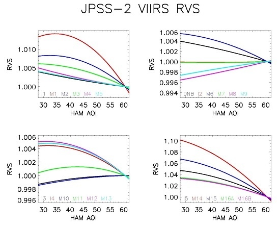
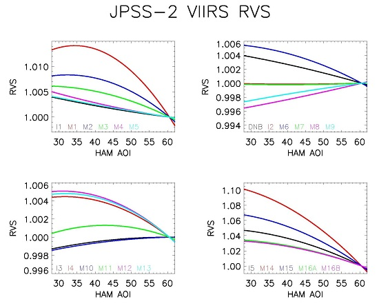
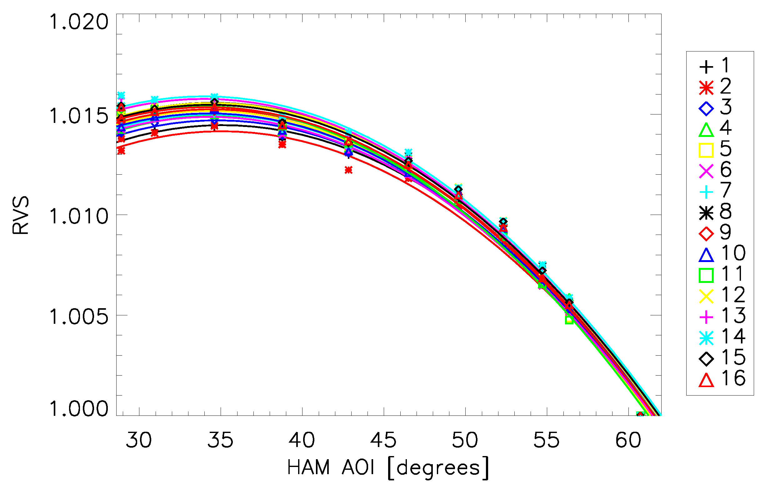
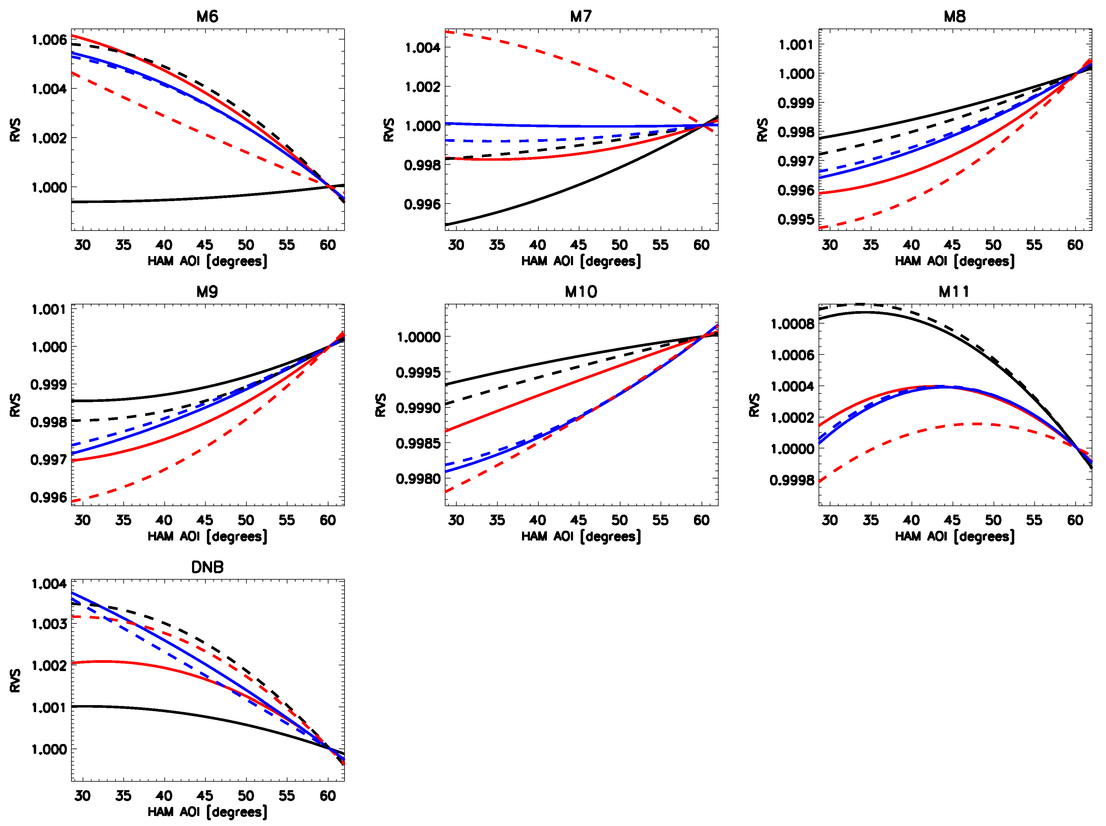
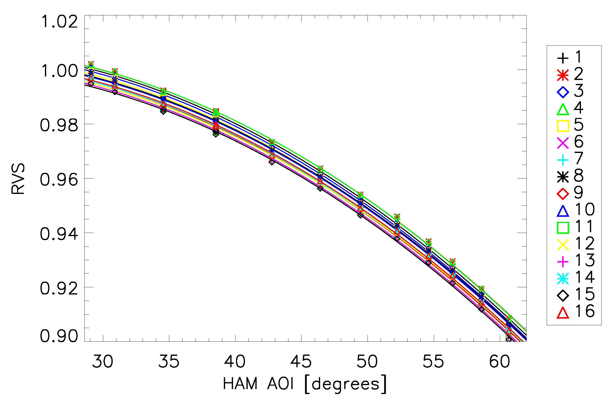
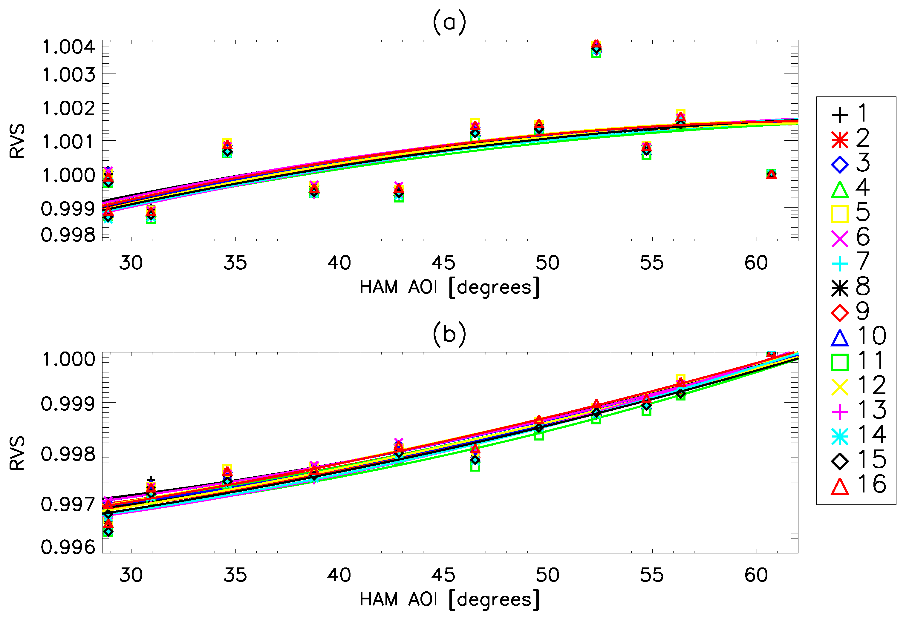
The RVS for all of the reflective bands and the DNB were fit using the approach outlined in Section 3 and [8]. Figure 1 shows an example of the un-normalized RVS fitting for band M1, HAM side A. The symbols represent the measured data and the lines denote the fit RVS functions. The RVS functions agree well with the measured data for band M1, and this is also the case for the remaining reflective bands. The derived RVS functions for all of the reflective bands and the DNB are shown in Figure 2 and Figure 3 for a middle detector. The blue curves denote the JPSS-2 RVS where solid and dashed lines indicate HAM sides A and B, respectively. In general, the RVS for the two HAM sides is very consistent for JPSS-2 VIIRS. In addition, for a given band, all detectors behave similarly (as seen in Figure 1 for band M1). The curves in Figure 2 and Figure 3 have been normalized to the AOI of 60.47 degrees. The largest RVS variation occurs for the bluest bands M1–M3 with up to about 1.5% change across the full range of AOI (from about 28.6 degrees to 60.5 degrees). The smallest RVS changes occur for bands M7, M11, and I2 with less than 0.1% variation over AOI. The atmospheric correction for M9 has been applied here but will be discussed in Section 4.3.
The RVS for SNPP and JPSS-1 VIIRS reflective bands and the DNB are also included in Figure 2 and Figure 3, represented by the black and red lines, respectively (again, solid and dashed lines indicate HAM sides A and B). The observed differences for all bands are in general small. The previous VIIRS builds had larger HAM side differences [8], particularly with bands M6 (for SNPP) and I2/M7 (for JPSS-1). The detector dependence for JPSS-2 VIIRS was also comparable for both SNPP and JPSS-1 VIIRS, with the exception of the DNB for which the edge detectors were outliers on earlier builds (particularly JPSS-1 VIIRS). The HAM coating was different for SNPP VIIRS; for JPSS-1 VIIRS, the HAM sides were coated at very different times [8].
4.2. Thermal Band Performance
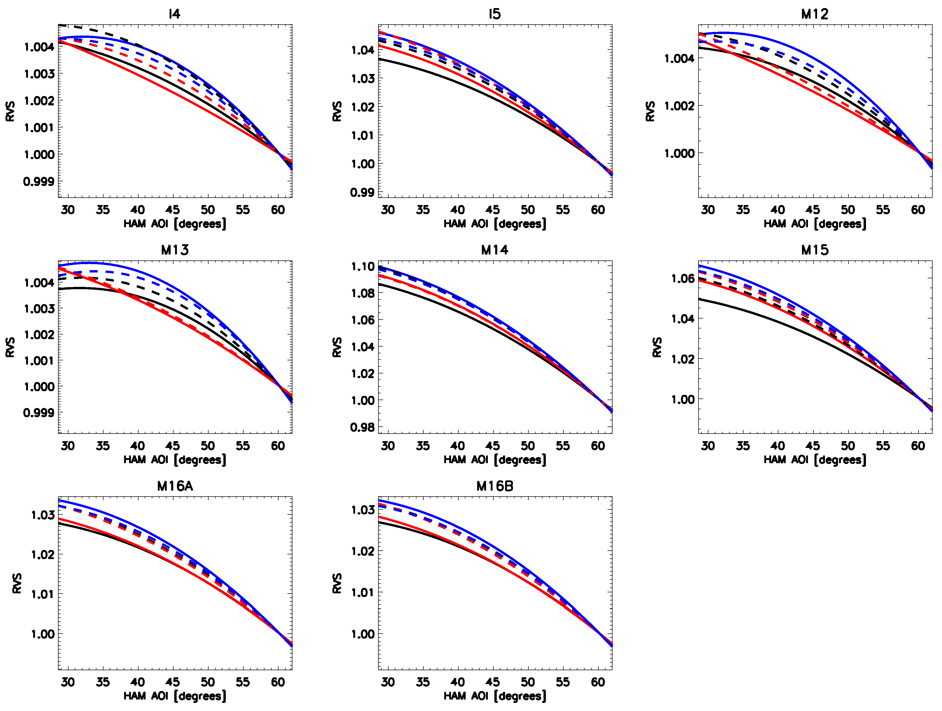
The relevant temperatures were extracted from VIIRS telemetry, and their corresponding radiances were calculated from the Planck equation, convolved over the spectral response functions. Then, the RVS in Equation (6) was calculated for each scan angle. These RVS values were used to conduct a fit versus HAM AOI (as determined from Equation (1)). The measured, un-normalized RVS along with the fitted curves for band M14 (HAM side A) are shown in Figure 4. The RVS function reproduces the measured data well for band M14, and this is also the case for the remaining thermal bands. Band M14 shows the greatest variation, changing by about 10% over the full AOI range. The derived RVS functions for all of the thermal bands are shown in Figure 5 for a middle detector. The blue curves denote the JPSS-2 RVS where solid and dashed lines indicate HAM sides A and B, respectively. The RVS in Figure 5 has been normalized to AOI (60.47 degrees). The other LWIR bands vary by between 3% and 6%; in contrast, the MWIR bands change by less than 1% across the full range of AOI. Very little HAM side or detector dependence was observed for any thermal band.
The SNPP and JPSS-1 thermal band RVS are also shown in Figure 5 by the black and red lines, respectively (again, solid and dashed lines indicate HAM sides A and B). In general, all bands behave in a similar manner. There is more HAM side variation on both SNPP and JPSS-1 compared to JPSS-2. In addition, the LWIR bands all show slightly larger RVS variation across the range of AOI compared to the previous builds. The MWIR bands show a comparable level of overall variation, but exhibit more curvature in the RVS function for JPSS-2 VIIRS.
4.3. Atmospheric Correction
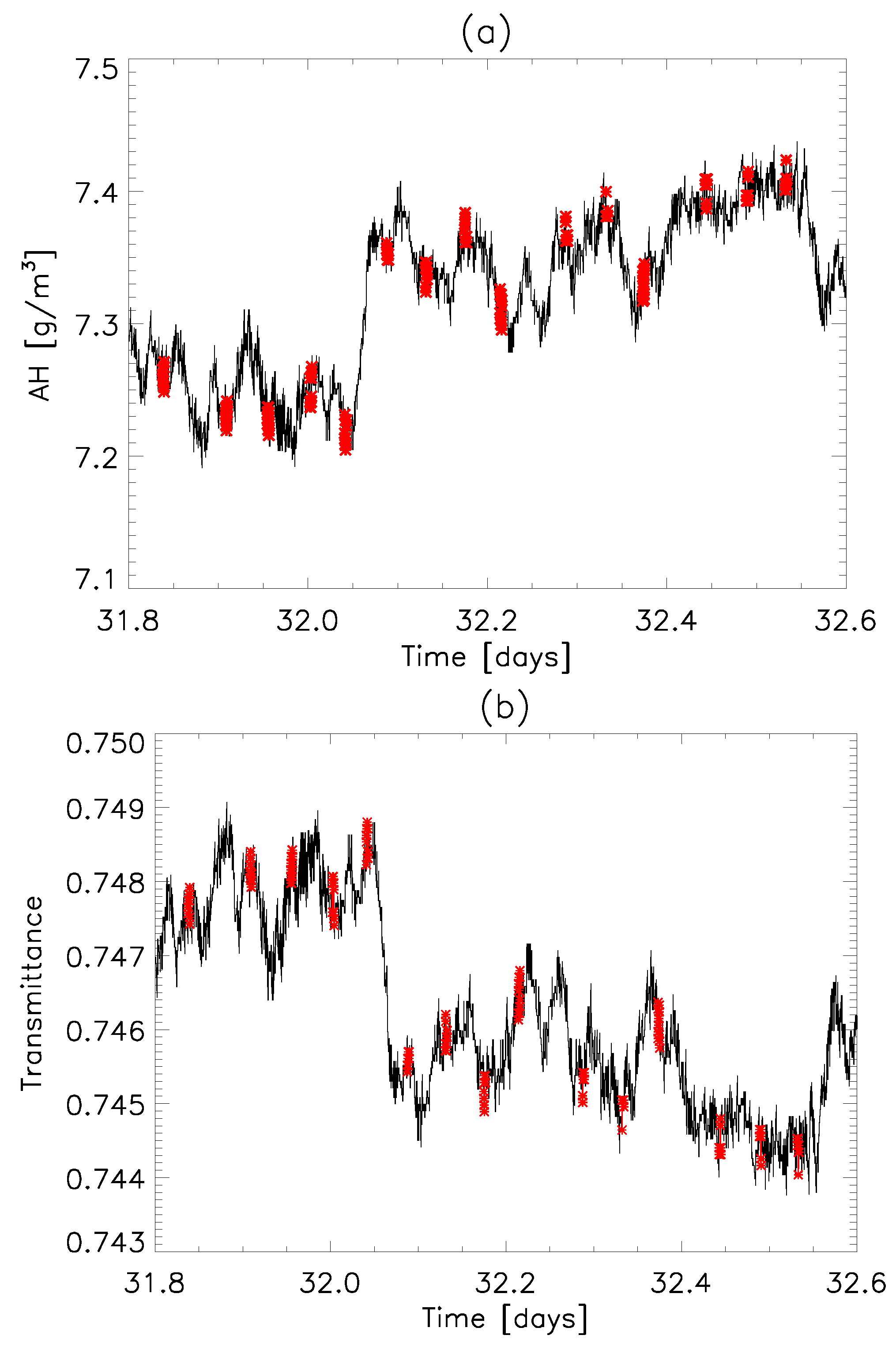
The calculated is plotted in Figure 6 using data from the THM that was close to the integrating sphere aperture. The black lines indicate all of the data taken over the course of the test while the red symbols represent the specific test data used in the RVS determination. There is a fair amount of variation in over all of the data (about 6%), but variations within the individual test data collections were small (below 0.4%).
UW provided the LBLRTM transmittance data convolved with a predicted M9 spectral response function. There are a number of narrow absorption lines within the M9 bandpass, making the estimate sensitive to the spectral response function used. The convolution was performed for all of the cases listed in Table 3. The atmospheric transmittance at a specific tend to zero as the path length increases in an exponential decay. The temperature dependence is subdominant to the and path length dependence. The model transmittances were then used to estimate the transmittance at the specific , temperature, and path length measured during the test. The estimates of are shown in Figure 6 for the duration of the testing. Again, the black lines indicate all of the data taken over the course of the test while the red symbols represent the specific test data collected for the RVS determination. The calculated transmittances were averaged over a particular test data collection and then applied to correct the measured sensor response. The atmospheric correction significantly reduced the apparent drift in the repeated measurements; the remaining drift was assumed to be linear and the same drift correction based on the repeated measurements was applied as used for the other reflective bands.
The fit RVS is shown in Figure 7 for HAM side A with and without the atmospheric correction (lower and upper plots). The curves in this figure are un-normalized. The data in the upper plot is much more scattered, while the atmospheric correction reduces the scatter significantly as seen in the lower plot. The fit reproduces the corrected data much better; all detectors behave in family. The HAM side difference for the normalized RVS for band M9 (middle detector) is shown in Figure 3. The solid line denotes HAM side A and the dashed line represents HAM side B; the observed differences are small. JPSS-1 VIIRS had a larger HAM side difference, while SNPP VIIRS had a similar amount of HAM side difference.
To quantify the improvement in the fitting, the root mean square (RMS) residuals for the fits with and without the atmospheric correction were 0.00025 and 0.00098; for comparison, the RMS residuals for neighboring bands (centered at 1260 nm and 1610 nm) were 0.00007 and 0.00023. As a check on the final band M9 RVS, a comparison between bands M8, M9, and M10 shows that the atmospheric corrected band M9 RVS behaves in family, as seen in Figure 3.
4.4. Uncertainty
The error sources for the measured reflective band RVS are the uncertainties in the response. Because this is a relative measurement, only the random error sources for the response contribute; thus, the uncertainty is taken to be the standard deviation of the mean over all measurements at a particular scan angle. Since the method of using linear interpolations was employed to remove the drift, the repeatability uncertainty was not estimated. For band M9, an additional uncertainty was estimated as the standard deviation of the mean for the atmospheric transmittance; then, the root sum square of this uncertainty and the response uncertainty was used as the measured RVS uncertainty.
To determine the uncertainty in the thermal band RVS, uncertainties in the individual contributions to the measured RVS needed to be estimated. The radiance uncertainty for each of the radiances that factor into the Equation (6) was determined to be the standard deviation of the radiance measurements over scan for each scan angle measurement. The uncertainty in the response was the random uncertainty in the background subtracted digital response; for the purposes of this work, the random error in and was the standard deviation of the mean over all measurements at a particular scan angle. A number of uncertainty contributors were not considered in the above sections because the RVS is a normalized quantity; as such, any term that is considered a bias to all measurements for a given band and detector will not contribute. Uncertainty contributors for the thermal bands that did not enter into this calculation include the temperature and spectral biases on the radiance uncertainty, the emissivity, and the reflectance of the RTA.
These uncertainties in the measured RVS for both the reflective and emissive bands were propagated through a least squares fitting routine, which provides estimates of the uncertainty on the fitting coefficients as well as covariances.
The final RVS uncertainty was estimated by propagating the coefficient uncertainties and covariances through Equation (12). An additional uncertainty on the AOI of the equivalent angular separation of one un-aggregated pixel was included. The covariant terms between the AOI uncertainty and the coefficient uncertainty were estimated by the Schwarz inequality; thus, the quoted uncertainty is a worst case. In practice, these terms are subdominant, so that the estimated uncertainty is expected to be close to the true uncertainty. The final uncertainty was then estimated for HAM AOI ranging from 28.6 degrees to 62 degrees, covering the full range of in orbit measurements.
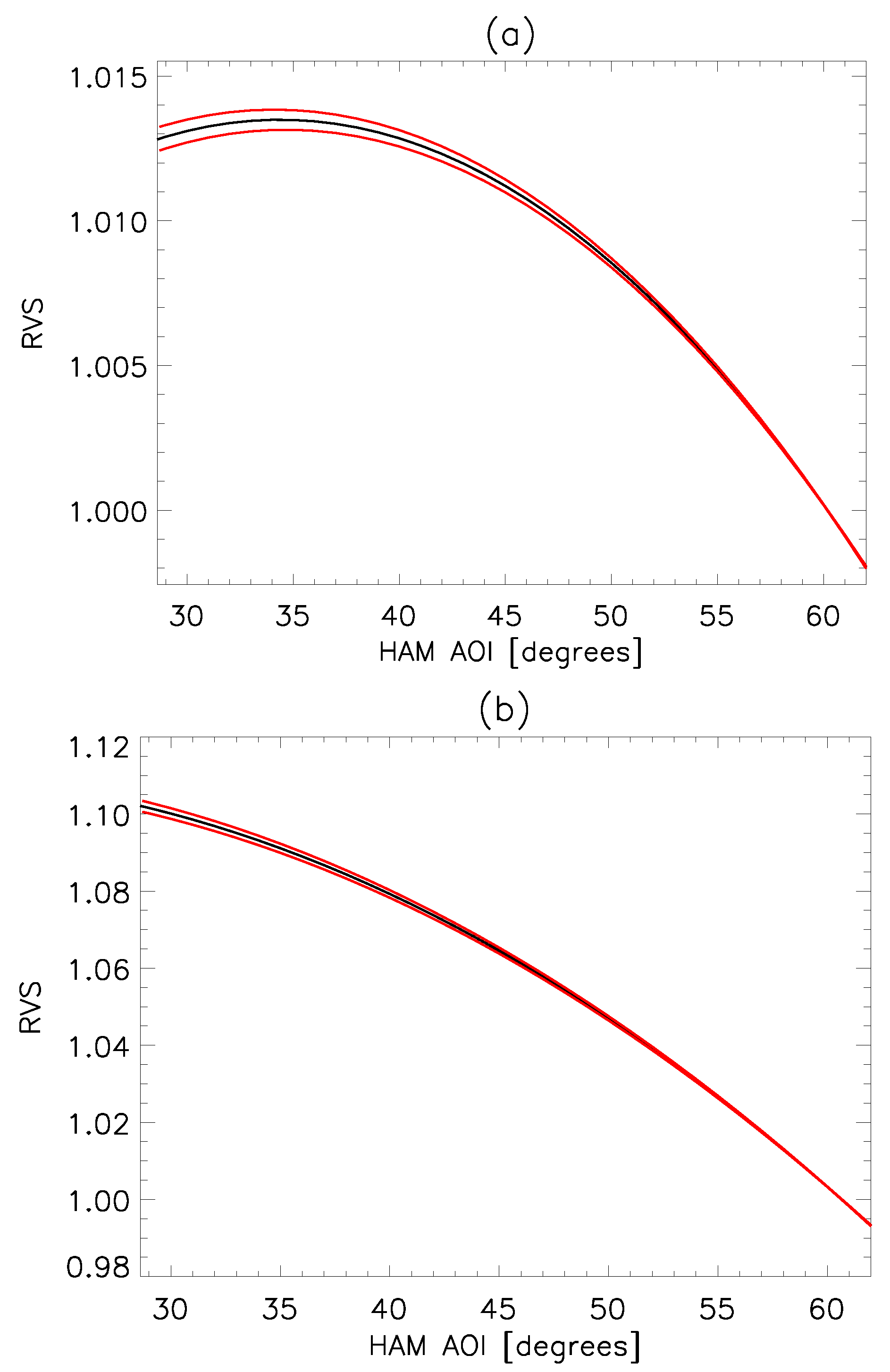
As an example, the uncertainty estimate for bands M1 and M14 are plotted with the RVS function in Figure 8. Note that the uncertainty is at a minimum near 60.5 degrees AOI, where the RVS is defined as unity. It is not exactly zero in this work because the Schwarz inequality was used and this provides an upper bound on the uncertainty. As expected, the uncertainty increases as one moves away from the normalization point and is the worst at the HAM minimum of about 28.7 degrees. This behavior is common to all bands.
For the reflective bands (I1–I3, M1–M11) and the DNB, maximum uncertainties range from about 0.009% for M10 to 0.05% for M4. This is below the target uncertainty of 0.3% allocated to the RVS by the sensor vendor as part of their total uncertainty budget. The band maximum uncertainties are listed in Table 4. For all bands, the largest contributions to the uncertainty are the and terms. As the RVS enters into the calibrated reflectance as a multiplicative factor for the reflective bands, the maximum uncertainty on the reflectance due to RVS for each band is equivalent to the maximum RVS uncertainties listed in Table 4.
For the thermal bands, the worst case uncertainties range from 0.11% for M15 to 0.26% for I4. Both I4 and I5 show uncertainties for some AOI that are above the 0.2% target value; all other bands are below their respective target values (0.2% for M12, M13, M15, and M16; 0.6% for M14). The larger uncertainties in bands I4 and I5 are driven by the uncertainties; these two bands are known to have higher noise (on the order of 3 times larger than the other thermal bands). The band maximum uncertainties are also listed in Table 4. For all of the thermal bands, the largest contributions to the uncertainty are the and terms. Propagating the maximum uncertainties listed in Table 4 to the retrieved brightness temperature yields the temperature uncertainties listed in Table 5. Brightness temperature uncertainties are generally around 0.1 K or lower, except at low scene temperatures (below 230 K for I4, M12 and M13; below 190 K for I5 and M14–M16). I5 has slightly higher uncertainties for most scene temperatures. Note that this is a worst case estimate near the end of a scan (where the HAM AOI is at a minimum).
4.5. Model Validity
The model simplifications outlined in Section 3.5 were used to reproduce the results in Section 4.1 and Section 4.2. In all cases, the differences between the two and three parameter fits defined by Equations (1) and (14) were negligible. The associated uncertainty for the two parameter RVS was also estimated. These uncertainties were slightly smaller than the estimates derived in Section 4.4 due mainly to reduction in covariant terms between the AOI uncertainty and the fitting coefficient uncertainty, whose contributions were subdominant but non-negligible.
5. Conclusions
The JPSS-2 VIIRS RVS is a critical parameter that must be characterized prior to launch in order to ensure accurate calibration once the instrument is on orbit. This parameter describes the relative variation in reflectance with scan angle for the fore-optics. Measurements were made in the summer of 2016 to characterize this quantity at the sensor vendor facility (Raytheon El Segundo). Analysis has shown less than 2% variation in the RVS for all reflective bands and mid-wave emissive bands, and between 3% and 10% variation in the RVS for the long-wave infrared. This is comparable to the two previous VIIRS builds, SNPP and JPSS-1. An atmospheric correction was applied to account for water vapor absorption in the laboratory environment. The measurement uncertainty was also estimated: up to 0.05% for the reflective bands and up to 0.26% for the thermal bands.
Acknowledgments
The authors would like to thank the following: the Raytheon test team including Tung Wang for conducting the performance tests and for developing much of the analysis methodology, and members of the government data analysis working group including James McCarthy for valuable comments. The above-mentioned provided valuable information and support to the analysis presented in this work.
Author Contributions
Jeff McIntire wrote the manuscript. Jeff McIntire performed the analysis contained in this work. David Moyer and Tiejun Chang independently verified the analysis contained in this work. Hassan Oudrari and Xiaoxiong Xiong contributed to the design of this study and to the development of the manuscript.
Conflicts of Interest
The authors declare no conflict of interest.
References
- McClain, C.; Hooker, S.; Feldman, G.; Bontempi, P. Satellite Data for Ocean Biology, Biogeochemistry, and Climate Research. EOS 2006, 87, 337–339. [Google Scholar] [CrossRef]
- King, M.D.; Menzel, W.P.; Kaufman, Y.J.; Tanre, D.; Gao, B.C.; Platnick, S.; Ackerman, S.A.; Remer, L.A.; Pincus, R.; Hubanks, P.A. Cloud and aerosol and water vapor properties, precipitable water, and profiles of temperature and humidity from MODIS. IEEE Trans. Geosci. Remote Sens. 2003, 41, 442–458. [Google Scholar] [CrossRef]
- Justice, C.O.; Vermote, E.; Townshend, J.R.G.; Defries, R.; Roy, D.P.; Hall, D.K.; Salomonson, V.V.; Privette, J.L.; Riggs, G.; Strahler, A.; et al. The Moderate Resolution Imaging Spectroradiometer (MODIS): Land remote sensing for global change research. IEEE Trans. Geosci. Remote Sens. 1998, 36, 1228–1249. [Google Scholar] [CrossRef]
- Xiong, X.; Butler, J.; Chiang, K.; Efremova, B.; Fulbright, J.; Lei, N.; McIntire, J.; Oudrari, H.; Wang, Z.; Wu, A. Assessment of S-NPP VIIRS On-Orbit Radiometric Calibration and Performance. Remote Sens. 2016, 8, 84. [Google Scholar] [CrossRef]
- Cao, C.; De Luccia, F.; Xiong, X.; Wolfe, R.; Weng, F. Early in orbit performance of the Visible Infrared Imaging Radiometer Suite (VIIRS) onboard the Suomi National Polar-Orbiting Partnership (S-NPP) satellite. IEEE Trans. Geosci. Remote Sens. 2014, 52, 1142–1156. [Google Scholar] [CrossRef]
- Oudrari, H.; McIntire, J.; Xiong, X.; Butler, J.; Ji, Q.; Schwarting, T.; Lee, S.; Efremova, B. JPSS-1 VIIRS Radiometric Characterization and Calibration Based on Pre-Launch Testing. Remote Sens. 2016, 8, 41. [Google Scholar] [CrossRef]
- Oudrari, H.; McIntire, J.; Xiong, X.; Butler, J.; Lee, S.; Lei, N.; Schwarting, T.; Sun, J. Prelaunch Radiometric Characterization and Calibration of the S-NPP VIIRS Sensor. IEEE Trans. Geosci. Remote Sens. 2015, 53, 2195–2210. [Google Scholar] [CrossRef]
- Moyer, D.; McIntire, J.; Oudrari, H.; McCarthy, J.; Xiong, X.; DeLuccia, F. JPSS-1 VIIRS Pre-Launch Response Versus Scan Angle Testing and Performance. Remote Sens. 2016, 8, 141. [Google Scholar] [CrossRef]
- McIntire, J.; Moeller, C.; Oudrari, H.; Xiong, X. Atmospheric Correction for JPSS-2 VIIRS Response versus Scan Angle Measurements. In Proceedings of the Earth Observing Systems XXII, San Diego, CA, USA, 6–10 August 2017; Volume 10402. [Google Scholar]
- McIntire, J.; Moyer, D.; Oudrari, H.; Xiong, X. Pre-Launch Radiometric Characterization of JPSS-1 VIIRS Thermal Emissive Bands. Remote Sens. 2016, 8, 47. [Google Scholar] [CrossRef]
- Lawrence, M.G. The relationship between relative humidity and the dewpoint temperature in moist air: A simple conversion and applications. Am. Meterol. Soc. 2005, 86, 225–233. [Google Scholar] [CrossRef]
- Young, J.B. Atmospheric Transmittance Effects on Calibration; Technical Report; Santa Barbara Research Center: Santa Barbara, CA, USA, 1995. [Google Scholar]
- Clough, S.A.; Shephard, M.W.; Mlawer, E.J.; Delamere, J.S.; Iacono, M.J.; Cady-Pereira, K.; Boukabara, S.; Brown, P.D. Atmospheric radiative transfer modeling: A summary of the AER codes, Short Communication. J. Quant. Spectrosc. Radiat. Transf. 2005, 91, 233–244. [Google Scholar] [CrossRef]
- Clough, S.A.; Iacono, M.J.; Moncet, J.L. Line-by-line calculation of atmospheric fluxes and cooling rates: Application to water vapor. J. Geophys. Res. 1992, 97, 15761–15785. [Google Scholar] [CrossRef]
- Taylor, J.R. An Introduction to Error Analysis; University Science Books: Sausalito, CA, USA, 1997. [Google Scholar]
- Taylor, B.N.; Kuyatt, C.E. Guidelines for Evaluating and Expressing the Uncertainty of NIST Measurement Results; National Institute of Standards and Technology (NIST): Gaithersburg, MD, USA, 1994.
Figure 1.
Band M1 un-normalized RVS plotted as a function of HAM AOI for HAM side A. The legend defines the different symbol/color combinations that correspond to each detector.
Figure 1.
Band M1 un-normalized RVS plotted as a function of HAM AOI for HAM side A. The legend defines the different symbol/color combinations that correspond to each detector.

Figure 2.
SNPP, JPSS-1, and JPSS-2 reflective band (I1–I3 and M1–M5) RVS plotted versus HAM AOI (black, red, and blue lines respectively). Solid and dashed lines denote HAM sides A and B, respectively.
Figure 2.
SNPP, JPSS-1, and JPSS-2 reflective band (I1–I3 and M1–M5) RVS plotted versus HAM AOI (black, red, and blue lines respectively). Solid and dashed lines denote HAM sides A and B, respectively.
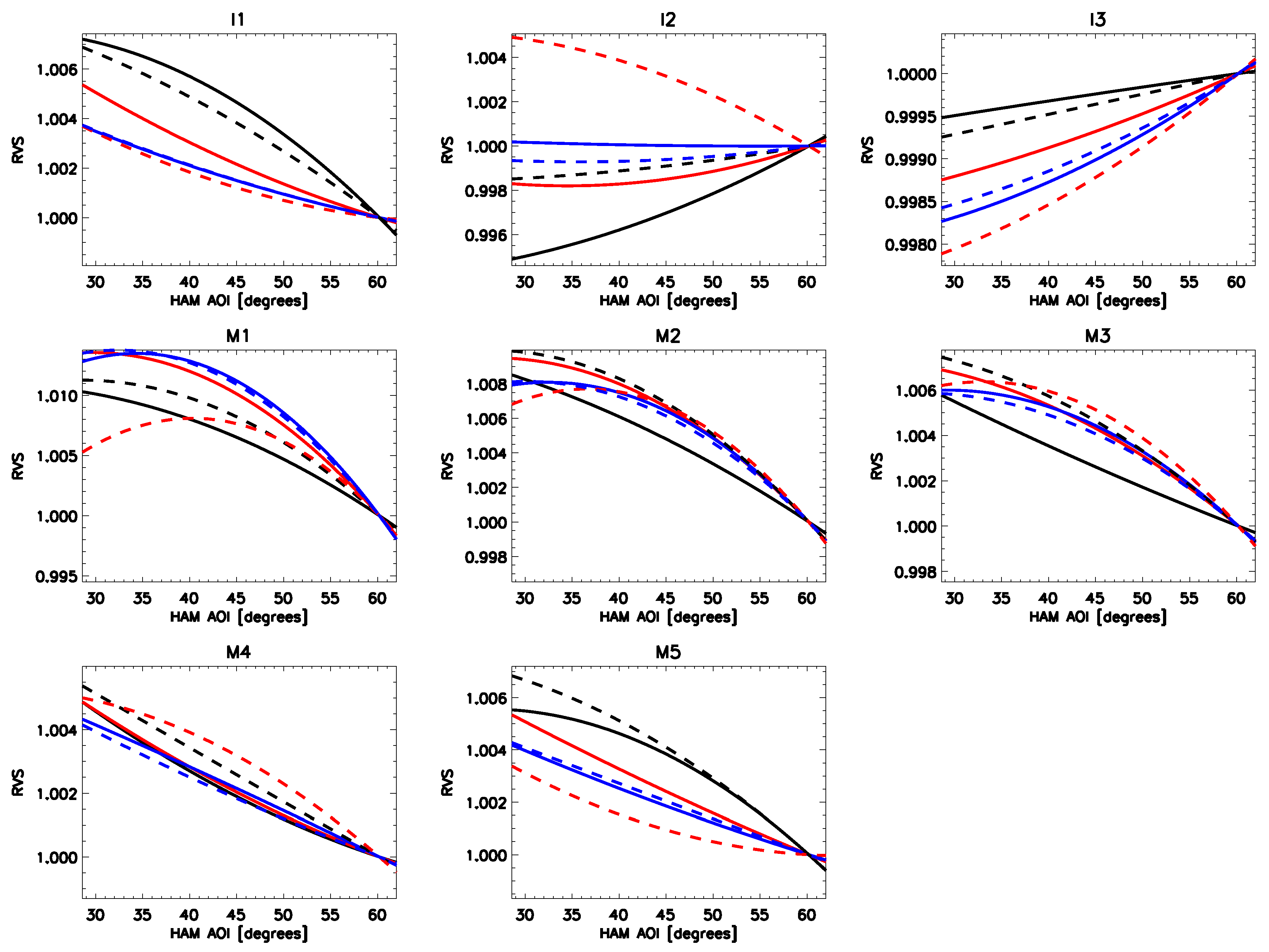
Figure 3.
SNPP, JPSS-1, and JPSS-2 reflective band (M6–M11) and DNB RVS plotted versus HAM AOI (black, red, and blue lines respectively). Solid and dashed lines denote HAM sides A and B, respectively.
Figure 3.
SNPP, JPSS-1, and JPSS-2 reflective band (M6–M11) and DNB RVS plotted versus HAM AOI (black, red, and blue lines respectively). Solid and dashed lines denote HAM sides A and B, respectively.

Figure 4.
Band M14 un-normalized RVS plotted as a function of HAM AOI for HAM side A. The legend defines the different symbol/color combinations that correspond to each detector.
Figure 4.
Band M14 un-normalized RVS plotted as a function of HAM AOI for HAM side A. The legend defines the different symbol/color combinations that correspond to each detector.

Figure 5.
SNPP, JPSS-1, and JPSS-2 thermal band RVS plotted versus HAM AOI (black, red, and blue lines respectively). Solid and dashed lines denote HAM sides A and B, respectively.
Figure 5.
SNPP, JPSS-1, and JPSS-2 thermal band RVS plotted versus HAM AOI (black, red, and blue lines respectively). Solid and dashed lines denote HAM sides A and B, respectively.

Figure 6.
(a) plotted versus days since the beginning of July 2016; (b) atmospheric transmittance plotted versus days since the beginning of July 2016. Black lines indicate all data taken over the course of testing; red symbols represent data used in the determination of the reflective band RVS.
Figure 6.
(a) plotted versus days since the beginning of July 2016; (b) atmospheric transmittance plotted versus days since the beginning of July 2016. Black lines indicate all data taken over the course of testing; red symbols represent data used in the determination of the reflective band RVS.

Figure 7.
Band M9 un-normalized RVS plotted as a function of HAM AOI for HAM side A without (a) and with (b) the atmospheric correction. The legend defines the different symbol/color combinations that correspond to each detector.
Figure 7.
Band M9 un-normalized RVS plotted as a function of HAM AOI for HAM side A without (a) and with (b) the atmospheric correction. The legend defines the different symbol/color combinations that correspond to each detector.

Figure 8.
Plots of band M1 (a) and M14 (b) RVS for a middle detector, HAM side A with their corresponding uncertainty estimates (in red) as a function of HAM AOI.
Figure 8.
Plots of band M1 (a) and M14 (b) RVS for a middle detector, HAM side A with their corresponding uncertainty estimates (in red) as a function of HAM AOI.


Table 1.
VIIRS spectral bands along with their center wavelengths.
| Band | Center (nm) | Band | Center (nm) | Band | Center (nm) |
|---|---|---|---|---|---|
| M1 | 412 | M7 | 865 | I4 | 3740 |
| M2 | 445 | I2 | 865 | M13 | 4050 |
| M3 | 488 | M8 | 1240 | M14 | 8550 |
| M4 | 555 | M9 | 1378 | M15 | 10,763 |
| I1 | 640 | M10 | 1610 | I5 | 11,450 |
| M5 | 672 | I3 | 1610 | M16A | 12,013 |
| DNB | 700 | M11 | 2250 | M16B | 12,013 |
| M6 | 746 | M12 | 3700 |
Table 2.
Scan angles measured for both the reflective and emissive RVS testing in the order measured, along with their corresponding HAM AOI. All angles are given in degrees and are referenced to the boresight, which is about 0.6 degrees from band M1 pointing.
Table 2.
Scan angles measured for both the reflective and emissive RVS testing in the order measured, along with their corresponding HAM AOI. All angles are given in degrees and are referenced to the boresight, which is about 0.6 degrees from band M1 pointing.
| Reflective | Thermal | ||||
|---|---|---|---|---|---|
| Collection | Scan Angle (Degrees) | HAM AOI (Degrees) | Collection | Scan Angle (Degrees) | HAM AOI (Degrees) |
| 1 | −66.3 | 60.7 | 1 | −8.0 | 38.5 |
| 2 | −8.7 | 38.8 | 2 | −66.2 | 60.7 |
| 3 | −38.7 | 49.6 | 3 | 21.6 | 30.9 |
| 4 | 5.3 | 34.6 | 4 | −45.5 | 52.2 |
| 5 | −45.7 | 52.3 | 5 | 5.5 | 34.5 |
| 6 | −8.7 | 38.8 | 6 | −8.0 | 38.5 |
| 7 | −55.7 | 56.4 | 7 | −55.9 | 56.4 |
| 8 | 21.3 | 30.9 | 8 | −20.5 | 42.8 |
| 9 | −30.7 | 46.5 | 9 | −38.5 | 49.5 |
| 10 | −8.7 | 38.6 | 10 | −8.0 | 38.5 |
| 11 | −51.7 | 54.7 | 11 | −51.4 | 54.6 |
| 12 | 37.5 | 28.9 | 12 | 35.0 | 29.1 |
| 13 | −20.7 | 42.8 | 13 | −30.5 | 46.4 |
| 14 | 54.5 | 28.9 | 14 | −8.0 | 38.5 |
| 15 | −8.7 | 38.8 | 15 | −61.2 | 58.6 |
| 16 | 5.4 | 34.6 |
Table 3.
Input parameters used in the LBLRTM. All permutations of these input parameters were used in the model calculations.
Table 3.
Input parameters used in the LBLRTM. All permutations of these input parameters were used in the model calculations.
| (g/m) | T (K) | ℓ (m) |
|---|---|---|
| 2.5, 5, 7.5, | 290, 305, | 1, 3, 4.5, 6, 9, 12, 20, |
| 10, 12.5, 15 | 320 | 27.5, 35, 42.5, 50, 75 |
Table 4.
Band maximum RVS uncertainty estimate for all VIIRS bands (in %).
| Band | Uncertainty | Band | Uncertainty | Band | Uncertainty |
|---|---|---|---|---|---|
| M1 | 0.041 | M7 | 0.016 | I4 | 0.263 |
| M2 | 0.026 | I2 | 0.017 | M13 | 0.152 |
| M3 | 0.025 | M8 | 0.013 | M14 | 0.130 |
| M4 | 0.053 | M9 | 0.021 | M15 | 0.113 |
| I1 | 0.015 | M10 | 0.009 | I5 | 0.230 |
| M5 | 0.035 | I3 | 0.026 | M16A | 0.113 |
| DNB | 0.010 | M11 | 0.016 | M16B | 0.114 |
| M6 | 0.023 | M12 | 0.167 |
Table 5.
Brightness temperature uncertainties due solely to the RVS maximum uncertainties listed in Table 4 (in K).
Table 5.
Brightness temperature uncertainties due solely to the RVS maximum uncertainties listed in Table 4 (in K).
| Scene T | I4 | I5 | M12 | M13 | M14 | M15 | M16A | M16B |
|---|---|---|---|---|---|---|---|---|
| 190 | 0.65 | 0.43 | 0.35 | 0.40 | 0.40 | 0.23 | 0.21 | 0.21 |
| 210 | 0.71 | 0.23 | 0.38 | 0.44 | 0.18 | 0.12 | 0.12 | 0.12 |
| 230 | 0.51 | 0.14 | 0.30 | 0.23 | 0.08 | 0.06 | 0.06 | 0.06 |
| 250 | 0.15 | 0.07 | 0.08 | 0.08 | 0.04 | 0.03 | 0.03 | 0.03 |
| 270 | 0.04 | 0.04 | 0.02 | 0.02 | 0.02 | 0.02 | 0.02 | 0.02 |
| 290 | 0.05 | 0.07 | 0.03 | 0.03 | 0.03 | 0.03 | 0.03 | 0.03 |
| 310 | 0.07 | 0.10 | 0.05 | 0.04 | 0.05 | 0.05 | 0.05 | 0.05 |
| 330 | 0.08 | 0.13 | 0.05 | 0.05 | 0.06 | 0.06 | 0.06 | 0.06 |
| 345 | 0.09 | 0.15 | 0.06 | 0.06 | 0.08 | 0.07 | 0.08 | 0.08 |
© 2017 by the authors. Licensee MDPI, Basel, Switzerland. This article is an open access article distributed under the terms and conditions of the Creative Commons Attribution (CC BY) license (http://creativecommons.org/licenses/by/4.0/).
Share and Cite
MDPI and ACS Style
McIntire, J.; Moyer, D.; Chang, T.; Oudrari, H.; Xiong, X. Pre-Launch JPSS-2 VIIRS Response versus Scan Angle Characterization. Remote Sens. 2017, 9, 1300. https://doi.org/10.3390/rs9121300
AMA Style
McIntire J, Moyer D, Chang T, Oudrari H, Xiong X. Pre-Launch JPSS-2 VIIRS Response versus Scan Angle Characterization. Remote Sensing. 2017; 9(12):1300. https://doi.org/10.3390/rs9121300
Chicago/Turabian StyleMcIntire, Jeff, David Moyer, Tiejun Chang, Hassan Oudrari, and Xiaoxiong Xiong. 2017. "Pre-Launch JPSS-2 VIIRS Response versus Scan Angle Characterization" Remote Sensing 9, no. 12: 1300. https://doi.org/10.3390/rs9121300
Note that from the first issue of 2016, this journal uses article numbers instead of page numbers. See further details here.