Article

Geo-Parcel Based Crop Identification by Integrating High Spatial-Temporal Resolution Imagery from Multi-Source Satellite Data

1
Institute of Remote Sensing and Digital Earth, Chinese Academy of Sciences, Beijing 100101, China
2
University of Chinese Academy of Sciences, Beijing 100049, China
3
Agricultural Science and Technology Information Research Institute, Guangxi Academy of Agricultural Sciences, Nanning 530007, China
4
College of Computer Science and Technology, Zhejiang University of Technology, Hangzhou 310014, China
5
Department of Mathematics and Information Science, College of Science, Chang’an University, Xi’an 710064, China
*
Author to whom correspondence should be addressed.
Remote Sens. 2017, 9(12), 1298; https://doi.org/10.3390/rs9121298
Submission received: 21 October 2017 / Revised: 8 December 2017 / Accepted: 8 December 2017 / Published: 12 December 2017
(This article belongs to the Section Remote Sensing in Agriculture and Vegetation)

Abstract

:
Geo-parcel based crop identification plays an important role in precision agriculture. It meets the needs of refined farmland management. This study presents an improved identification procedure for geo-parcel based crop identification by combining fine-resolution images and multi-source medium-resolution images. GF-2 images with fine spatial resolution of 0.8 m provided agricultural farming plot boundaries, and GF-1 (16 m) and Landsat 8 OLI data were used to transform the geo-parcel based enhanced vegetation index (EVI) time-series. In this study, we propose a piecewise EVI time-series smoothing method to fit irregular time profiles, especially for crop rotation situations. Global EVI time-series were divided into several temporal segments, from which phenological metrics could be derived. This method was applied to Lixian, where crop rotation was the common practice of growing different types of crops, in the same plot, in sequenced seasons. After collection of phenological features and multi-temporal spectral information, Random Forest (RF) was performed to classify crop types, and the overall accuracy was 93.27%. Moreover, an analysis of feature significance showed that phenological features were of greater importance for distinguishing agricultural land cover compared to temporal spectral information. The identification results indicated that the integration of high spatial-temporal resolution imagery is promising for geo-parcel based crop identification and that the newly proposed smoothing method is effective.

Graphical Abstract

1. Introduction

With the development of agricultural management, agro-ecology studies and agricultural policy making, especially in precision agriculture, there have been increasing demands for crop distribution information on a land plot scale. Field survey methods to acquire crop types are time-consuming and laborious. In contrast, remote sensing has been widely used in agricultural management because it can be effectively applied on a large scale. However, due to being limited by data acquisition and satellite reception issues, remote sensing imagery has difficulty supplying high spatial and high temporal resolution at the same time.
A number of studies have identified different crops, based on their phenology, using high temporal resolution satellite data, particularly from coarse-resolution images, such as those from Advanced Very High Resolution Radiometer (AVHRR) and Moderate Resolution Imaging Spectroradiometer (MODIS). With a short revisit interval, they help to continuously observe land cover changes and detect vegetation phenological development. Many studies focused on constructing a vegetation index (VI) time-series using these kinds of images. Reed et al. [1] derived a suite of 12 metrics from 4 years of AVHRR normalized difference vegetation index (NDVI) time-series, and they found that the metrics were strongly consistent with various land cover types and their predicted phenological characteristics. Hill et al. [2] disaggregated quantitative metrics from AVHRR NDVI time-series for 8 years, analyzed the temporal and spatial patterns of key NDVI metrics, and made classifications. Sibanda et al. [3] derived phenological metrics from a 16-day MODIS NDVI time-series, compared the greenness change rate of cotton, maize and sorghum over the onset of green-up, green-peak and the senescence growth period, and significantly (p < 0.05) distinguished cotton fields from maize and sorghum fields. As shown above, the vegetative index (VI) time-series can apparently respond to vegetative phenology. However, due to the sensor observation angle, response accuracy, sunlight conditions, cloudy weather and atmospheric factors, the VI time-series showed an irregular status, which made it difficult to extract phenological metrics. Many studies have proposed various VI smoothing methods, and the commonly used VI curve filtering methods are the Best Index Slope Extraction Method (BISE) [4], Mean Value Iteration (MVI) [5], Savitzky–Golay Filter (S–G) [6], Asymmetric Gaussian Fitting (AG) [7], Whittaker smoother (WT) [8] and Double Logistic function fitting algorithm (DL) [9]. Hird et al. [10] selected six kinds of NDVI filtering methods for a quantitative comparative analysis and explained that the purpose of filtering was to maximize the elimination of abnormal impacts while maintaining true values. These existing methods have been applied to smooth VI time-series and eliminate unnecessary fluctuations, especially for crop single growth seasons. However, crop rotation practices demand a smoothing method for fitting a time profile with multiple peaks. Our study presents an adaptive smoothing method for identifying crop rotations.
Although it is advantageous to form continuous observations of land cover using coarse-resolution images, because of low spatial resolution and resulting mixed pixels, pixel-based analyses often lead to inaccurate results. Consequently, coarse-spatial resolution is unsuitable for identifying crops in small agricultural field plots that have high spatial heterogeneity. With the development of high-resolution technology at the beginning of 21st century, high spatial resolution images, such as images from SPOT-5, IKONOS, and Worldview satellite, are capable of depicting detailed geometric and textural information, which is often negligible in low- and medium-resolution images. Turker et al. [11] identified geo-parcel based crop types separately, using SPOT-4, SPOT-5, IKONOS and Quickbird images for similar climatic conditions, and they compared the classification accuracies between filtered and unfiltered images. As a whole, the resulting accuracies were above 83%. Immitzer et al. [12] used the Random Forest algorithm to classify 10 tree species in Austria, using high spatial resolution imagery, Worldview-2 with eight bands, and an overall accuracy of approximately 82%. To effectively utilize the geometric/textual information of high-resolution imagery, the object-based analysis method was developed. The performances of pixel-based versus object-based approaches were compared by many studies, and scholars found that the latter approach outperformed the former approach [13]. However, the revisit cycle of high spatial resolution imagery is too long to capture the optimal phase for crop identification, not mentioning the frequent interference of cloud cover during the acquisition time.
The contradiction between the spatial and temporal resolutions of single-source satellite data may limit its potential for many applications that demand observations with high spatial and temporal resolution. To overcome the limits of single-source data, a trend of synchronously utilizing data from multiple satellite sensors has recently been observed. One of these types of techniques is Spatial and Temporal Data Fusion (STDF), which aims to construct relatively intensive time-series imagery with fine spatial resolution by blending coarse and fine spatial resolution images [14,15,16]. Hilker et al. [15] used the Spatial and Temporal Adaptive Reflectance Fusion Model (STARFM) to blend Landsat images with MODIS data for crop monitoring in central British Columbia, Canada. In their study, 18 synthetic time-series Landsat images were obtained using the STARFM algorithm, and the results showed that the crop growing patterns can be captured well by the synthetic time-series data. However, resolutions of these Landsat-like synthetic images are still relatively coarse (mostly 30 m resolution), and they are mainly used for pixel-based applications. Recently, some object-based STDF methods were proposed, which integrate objects segmented from high-resolution imagery with spectral/temporal information from coarse imagery. In a study of crop rotation classification, Conrad et al. [17] extracted the land plot objects through segmenting the SPOT-5 data and then assigned tasseled cap indices, derived from the bi-temporal ASTER images, to these objects. Their results demonstrated the effectiveness of this method. Singha et al. [18] obtained synthetic time-series dataset with a 16-day revisiting cycle and 30 m spatial resolution from MODIS and HJ-1 A/B CCD by using the STARFM algorithm and used a multi-resolution segmentation algorithm on an HJ-1 dataset to acquire objects. After the selection of key temporal features, a decision tree classifier produced a satisfactory performance (overall accuracy of >84%) in paddy rice mapping. Although the object-based STDF methods could achieve relatively high accuracy in crop identification, objects that were segmented from imagery, in the abovementioned resolution, may be inconsistent with the real boundaries of farm land plots, and the only single sensor for medium-resolution data may lead to insufficient temporal coverage. Therefore, higher-resolution spatial and temporal data from multi-source data should be integrated, to improve the geometric accuracy of land plot objects and expand the temporal observation cover range.
This paper aimed to solve the limitations of single-source satellite data in geo-parcel based crop identification. Fine spatial resolution images with 0.8 m spatial resolution from the GF-2 satellite were used to obtain precise agricultural field plots, which were considered to be the smallest analytical elements. Multi-source medium-resolution data from GF-1 and Landsat 8 OLI were utilized together, in order to acquire intensive observations. To improve the EVI time profile fitting effect, we developed a piecewise EVI time-series smoothing method that worked well, especially for rotated crop cases. Then, we constructed a feature set that contained phenological metrics that were derived from the smoothed EVI time profile, and multi-temporal spectral features, and made classifications using Random Forest. The results showed that the proposed piecewise fitting method performed better than the S–G and the Harmonic Analysis of Time Series (HANTS) methods for crop classification, and the integration of the two kinds of features could significantly improve classification accuracy.

2. Materials and Methods

2.1. Study Area

Lixian, with an area of 2107.3 km2, is located in the northwest part of the Hunan Province (Figure 1). It is named after Lishui River, which flows through the entire territory. Its middle part is situated in the largest plain in Hunan, the famous Liyang Plain, and the northwest part of the province is mountainous. It has a subtropical humid monsoon climate, with an average temperature and rich water resources. The average annual temperature is 16.7 °C, and the annual precipitation is 1200 to 1900 mm. The climatic conditions are suitable for crop growth, including rice, cotton and cole crops.

2.2. Data

2.2.1. Remotely Sensed Imagery

Two disparate spatial resolution images were used in our study. One of them was fine spatial resolution imagery, obtained from GF-2 satellite data. Due to its narrow width of 45 km, 12 images in total covered the study area completely. The Gram–Schmidt Pan Sharpening method was used to sharpen multispectral (4 m) bands using high-resolution panchromatic (1 m) bands. This created a high-resolution multispectral GF-2 dataset, and the resolution of sub-satellite points reached 0.8 m. Then, Landsat 8/OLI imagery, provided by the United States Geological Survey (USGS), was used as reference data during orthorectification and geometric correction. The second-order polynomial interpolation method was used, and approximately 50 ground control points were selected for precise geometric registration, resulting in a controlled correction error within 0.5 pixels.
The medium-resolution imagery was mainly from the GF-1 WFV (Wide Field View) sensors. Four WFV sensors had the ability of acquiring imagery with 16 m spatial resolution and a four-day revisit cycle. The spectral bands ranged from visible to near-infrared wavelengths. Technical specification of the GF1 dataset is provided in Table 1. Due to cloudy and rainy weather, valid GF-1 images were always insufficient in continuous observation, as shown in Table 2. To construct intensive time-series, Landsat 8 OLI multispectral bands were used as supplementary data when a critical phase for crop identification was missing or key time point should be caught. Table 1 lists the medium-resolution data that were used in the experiment.

2.2.2. Ancillary Data

Digital elevation model (DEM) data were used for the orthorectification of GF-1 data. To assist with crop classification and accuracy assessment of the classification results, an extensive field survey was conducted in March, August and November 2016. Samples from 500 farming plots were collected using GPS to record their geometric positions. Other ancillary data, including administrative boundaries, road networks, and phenological information about crops, were also collected.

2.3. Methods

To identify farmland crop types, much pre-processing work on multi-source satellite data was done. We proposed a piecewise EVI time profile smoothing method for fitting the EVI time series, and we made classifications using a Random Forest classifier.
The workflow of the farmland-based crop mapping method is shown in Figure 2.

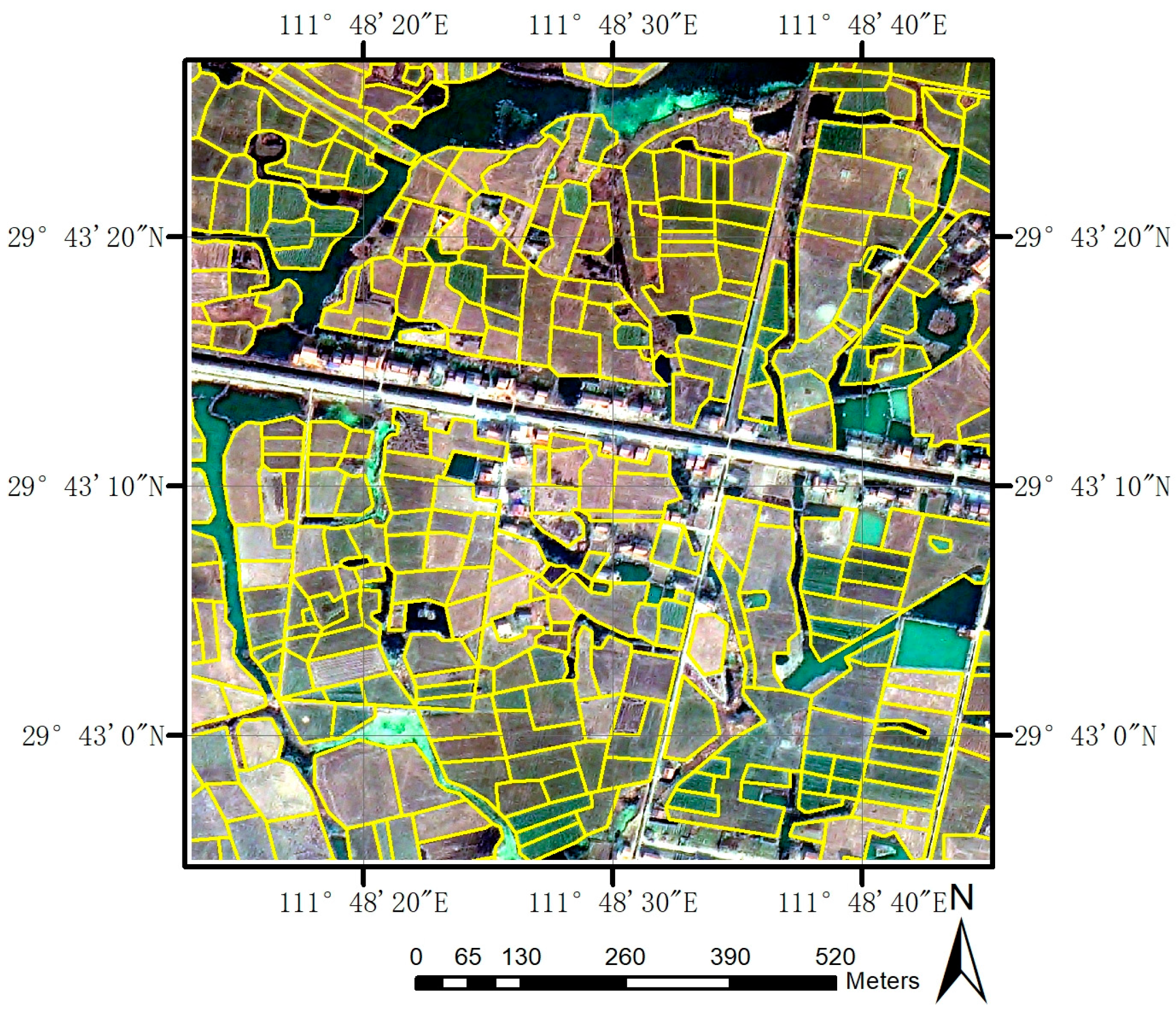
2.3.1. Geo-Parcels Extraction

The first step of the object-based STDF analysis involves object extraction to produce separate and homogenous geo-parcels. Geo-parcel extraction was based on GF-2 0.8 m fusion data, which accurately depicted the surface information in detail (Figure 3). It was performed manually along the real boundaries of farm land plots, as shown in the image. Each plot was considered to be the smallest analytical element. The total number of geo-parcels was approximately 590,000.

2.3.2. Pre-Processing of Medium-Resolution Images

GF-1 WFV data were radiometrically calibrated, atmospherically corrected, orthorectified and accurately geographically registered. The geographic correction used Landsat 8 OLI imagery as a reference, making the correction error controlled within 0.5 pixels. Landsat 8 OLI images were also radiometrically calibrated and atmospherically corrected. We used the FLAASH module in ENVI software for the atmospheric correction of the Landsat 8 OLI images. After that, image sharpening was applied to OLI images, using panchromatic and multispectral bands, which produced images with 15 m resolution. Due to the sensor performance and satellite imaging pose, it is essential to normalize different sensors in radiometric features. Radiometric inter-calibration was performed, using the method presented by Huang et al. [19]. The surface reflectance of other GF-1 WFV sensors and OLI was calibrated, using the reflectance of the GF-1 WFV1 sensor. Satellite images had many invalid pixels caused by cloudy and hazy weather conditions. Discarding the invalid pixels might lead to an inadequate observation frequency when constructing VI time-series. The strategy adopted here was to remove cloud and haze parts, fragment images and preserve the valid parts.

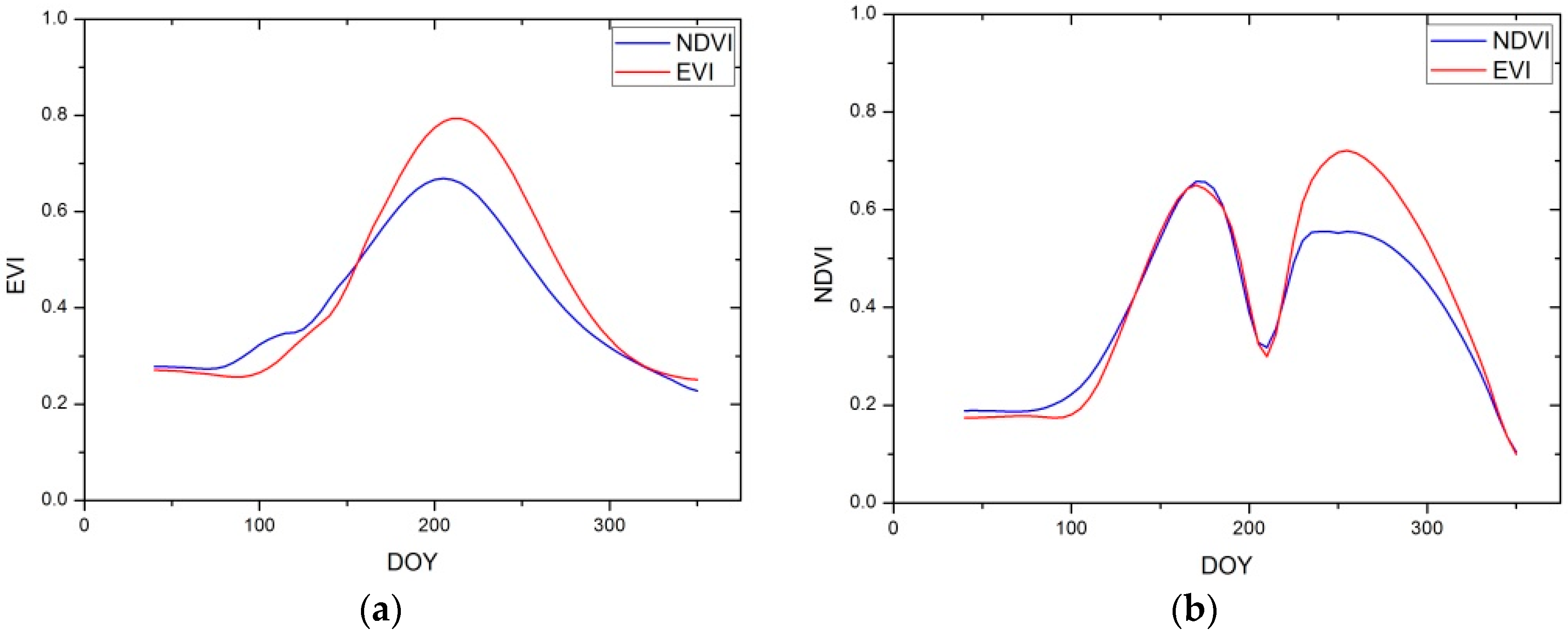
2.3.3. Construction of the Vegetation Index Time-Series

The VI time-series fluctuates according to physiological states during growing stages. Land cover types can be identified by analyzing the VI time-series and excavating its changing pattern [20,21,22]. Spectral information from the multi-temporal images was assigned to geo-parcel objects. Pixels that intersected the geo-parcel boundary were joined with calculations of temporal-spectral values. The average of several VI values that were derived from the adopted pixels represented the VI value of the field plot. The spectral value of each band was also calculated using this method.
In addition to the commonly used NDVI, EVI can also characterize the coverage of vegetation. Hongjun et al. [23] used mathematical statistics and geoscience methods to compare MODIS NDVI and EVI, and found that EVI was more sensitive during the vegetation growth period, whereas NDVI more easily reached saturation. Moreover, the standard deviation and value range of EVI was greater than NDVI at the same spatial resolution. We compared EVI to NDVI during crop growth seasons. Figure 4 depicts the NDVI and EVI time profile of typical land cover types through 2016. The comparison results showed that EVI provided a higher capability for extracting phenological metrics compared to NDVI. In the current study, EVI was chosen to characterize vegetation growth status.

2.3.4. EVI Time Series Smoothing Method

The planting patterns in the study area were very complex. It is common to rotate different crops multiple times on the same farm plot. The EVI time-series of rotated plot fields showed multiple peaks. The complex shapes of time profiles made it more difficult to smooth curves and derive phenological metrics. According to Jönsson et al. [24], the global function can be reconstructed by integrating several local functions [25]. In this study, we developed a piecewise fitting method, in which the global time profile was disaggregated into local profiles. We then performed fitting methods on each part, and finally connected them, so that they were continuous.
The implementation method was as follows:
(1)
First, the linear interpolation method was applied, to interpolate the missing points along the time profile. The time interval was set as five days, which produces a dense EVI curve.
(2)
Then, the S–G filtering method was used to eliminate small unnecessary fluctuations that are caused by system factors. The S–G filter method was applied twice, to enhance the smoothing effects. This procedure aims to highlight key points, namely summit points and bottom points. Here, the S–G parameter window size was set as five, and polynomial degree was set as three.
(3)
Based on the slight S–G smoothing process, it became easier to distinguish the summit and bottom points. Several groups of key points were selected. Each group was used to represent a vegetative greenness period. Every group consisted of a summit point (tC) and two bottom points (tL and tR) at tC side, the difference of which was required to be greater than 0.2. A difference that was less than 0.2 was considered to be an abnormal fluctuation, so the corresponding group was discarded. After that, the global time profile was divided into several temporal parts, and each part was from tL to tR.
(4)
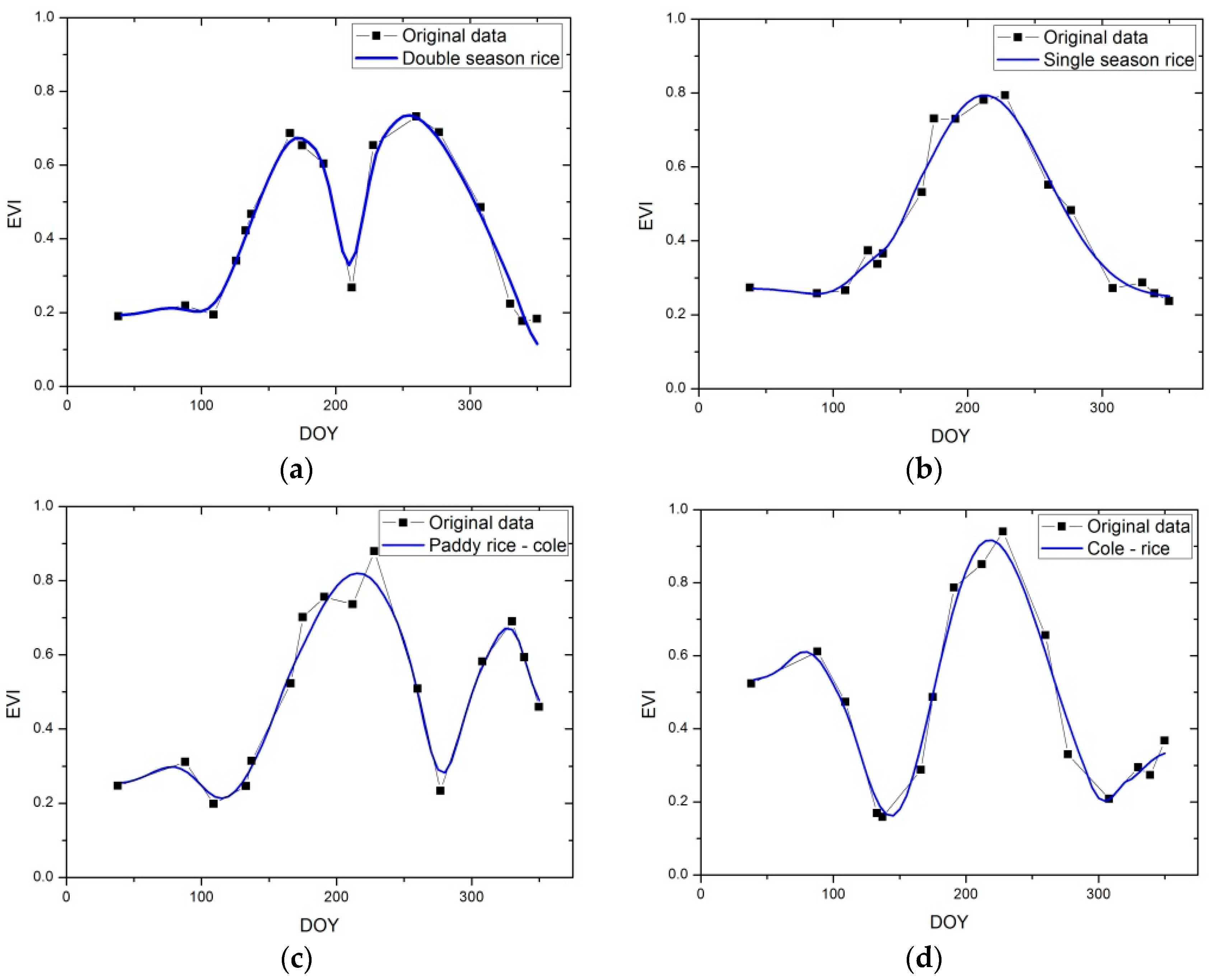
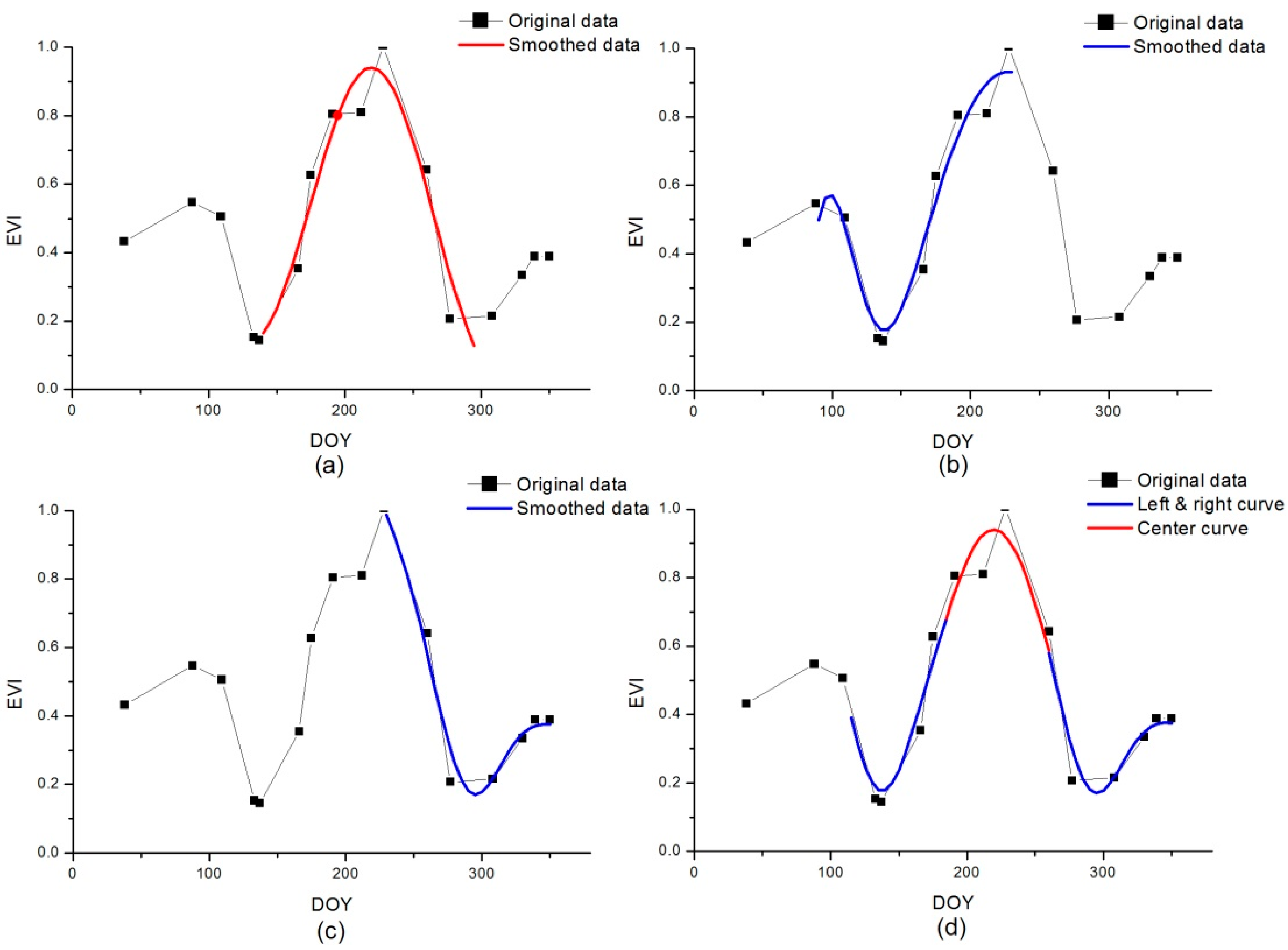
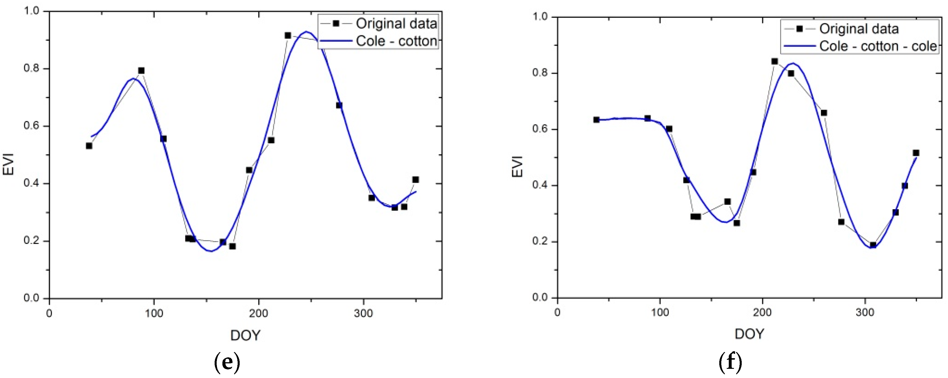
Furthermore, based on temporal segments, the Gaussian and Polynomial fitting methods were used to smooth the local EVI time profile (Equation (1)), from tL to tR. Figure 5a shows the original data and its fitting result (fcenter) between two bottom points (tL and tR). The Gaussian and Polynomial fitting methods were also conducted between every two neighboring summit points. The original data and their fitted functions are shown in Figure 5b,c. To connect fitted local functions, the function fitting method (Equation (2)) was developed, as shown in Figure 5d.
f ( t ) = a e z 2 2 + d t 2 + e + f , where   z = t b c
{ f left t L < t < t L + t C 2 f center t L + t C 2 < t < t R + t c 2 f right t R + t c 2 < t < t R

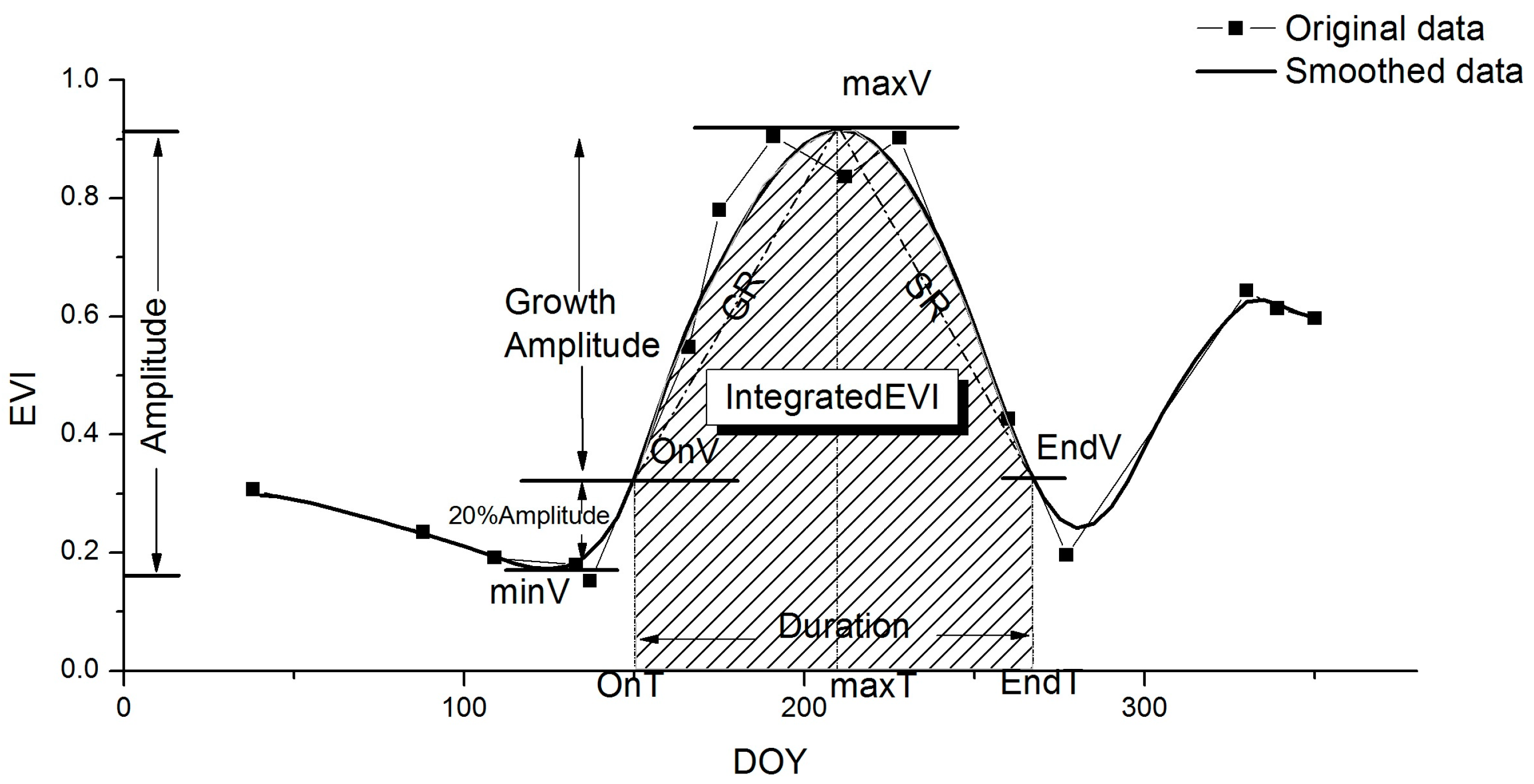
2.3.5. Calculation of EVI Time-Series Metrics

Before the calculation of phenological metrics, the smoothed-and-connected global EVI time profile was disintegrated into temporal parts to recognize crop rotation. Crop rotation reflects the utilization of land use [26]. In our present study, the temporal segments with a fluctuation amplitude greater than 0.2 were considered to be the growth seasons. Then, 11 phenological metrics were derived from the segmented EVI time profile, including the time of onset of greenness (OnT), value at OnT (OnV), time of maximum EVI (maxT), value at maxT (maxV), time of end of greenness (EndT), value at EndT (EndV), growth rate (GR), senescence rate (SR), duration of greenness (DT), integrated area under segmented EVI time profile (IntegratedEVI), and the amplitude of EVI through greenness (Growth Amplitude, or GA). Many of the metrics were adapted from previous studies ([1,27]). Figure 6 shows the derivation of these metrics. The principle task of metric extraction is the identification of OnT and EndT. Their calculation used a threshold strategy, in which the threshold was assigned as an EVI value greater than the bottom value by 20% of the amplitude. Such a threshold value signified the soil background level. The times of the beginning and end of vegetative activity were then acquired, according to the mapping relationship between the threshold and the time axis. GR was estimated from the ratio of amplitude and duration time from beginning to maximum, and similarly, SR was defined. The integrated EVI indicated overall conditions through the growth season, and some studies demonstrated that cumulated indices had a good correlation with potential biomass [28].

2.3.6. Crop Identification Using Random Forest

According to empirical knowledge, typical staple crops in the study area could be planted no more than three times in four seasons of the year. We assumed that crop planting activities occurred three times per field plot. After the global EVI time profile was divided into segmented parts, the 11 phenological metrics of each part were derived. The global time profile that represented the phenological changes throughout the year contained 33 metrics at most. The phenological index of the field, which was rotated less than three times, was set as −1.
In addition to phenological characteristics, spectral information was also of great importance for crop identification. The monthly average reflectance of visible and near infrared bands was utilized to expand the feature set. Moreover, the monthly average EVI and monthly average Normalized Difference Water Index (NDWI) [29] were also combined into the feature set.
With large numbers of accessible features, RF was used to identify crops in the study. RF uses bagging integration, based on a Decision Tree (DT), and introduces a random feature selection process [30]. RF draws bootstrap samples from the original dataset to construct several individual DTs, and the bootstrap process makes it relatively difficult to over-fit. DT randomly selects a subset of variables and chooses the best-splitting variable as the splitting node. This step repeats until the individual DT ends. RF integrates a great many of the abovementioned DTs and finally generates classification results from the majority of the votes. In this study, the feature set was expanded to 105 dimensions, and the RF classifier method was considered to be an ideal choice, because it is easy to implement and has a low computational cost.

3. Results

This analysis was performed on agricultural fields in Lixian, and more than 590,000 field plots were classified. Multi-source medium-resolution images were organized in an orderly way and were transformed into EVI time-series for each field plot. The phenological metrics were derived, and the crop types were recognized. There were three dominant crops: paddy rice (Oryza sativa), cotton (Gossypium hirsutum) and cole (rapeseed). Figure 7 shows the EVI time profiles for those crops in the study area, during 2016. However, the crop planting patterns were varied, due to farming habits or production demands. This part of the paper shows how this method worked in Lixian.

3.1. Time Profile Smoothing

The common agricultural farming patterns are displayed in Figure 8. The following figures depict smoothed EVI time profiles and original data. The smoothed global functions are tightly aligned with the original EVI time-series and preserve vegetative activities that should be retained. The piecewise fitting method showed satisfactory performance for smoothing these kinds of EVI time profiles of complex planting patterns.

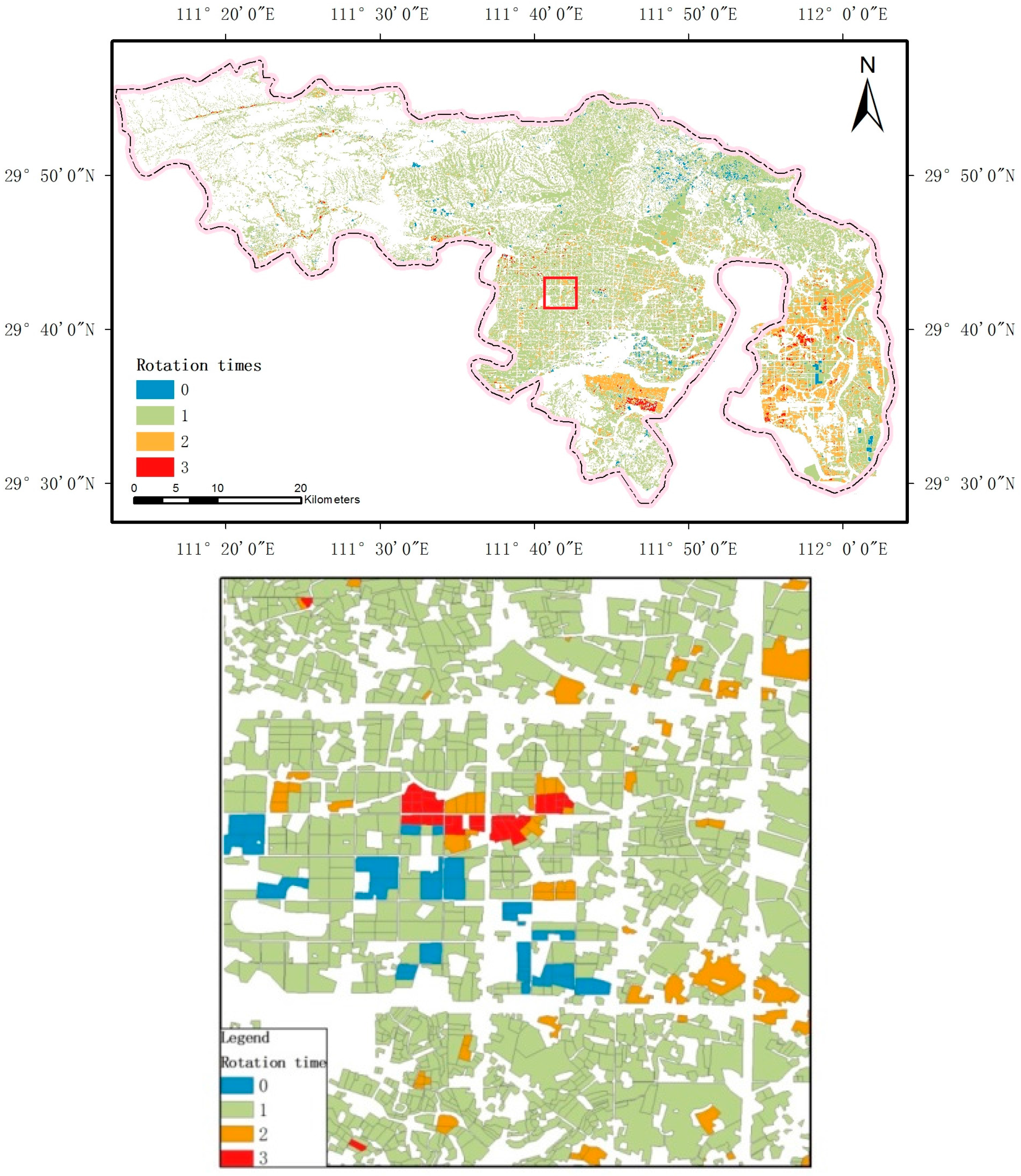
3.2. Rotation Frequency Judgement

By means of the rotation judgement technique, the rotation frequency of all field plots could be recognized. Figure 9 shows the spatial distribution and indicates that most farming fields were planted only once throughout the year, the planting structure of which was simple. They were spatially distributed across the entire area. Approximately 16.39% of the 59,000 plots were rotated, most of which were distributed in the east part of Lixian. This phenomenon can be explained by the natural terrain and climatic conditions. Eastern Lixian is located in the Dongting Lake Plain, which has an average elevation of less than 50 m. Rivers run through the plain, making it convenient for agricultural irrigation. However, the north part of Lixian is mountainous. Agricultural fields are scattered, and the majority of them are planted without rotation.

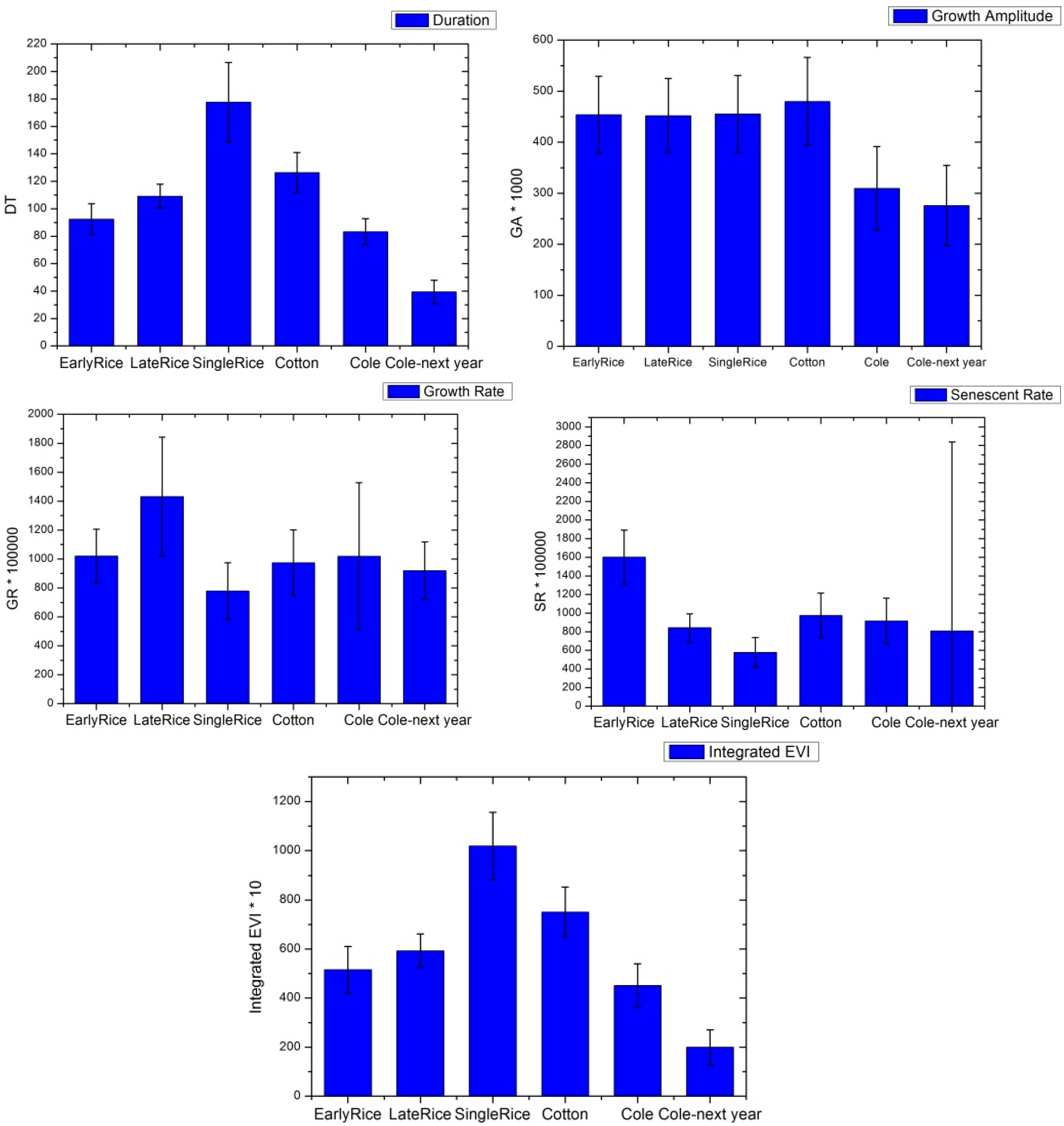
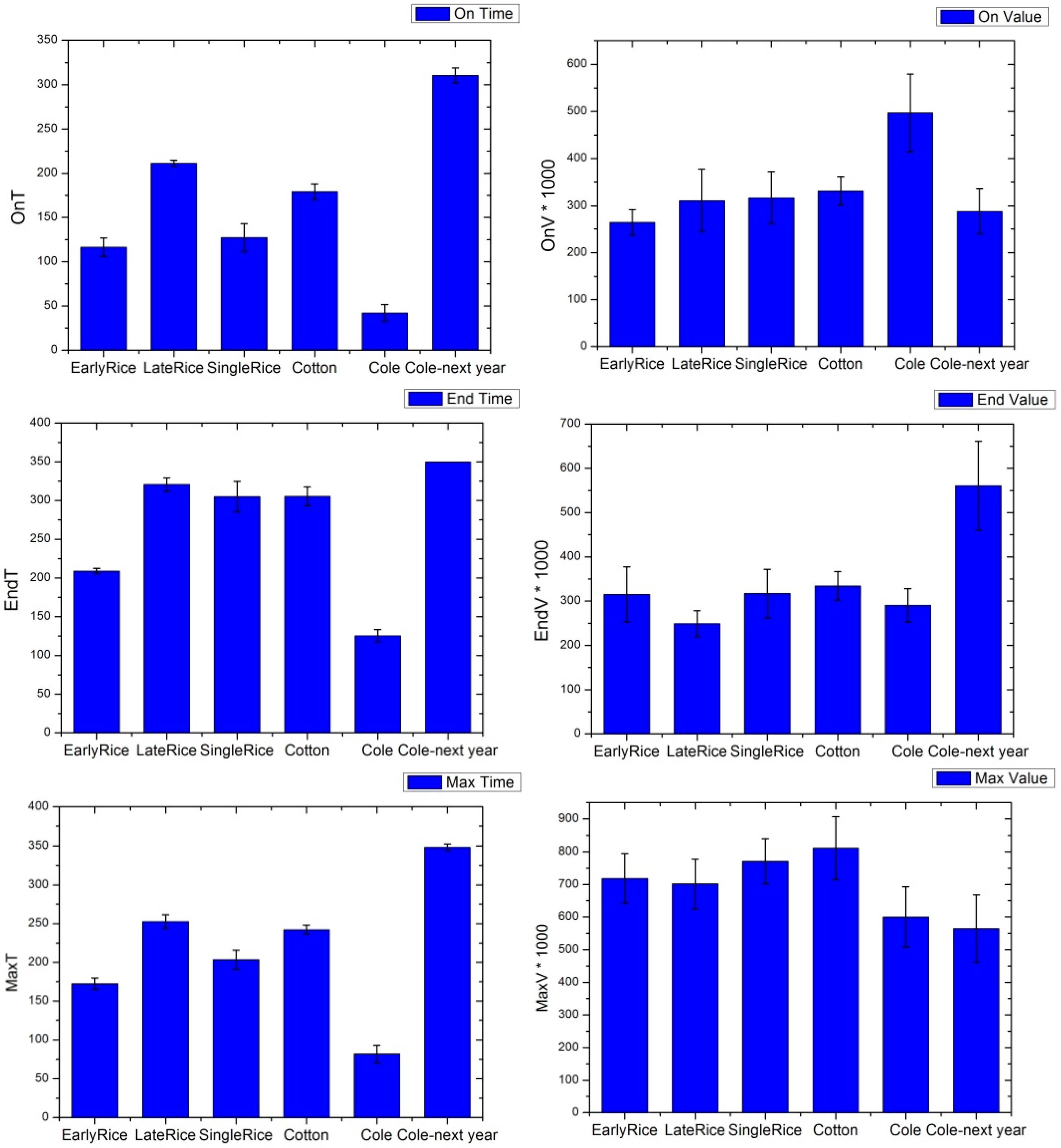
3.3. Phenological Features Extraction

We studied the phenological characteristics of typical crops. According to regular planting patterns, paddy rice that is planted once in a year is called single season rice, and rice that is planted twice is called double season rice. The greenness of single season rice usually lasts from May to October. The cultivation of double season rice is stricter. Transplanted in mid-April, the first season rice (early rice) is harvested in mid-July, and the second season rice (late rice) is planted soon after, to be harvested in late October. The cotton greenness lasts from May to October, and it has five growth stages: sowing, seedling, budding, flower blooming and boll opening periods. In the autumn sowing season, cole is transplanted in late October, then it hibernates through the cold winter weather, and turns green in February of the next year to be harvested in mid-May.
In our study, phenological metrics were derived after the smoothing procedure for the EVI time profiles. Figure 10 shows the statistics of the 11 phenological metrics in the form of bar charts with error bars. In the following charts, the averages and standard deviations describe the given variables. As shown by these charts, phenological characteristics that were related to time (e.g., OnT, EndT, MaxT, DT and integrated EVI) had higher distinguishability than others, because they had more distinct ranges with shorter error bars (especially OnT, EndT and MaxT). Phenological metrics, such as OnV, EndV, MaxV, GR and SR, did not make an obvious distinction for specific crops, as they had similar values between the different crops, and the ranges were broad.

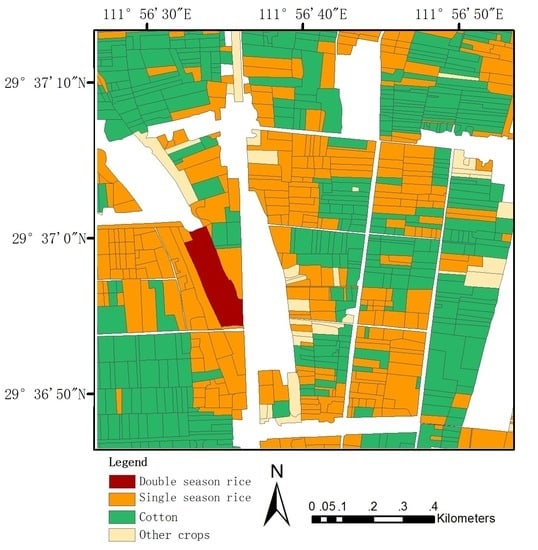
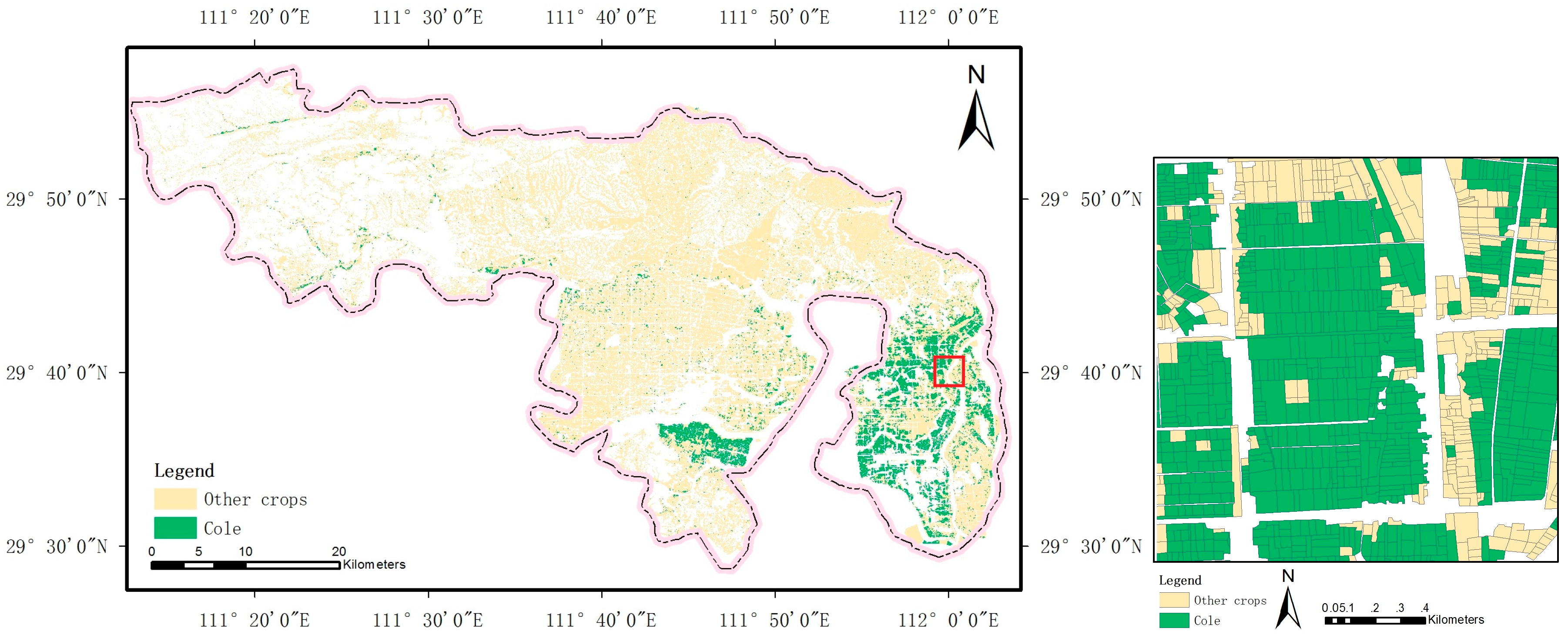
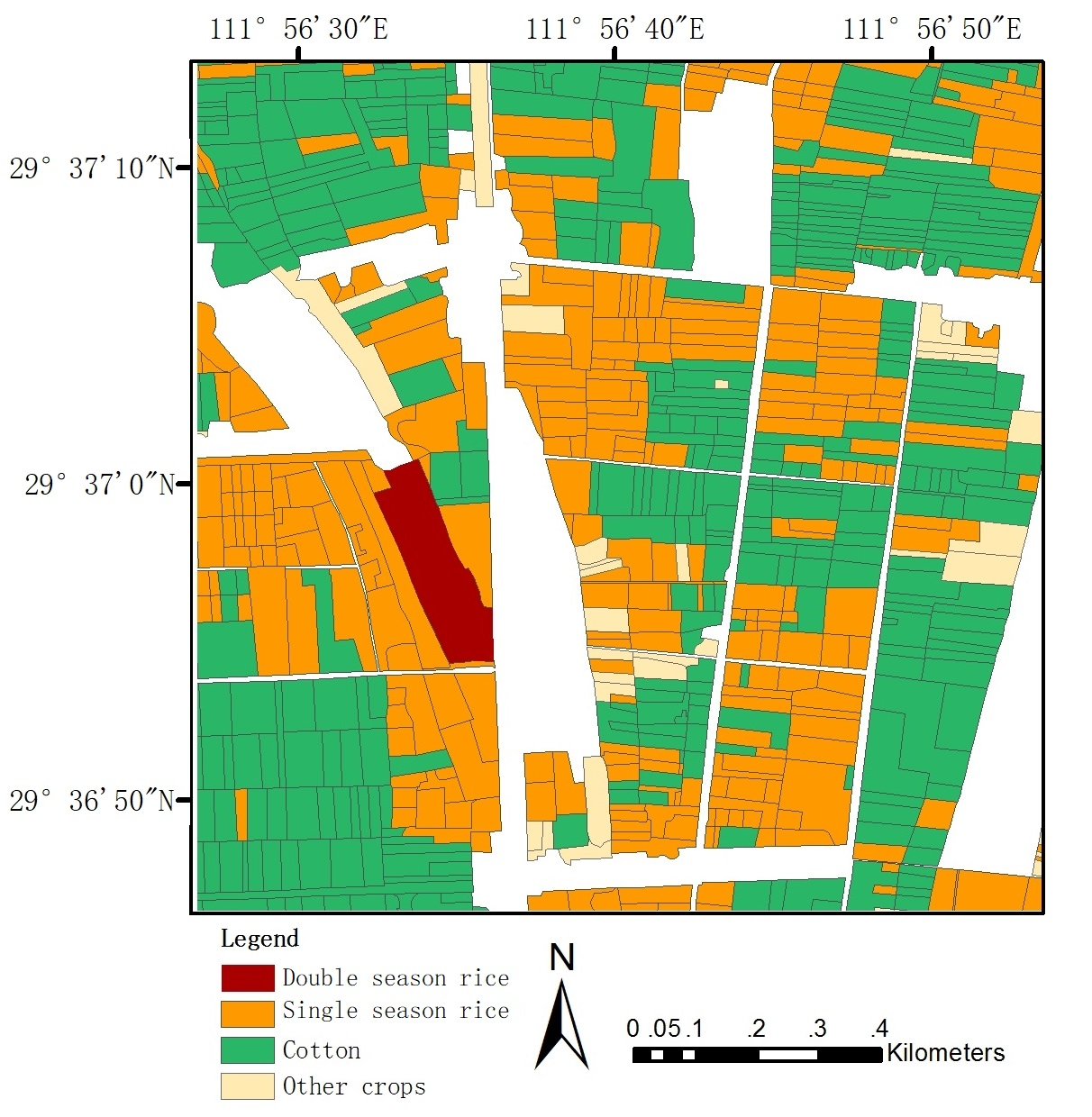
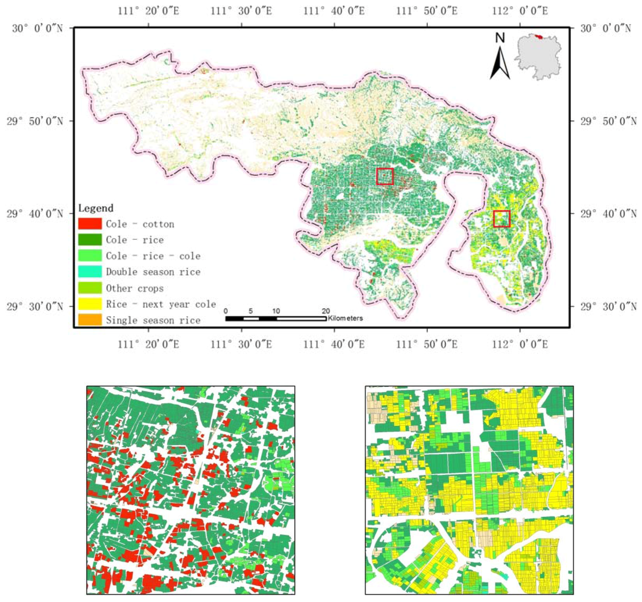
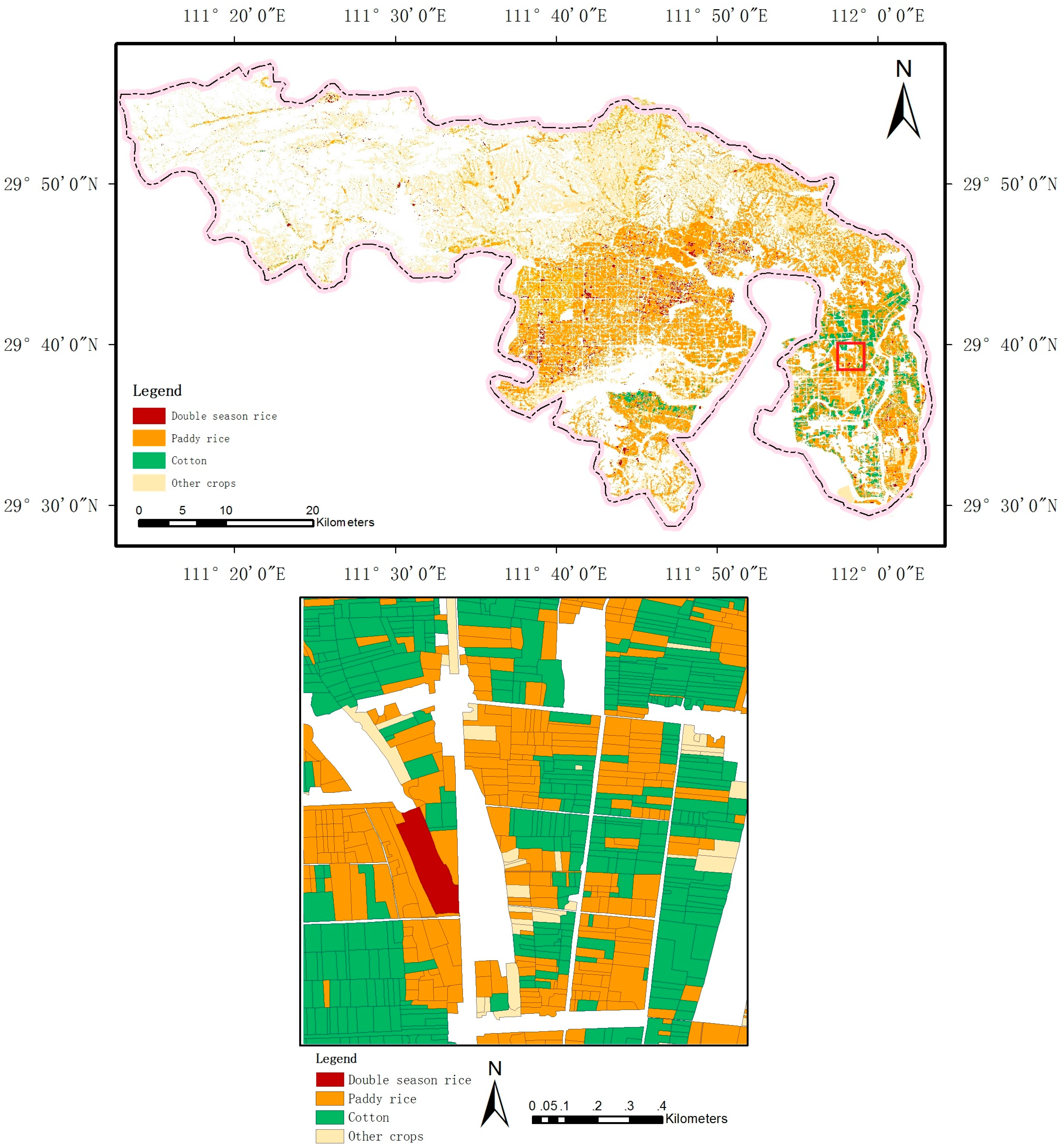
3.4. Crop Classification and Spatial Distribution

By using the RF classifier, more than 590,000 agricultural plots were classified into seven farming types, which were single season paddy rice, paddy rice-cole, cole-paddy rice, double season rice, paddy rice-cotton, cole-paddy rice-cole, and other crops. The ‘-’ indicates crop rotation in sequenced seasons.
The integration of EVI time profile features and multi-temporal spectral features led to a satisfactory performance, the overall accuracy of which was 93.27% (Table 3). Additionally, it indicated that double season rice, cole-paddy rice-cole, and paddy rice-cole could be easily recognized, with accuracies higher than 95%. Single season paddy rice was most likely to be misidentified, due to its simple greenness without regular rotation. The results implied that plots that were rotated multiple times had higher accuracies because agricultural activities usually abided by natural law, and there were more limits on successive planting activities.
The crop spatial distribution was acquired, as shown in Figure 11. The distribution indicated that, in the plains region, farming plots were cultivated adequately for agricultural production. According to classification results, rice occupied the majority of field plots, accounting for approximately 44.32%. There were approximately 46,000 plots that were rotated with single season rice and cole, 11,919 plots were planted with double season rice in 2016, accounting for approximately 2%, and most of them were planted in central Lixian in a scattered distribution. As an autumn-sown crop, cole was likely to be rotated with rice or cotton.
From another perspective, the following figures (Figure 12 and Figure 13) show thematic mappings for specific crop types. Figure 12 displays a map of paddy rice and cotton. Paddy rice includes double season rice, single season rice without rotation, and rice rotated with cole. Cotton was mostly distributed in eastern Lixian, and some was planted in the south. Figure 13 presents a map of autumn-sown cole. Cole was mostly planted in eastern Lixian, with some distributed in the south, and some spread across the study area, even in mountainous terrain.

4. Discussion

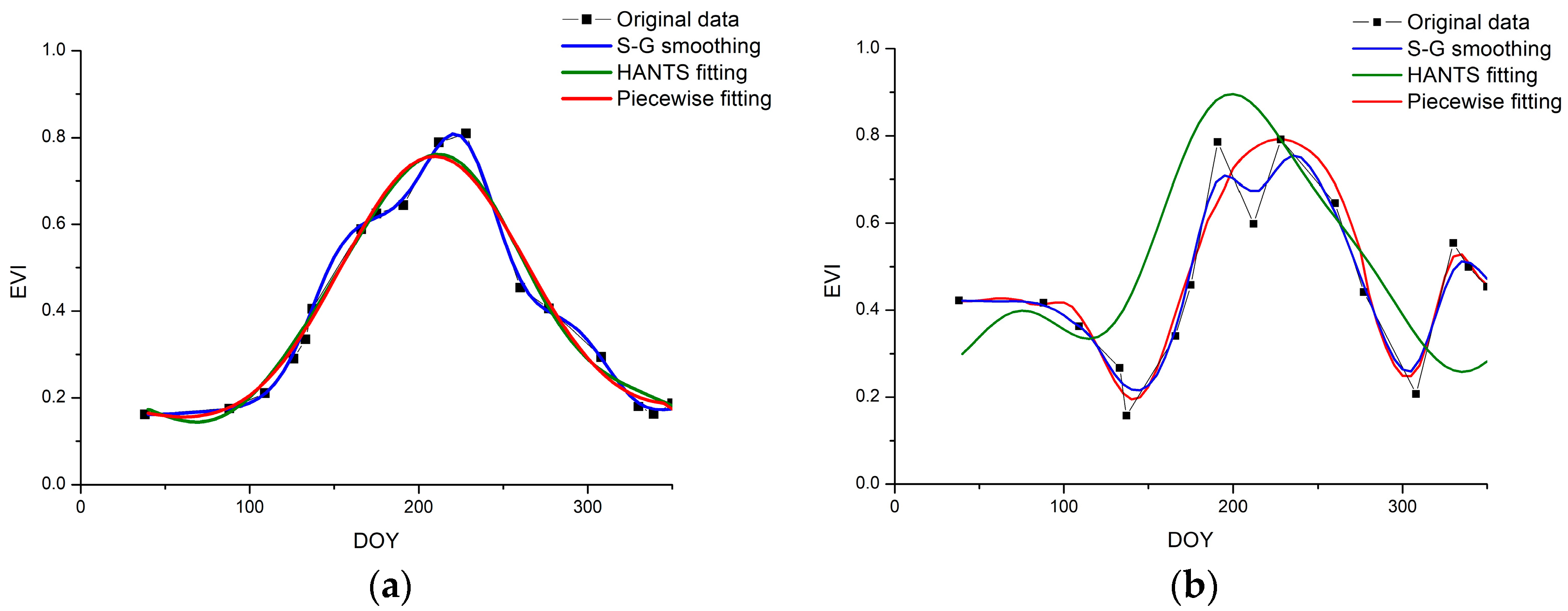
4.1. Comparison of the S–G and HANTS Smoothing Methods

Comparing the S–G and HANTS smoothing method, the results show that the piecewise fitting analysis outperformed the others. Figure 14a shows the EVI time profile of farmland planted with single season rice. The fitting results of the three methods revealed that the HANTS method and our proposed piecewise fitting method were able to fit the temporal curve to a smooth one, whereas S–G conformed tightly to its original shape. To summarize, these methods all work well for fitting an EVI time profile of farmland that is not rotated. Figure 14b shows the EVI time profile with three summits of a rotated farmland. In this figure, the first summit indicates vegetative activity from the beginning of the year, and the third summit shows newly planted crops in autumn. The middle sub-period with the highest peak value indicates a complete growth season. It shows that the effect of the S–G filter was not satisfactory, because it was unable to eliminate unnecessary fluctuations, which causes difficulties in rotation judgement. Another method, the HANTS filter, which fits the time profile using various harmonic functions with different frequencies, can smooth curves, while preserving multiple peaks. However, in regard to time profiles with sub-periods that represent incomplete growth seasons, such as in Figure 14b, it performs poorly. As indicated, it maintains the basic shape of the curve but neglects important partial periods, and the fitted data seriously deviates from the original data. In contrast, our piecewise fitting method can effectively eliminate abnormal fluctuations, which helps to judge crop rotation, and preserves complete or incomplete greenness periods as well.

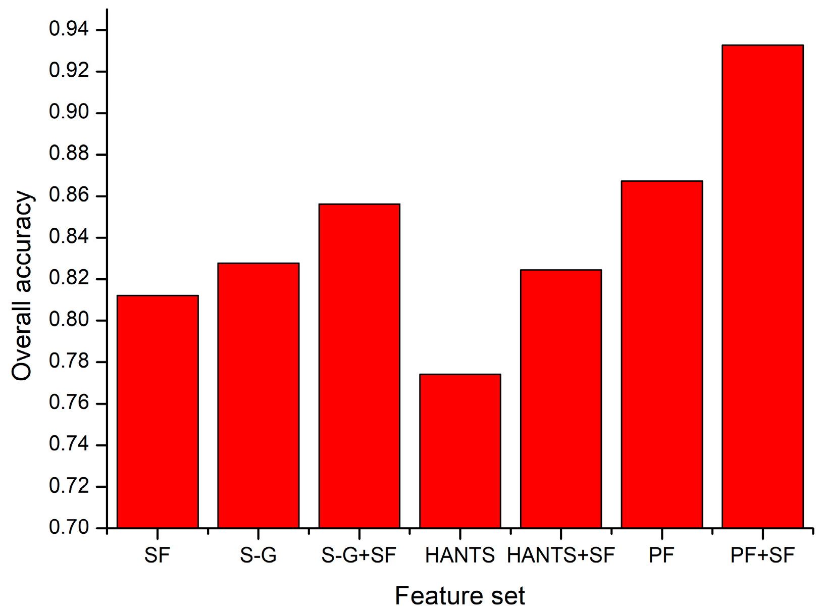
4.2. Classification Accuracy Comparison

Apart from visible distinctions between S–G, HANTS and the piecewise fitting methods in fitting the EVI time profile, the classification accuracy is also improved (Figure 15). We applied three groups of classification experiments using phenological features that were independently derived from the S–G, HANTS and piecewise fitting methods (PF). The overall accuracies were 82.78%, 77.42% and 86.72%, respectively. Phenological metrics of the HANTS fitting method led to the lowest accuracy, whereas the piecewise fitting method had the highest accuracy, but was still below 90%. We performed another three groups of experiments that utilized multi-temporal spectral features (SF) and phenological features, and the accuracies increased by different degrees. The accuracy of S–G + SF (phenological metrics derived from S–G and spectral features) achieved 85.62%, HANTS + SF (phenological metrics derived from HANTS and spectral features) achieved 82.44%, and PF + SF (phenological metrics derived from the piecewise fitting method and spectral features) achieved 93.27%. The results showed that the S–G smoothing method outperformed the HANTS in crop classification, and the piecewise fitting method worked best. Moreover, the integration of SF and phenological metrics significantly improved the classification accuracies.
To analyze the effects of feature set integration, we selected the well-performing piecewise fitting method to compare classifications while using and not using SF. In contrast, the performance of classification using 72 multi-temporal spectral features was unsatisfactory, with an accuracy of 81.21% (Table 4). Without support of phenological features, rotated crops were easily misclassified. For instance, paddy rice-cole was commonly identified as cole-paddy rice-cole, and its accuracy was only 45.61%. In comparison, the accuracy of crop identification using phenological features was better, with an accuracy of 88.73% and kappa coefficient of 0.778 (Table 5). However, without the support of spectral information, the accuracy of cole-paddy rice recognition declined from 90.83% (in Table 3) to 70%, and it was most commonly misclassified as cole-cotton, due to close cultivation times between the rice and cotton.
To summarize, compared with the above results, our study revealed that the integration of methods could significantly improve identification performance (Table 3). Phenological metrics extracted from the EVI time profile reflect vegetative changes during greenness, and multi-temporal spectral information plays an important role when distinguishing specific crops.

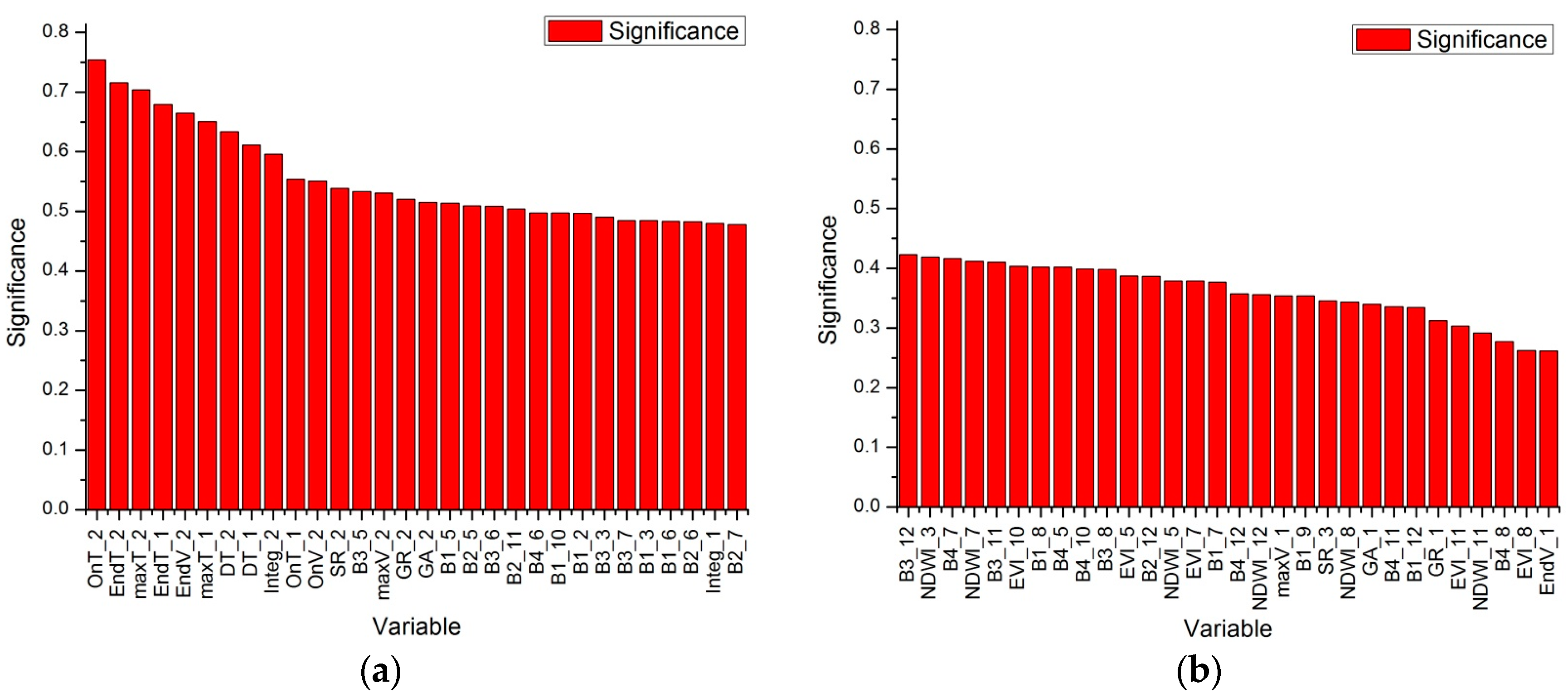
4.3. Features Significance Ranking

The RF classifier generated a significance ranking of the 105 features that were integrated from phenological features and multi-temporal spectral features (Figure 16). In Figure 16, features derived from the EVI time profile were named as ‘OnT_1’, where ‘1’ represented the first greenness. Features extracted from the multi-temporal medium-resolution images were named as ‘B1_3’, where ‘3’ represented blue band reflectance (B1 for blue, B2 for green, B3 for red, and B4 for the NIR band) in March. The results showed that among the feature set, phenological features had great significance for recognizing crops. In the top 20 important features, 15 features were phenological metrics, accounting for a large proportion. Additionally, time-related phenological metrics of field second time greenness made the greatest difference in classification (for instance, OnT_2, EndT_2, MaxT_2 and DT_2).

5. Conclusions

Crop mapping is essential for management of precision agriculture. There is much previous research regarding crop mapping that uses satellite imagery from a single source. Because of the spatial and temporal resolution constraints that are limited by single source satellite sensor performance, problems exist in mixed pixels or salt-and-pepper noise. Based on this issue, our study focused on identifying geo-parcel based crop types by collectively using high spatial and temporal resolution images.
We acquired field plot boundaries from fine-resolution images from GF-2 and constructed EVI time profiles, using medium-resolution images from Landsat 8 OLI and GF-1 WFV sensors. Considering that an analysis of time-series requires high consistency in geometric and radiometric features, we did much pre-processing work of data. Then, multi-temporal spectral information of medium-resolution images was assigned to farming plots. To smooth irregular EVI time-series, we presented a piecewise EVI time profile smoothing method to meet the requirements of rotated farming plots. This could effectively eliminate abnormal fluctuations, which helped with judgement of crop rotation and preserved greenness periods. Following that, the Random Forest classifier was used for crop type identification by integrating phenological metrics that were derived from the smoothed EVI time profile with multi-temporal spectral features, which produced satisfactory accuracies. We demonstrated the significance of phenological features in crop recognition.
In comparison with the S–G and HANTS smoothing methods, the three methods performed well in smoothing the EVI time profile of cultivated land without rotation. When smoothing rotated farmland, the proposed piecewise smoothing method maintained the basic shape of the curve while retaining greenness periods. However, S–G and HANTS behaved unsatisfactorily. The comparison of classification accuracies demonstrated that the S–G smoothing method outperformed the HANTS method in crop classification, and the piecewise fitting method worked best. Additionally, the integration of SF and phenological metrics improved the classification accuracies significantly. So, PF + SF led to the highest classification accuracy.
The limitations of this method mainly exist in the following two aspects. On one hand, for tiny and fragmented plots, the assignment of pixels from medium-resolution images to farmland objects could affect temporal spectral values. This had effects on the EVI time-series and spectral indices, which would eventually impact the classification accuracy to some extent. On the other hand, the threshold of segmenting the global time profile into local parts and judging rotation activity might be optimized in specific situations. These issues will be studied in our future work.

Acknowledgments

This work was supported by the National Key Research and Development Program of China (Grant No. 2017YFB0503600) and the National Natural Science Foundation of China (Grant No. 41631179 and 41601437). The authors appreciate the China Center for Resources Satellite Data and Application and the United States Geological Survey for providing satellite imagery. We are thankful to Hunan Normal University for field surveys and offering the agricultural plot data.

Author Contributions

Yang Yingpin proposed the research methodology, designed and performed the experiments, and wrote the manuscript. Huang Qiting put forwards the basic idea of integration of multi-source data and revised the manuscript. Wu Wei helped to design the experiment and validated experiment accuracy. Luo JianCheng outlined the research topic and assisted with manuscript writing. Gao Lijing, Dong Wen, Wu Tianjun and Hu Xiaodong had great contributions to data preparation and analysis.

Conflicts of Interest

The authors declare no conflict of interest.

References

  1. Reed, B.C.; Brown, J.F.; Vanderzee, D.; Loveland, T.R.; Merchant, J.W.; Ohlen, D.O. Measuring phenological variability from satellite imagery. J. Veg. Sci. 1994, 5, 703–714. [Google Scholar] [CrossRef]
  2. Hill, M.J.; Donald, G.E. Estimating spatio-temporal patterns of agricultural productivity in fragmented landscapes using AVHRR NDVI time series. Remote Sens. Environ. 2003, 84, 367–384. [Google Scholar] [CrossRef]
  3. Sibanda, M.; Murwira, A. The use of multi-temporal MODIS images with ground data to distinguish cotton from maize and sorghum fields in smallholder agricultural landscapes of southern Africa. Int. J. Remote Sens. 2012, 33, 4841–4855. [Google Scholar] [CrossRef]
  4. Viovy, N.; Arino, O.; Belward, A.S. The Best Index Slope Extraction (BISE): A method for reducing noise in NDVI time-series. Int. J. Remote Sens. 1992, 13, 1585–1590. [Google Scholar] [CrossRef]
  5. Ma, M.; Veroustraete, F. Reconstructing pathfinder AVHRR land NDVI time-series data for the northwest of China. Adv. Space Res. 2006, 37, 835–840. [Google Scholar] [CrossRef]
  6. Chen, J.; Jönsson, P.; Tamura, M.; Gu, Z.; Matsushita, B.; Eklundh, L. A simple method for reconstructing a high-quality NDVI time-series data set based on the Savitzky–Golay filter. Remote Sens. Environ. 2004, 91, 332–344. [Google Scholar] [CrossRef]
  7. Jonsson, P.; Eklundh, L. Seasonality extraction by function fitting to time-series of satellite sensor data. Geosci. Remote Sens. IEEE Trans. 2002, 40, 1824–1832. [Google Scholar] [CrossRef]
  8. Atzberger, C.; Eilers, P.C. Evaluating the effectiveness of smoothing algorithms in the absence of ground reference measurements. Int. J. Remote Sens. 2011, 32, 3689–3709. [Google Scholar] [CrossRef]
  9. Zhang, X.; Friedl, M.A.; Schaaf, C.B.; Strahler, A.H.; Hodges, J.C.F.; Gao, F.; Reed, B.C.; Huete, A. Monitoring vegetation phenology using MODIS. Remote Sens. Environ. 2003, 84, 471–475. [Google Scholar] [CrossRef]
  10. Hird, J.N.; Mcdermid, G.J. Noise reduction of NDVI time series: An empirical comparison of selected techniques. Remote Sens. Environ. 2009, 113, 248–258. [Google Scholar] [CrossRef]
  11. Turker, M.; Ozdarici, A. Field-based crop classification using SPOT4, SPOT5, IKONOS and QuickBird imagery for agricultural areas: A comparison study. Int. J. Remote Sens. 2011, 32, 9735–9768. [Google Scholar] [CrossRef]
  12. Immitzer, M.; Atzberger, C.; Koukal, T. Tree species classification with random forest using very high spatial resolution 8-band WordView-2 satellite data. Remote Sens. 2012, 4, 2661–2693. [Google Scholar] [CrossRef]
  13. Yu, Q.; Gong, P.; Clinton, N.; Biging, G.; Kelly, M.; Schirokauer, D. Object-based detailed vegetation classification with airborne high spatial resolution remote sensing imagery. Photogramm. Eng. Remote Sens. 2006, 72, 799–811. [Google Scholar] [CrossRef]
  14. Gao, F.; Masek, J.; Schwaller, M.; Hall, F. On the blending of the Landsat and MODIS surface reflectance: Predicting daily Landsat surface reflectance. IEEE Trans. Geosci. Remote Sens. 2006, 44, 2207–2218. [Google Scholar]
  15. Hilker, T.; Wulder, M.A.; Coops, N.C.; Seitz, N.; White, J.C.; Gao, F.; Masek, J.G.; Stenhouse, G. Generation of dense time series synthetic Landsat data through data blending with MODIS using a spatial and temporal adaptive reflectance fusion model. Remote Sens. Environ. 2009, 113, 1988–1999. [Google Scholar] [CrossRef]
  16. Xie, D.; Zhang, J.; Zhu, X.; Pan, Y.; Liu, H.; Yuan, Z.; Yun, Y. An improved STARFM with help of an Unmixing-based method to generate high spatial and temporal resolution remote sensing data in complex heterogeneous regions. Sensors 2016, 16, 207. [Google Scholar] [CrossRef] [PubMed]
  17. Conrad, C.; Fritsch, S.; Zeidler, J.; Rücker, G.; Dech, S. Per-field irrigated crop classification in arid Central Asia using SPOT and ASTER data. Remote Sens. 2010, 2, 1035–1056. [Google Scholar] [CrossRef] [Green Version]
  18. Singha, M.; Wu, B.; Zhang, M. Object-based paddy rice mapping using HJ-1A/B data and temporal features extracted from time series MODIS NDVI data. Sensors 2016, 17, 10. [Google Scholar] [CrossRef] [PubMed]
  19. Huang, Q.; Qin, Z.; Zeng, Z. A study on the relative radiometric normalization of multi-sources and multi-temporal remote sensing data. J. Geo-Inf. Sci. 2016, 18, 606–614. [Google Scholar]
  20. Wardlow, B.D.; Egbert, S.L.; Kastens, J.H. Analysis of time-series MODIS 250m vegetation index data for crop classification in the U.S. Central great plains. Remote Sens. Environ. 2007, 108, 290–310. [Google Scholar] [CrossRef]
  21. North, H.C.; Pairman, D.; Belliss, S.E.; Mcneill, S.J. Spectral classification of crop groups for land use identification with temporally sparse time-series satellite images. In Proceedings of the IEEE International Geoscience and Remote Sensing Symposium, Melbourne, Australia, 21–26 July 2013; pp. 4237–4240. [Google Scholar]
  22. Demir, B.; Bovolo, F.; Bruzzone, L. Updating land-cover maps by classification of image time series: A novel change-detection-driven transfer learning approach. IEEE Trans. Geosci. Remote Sens. 2013, 51, 300–312. [Google Scholar] [CrossRef]
  23. Hongjun, L.I.; Zheng, L.; Lei, Y.; Chunqiang, L.I.; Zhou, K. Comparison of NDVI and EVI based on EOS/MODIS data. Prog. Geogr. 2007, 26, 26–32. [Google Scholar]
  24. Jönsson, P.; Eklundh, L. Timesat—A program for analyzing time-series of satellite sensor data. Comput. Geosci. 2004, 30, 833–845. [Google Scholar] [CrossRef]
  25. Atkinson, P.M.; Jeganathan, C.; Dash, J.; Atzberger, C. Inter-comparison of four models for smoothing satellite sensor time-series data to estimate vegetation phenology. Remote Sens. Environ. 2012, 123, 400–417. [Google Scholar] [CrossRef]
  26. Fan, C.; Zheng, B.; Myint, S.W.; Aggarwal, R. Characterizing changes in cropping patterns using sequential Landsat imagery: An adaptive threshold approach and application to Phoenix, Arizona. Int. J. Remote Sens. 2014, 35, 7263–7278. [Google Scholar] [CrossRef]
  27. Huang, Q.; Qin, Z.; Zeng, Z. Study on the crop classification and planting area estimation at land parcel scale using multisources satellite data. J. Geo-Inf. Sci. 2016, 18, 708–717. [Google Scholar]
  28. Tucker, C.J.; Elgin, J.H.; McMurtrey, J.E.; Fan, C.J. Monitoring corn and soybean crop development with hand-held radiometer spectral data. Remote Sens. Environ. 1979, 8, 237–248. [Google Scholar] [CrossRef]
  29. Hao, P.; Zhan, Y.; Wang, L.; Niu, Z.; Shakir, M. Feature selection of time series MODIS data for early crop classification using random forest: A case study in Kansas, USA. Remote Sens. 2015, 7, 5347–5369. [Google Scholar] [CrossRef]
  30. Breiman, L. Random forest. Mach. Learn. 2001, 45, 5–32. [Google Scholar] [CrossRef]
Figure 1. The location of the study area and an image of the sub-area, for detail.
Remotesensing 09 01298 g001
Figure 2. The main steps of using fine-resolution and medium-resolution imagery to classify crops (VIS/NIR (visible and near infrared)).
Remotesensing 09 01298 g002
Figure 3. The precise boundaries of agricultural farming plots.
Remotesensing 09 01298 g003
Figure 4. Typical patterns of the time profiles for filtered NDVI and EVI. (a) EVI and NDVI time profiles of single season rice; (b) EVI and NDVI time profiles of double season rice.
Remotesensing 09 01298 g004
Figure 5. Piecewise Gaussian and Polynomial smoothing methods.
Remotesensing 09 01298 g005
Figure 6. Calculation of phenological metrics.
Remotesensing 09 01298 g006
Figure 7. EVI time profiles for dominant crops in the study area during 2016 (DOY is day of year).
Remotesensing 09 01298 g007
Figure 8. Typical agricultural farming patterns in Lixian.
Remotesensing 09 01298 g008aRemotesensing 09 01298 g008b
Figure 9. Spatial distribution of crop rotation.
Remotesensing 09 01298 g009
Figure 10. Phenological statistics (‘cole’ represents the cole sown in autumn of the previous year, and ‘cole-next year’ represents cole that was transplanted in one year and is to be harvested in the next year).
Remotesensing 09 01298 g010aRemotesensing 09 01298 g010b
Figure 11. Field-based crop type identification.
Remotesensing 09 01298 g011
Figure 12. Map of double season rice, paddy rice and cotton (paddy rice includes single season rice and rice rotated with cole).
Remotesensing 09 01298 g012
Figure 13. Map of cole.
Remotesensing 09 01298 g013
Figure 14. Comparisons between the Savitzky–Golay Filter (S–G) smoothing method, the HANTS fitting method and our piecewise fitting method. (a) The EVI time profile of single season rice farmland; (b) The EVI time profile of a “cole-paddy rice-cole” rotated farmland.
Remotesensing 09 01298 g014
Figure 15. Overall accuracy comparison between classifications using different feature sets. SF means spectral features, PF means the proposed piecewise fitting method.
Remotesensing 09 01298 g015
Figure 16. (a) The top 30 significant features; (b) The last 30 significant features.
Remotesensing 09 01298 g016
Table 1. Technical specifications of the GF-1 WFV sensors.
SatellitePayloadsBands No.Spectral Range (μm)Spatial Resolution (m)Swath Width (km)Repetition Cycle (Day)
GF-1WFV10.45–0.5216800 (four cameras combined)4
20.52–0.59
30.63–0.69
40.77–0.89
Table 2. Information for the medium-resolution images that were used in the study (WFV1 for NO.1 WFV sensor in GF-1, and so on).
SatelliteSensorAcquisition TimeDay of Year
GF-1WFV28-02-201638
GF-1WFV128-03-201688
GF-1WFV318-04-2016109
GF-1WFV405-05-2016126
GF-1WFV112-05-2016133
GF-1WFV116-05-2016137
GF-1WFV214-06-2016166
GF-1WFV114-06-2016166
GF-1WFV423-06-2016175
GF-1WFV209-07-2016191
GF-1WFV309-07-2016191
GF-1WFV125-07-2016207
GF-1WFV129-07-2016211
GF-1WFV315-08-2016228
GF-1WFV303-10-2016277
GF-1WFV104-11-2016308
GF-1WFV426-11-2016330
GF-1WFV404-12-2016339
GF-1WFV115-12-2016350
Landsat 8OLI30-07-2016212
Landsat 8OLI16-09-2016260
Table 3. Confusion matrix of classification using phenological features and spectral features.
All FeaturesPaddy RicePaddy Rice-ColeCole-Paddy RiceDouble Season Paddy RiceCole-CottonCole-Paddy Rice-ColeOther CropsUser’s Accuracy
Paddy Rice7900000290.7315
Paddy Rice-Cole0170000100.9942
Cole-Paddy Rice00218021100.9083
Double Season Paddy Rice0011152000.9746
Cole-Cotton00120121000.9098
Cole-Paddy Rice-Cole0000024530.9880
Other Crops3170022020.9395
Overall Accuracy0.9327
Kappa0.9201
Table 4. Confusion matrix of classification using spectral features.
Spectral FeaturesPaddy RicePaddy Rice-ColeCole-Paddy RiceDouble Season Paddy RiceCole-CottonCole-Paddy Rice-ColeOther CropsUser’s Accuracy
Paddy Rice8025001200.7407
Paddy Rice-Cole60782003010.4561
Cole-Paddy Rice100201021800.8375
Double Season Paddy Rice1001140030.9661
Cole-Cotton10130118010.8872
Cole-Paddy Rice-Cole11190422410.8960
Other Crops13180501880.8744
Overall Accuracy0.8121
Kappa0.7777
Table 5. Confusion matrix of classification using phenological features.
Phenological FeaturesPaddy RicePaddy Rice-ColeCole-Paddy RiceDouble Season Paddy RiceCole-CottonCole-Paddy Rice-ColeOther CropsUser’s Accuracy
Paddy Rice1020000060.9444
Paddy Rice-Cole0170000100.9942
Cole-Paddy Rice00168071100.7000
Double Season paddy Rice0001133200.9576
Cole-Cotton00170116000.8722
Cole-Paddy Rice-Cole0000524300.9798
Other Crops23053021820.8465
Overall Accuracy0.8873
Kappa0.8672

