Article

Performance Evaluation of Downscaling Sentinel-2 Imagery for Land Use and Land Cover Classification by Spectral-Spatial Features

1
Key Laboratory for Satellite Mapping Technology and Applications of National Administration of Surveying, Mapping and Geoinformation of China, Nanjing 210023, China
2
Jiangsu Provincial Key Laboratory of Geographic Information Science and Technology, Nanjing University, Nanjing 210023, China
3
Research Center for Advanced Science and Technology, The University of Tokyo, Tokyo 113-8654, Japan
4
School of Resource Engineering, Longyan University, Longyan 364012, China
5
Collaborative Innovation Center for the South China Sea Studies, Nanjing University, Nanjing 210023, China
*
Author to whom correspondence should be addressed.
Remote Sens. 2017, 9(12), 1274; https://doi.org/10.3390/rs9121274
Submission received: 2 November 2017 / Revised: 4 December 2017 / Accepted: 6 December 2017 / Published: 7 December 2017
(This article belongs to the Special Issue Remote Sensing Image Downscaling)

Abstract

:
Land Use and Land Cover (LULC) classification is vital for environmental and ecological applications. Sentinel-2 is a new generation land monitoring satellite with the advantages of novel spectral capabilities, wide coverage and fine spatial and temporal resolutions. The effects of different spatial resolution unification schemes and methods on LULC classification have been scarcely investigated for Sentinel-2. This paper bridged this gap by comparing the differences between upscaling and downscaling as well as different downscaling algorithms from the point of view of LULC classification accuracy. The studied downscaling algorithms include nearest neighbor resampling and five popular pansharpening methods, namely, Gram-Schmidt (GS), nearest neighbor diffusion (NNDiffusion), PANSHARP algorithm proposed by Y. Zhang, wavelet transformation fusion (WTF) and high-pass filter fusion (HPF). Two spatial features, textural metrics derived from Grey-Level-Co-occurrence Matrix (GLCM) and extended attribute profiles (EAPs), are investigated to make up for the shortcoming of pixel-based spectral classification. Random forest (RF) is adopted as the classifier. The experiment was conducted in Xitiaoxi watershed, China. The results demonstrated that downscaling obviously outperforms upscaling in terms of classification accuracy. For downscaling, image sharpening has no obvious advantages than spatial interpolation. Different image sharpening algorithms have distinct effects. Two multiresolution analysis (MRA)-based methods, i.e., WTF and HFP, achieve the best performance. GS achieved a similar accuracy with NNDiffusion and PANSHARP. Compared to image sharpening, the introduction of spatial features, both GLCM and EAPs can greatly improve the classification accuracy for Sentinel-2 imagery. Their effects on overall accuracy are similar but differ significantly to specific classes. In general, using the spectral bands downscaled by nearest neighbor interpolation can meet the requirements of regional LULC applications, and the GLCM and EAPs spatial features can be used to obtain more precise classification maps.

Graphical Abstract

1. Introduction

Land Use and Land Cover (LULC) maps not only describe the composition and distribution of the natural elements on the land surface but also reflect the anthropogenic effects on these elements [1]. Remote sensing perfectly meets the requirements of LULC classification and monitoring due to its robust, consistent, repeatable and cost-effective capacities [2].
Sentinel-2 is a new generation optical satellite for land monitoring developed by European Space Agency for data continuity and enhancement of the Landsat and SPOT missions [3]. It has the combination of high spatial resolution and revisits frequently, novel spectral capabilities, and wide coverage, which offer more advantages over Landsat series in regional LULC classification. However, the existing researches mainly focus on parameter estimation (e.g., vegetation biophysical and water quality [4,5,6]) and specific target detection (e.g., water body, greenhouses, and built-up areas [7,8,9,10]). Vegetation species classification has also attracted great attention with the aim of assessing the potential of its three unique red-edge bands [11,12]. As with MODIS and ASTER, Sentinel-2 has the characteristics of inconsistent spatial resolutions. Then, unifying the spatial resolution of different bands is a prerequisite for many applications. Usually, there are two categories of schemes to execute the geometric unification. One is to upscale the fine resolution bands to match the coarse resolution bands. The other is to downscale the coarse resolution bands to match the fine resolution bands [13]. Choosing which scheme depends on the application purpose. For example, upscaling perfectly meets the requirement of lithologic mapping for ASTER with the ability of complete preservation of the original spatial and spectral information of its short wave infrared (SWIR) bands, which are the characteristic bands of minerals (i.e., clay, carbonates and sulfates) and reduce data volume at the same time [14,15]. However, for LULC classification, downscaling is more suitable due to the capability of fully utilizing the valuable detailed information obtained by fine resolution bands [16].
In the context of remote sensing image processing, upscaling and downscaling are usually implemented by spatial interpolation. Nearest neighbor interpolation is the most popular one because of its straightforward implementation [17,18]. Besides, pansharpening is also commonly used in downscaling [19,20]. Pansharpening can consequently be defined as a pixel-level fusion, which is to merge the geometric details of a high resolution (HR) image into low resolution multispectral (LRMS) bands [21,22]. It increases the spatial information at the cost of a certain degree of spectral information loss, represented by a more or less color distortion [23]. Typical pansharpening techniques include component substitution (CS), statistics, and multiresolution analysis (MRA) based methods. The fusion quality of different algorithms depends on data used and the application purpose [24,25]. For example, the Intensity-Hue-Saturation (IHS) and Principal Components Analysis (PCA) transformation, which are based on CS, can achieve a satisfactory result for visual interpretation on Landsat TM, SPOT, and IRS. However, they are less effective on those data acquired from satellites launched after 1999 because of the PAN band wavelength extended from visible into the near infrared (e.g., IKONOS and QuickBird), or for quantitative analysis [23,26]. As the sensor and application dependence of fusion quality, the effects of different image sharpening algorithms on LULC classification have been investigated using MODIS and ASTER [27,28]. Although there are already several attempts in downscaling the Sentinel-2 data, they tend to focus on the quantitative analysis of fusion quality or its improvement in water extraction and vegetation monitoring, and the effects on LULC classification accuracy of Sentinel-2 are still untested and urgently needed [6,7,29,30,31].
Pansharpening techniques can be adapted to image sharpening of multispectral data (e.g., Sentinel-2) that have multiple spatial resolutions depending on bands and also multiple bands at the highest spatial resolution. The most straightforward way of adapting pansharpening techniques to image sharpening of multiresolution multispectral data is to select one of the highest resolution bands for each LRMS band as a PAN-like band [7,13]. For Sentinel-2 image sharpening, it is always favorable to take advantages of the four 10-m bands and six 20-m bands to provide the richest spatial and spectral information for reliable LULC maps. In other words, the Sentinel-2 sharpening task is to merge the spatial details of its 10-m bands into its 20-m bands and generate an image with all ten multispectral bands at a 10-m spatial resolution.
In order to investigate the impact of spatial resolution unification schemes on LULC classification, we compared the classification accuracy of images generated by one upscaling and six downscaling methods, including nearest neighbor interpolation, which is also used as the spatial interpolation method in upscaling, and five pansharpening algorithms, namely, Gram-Schmidt (GS), nearest neighbor diffusion (NNDiffusion), PANSHARP proposed by Y. Zhang, wavelet transformation fusion (WTF) and high-pass filter fusion (HPF). However, the pixel-based classification only utilized spectral information, without considering texture and contextual information, which has not enough capability to fully evaluate the effects of image sharpening on classification [32,33]. To compensate for this shortcoming, we added spatial features to ensure the assessment was more comprehensive and unbiased. Spatial features can be derived by several approaches; the most widely used are textural analysis and mathematical morphology [34,35]. Texture is an effective representation of spatial relationship and contextual information. Grey-Level-Co-occurrence Matrix (GLCM) has been proved to be of great value in LULC classification on several data [36,37,38,39]. Mathematical morphology is a framework which can be extended into morphological profiles (MPs), extended MPs (EMPs), attribute profiles (APs), extended APs (EAPs), extended multi-AP (EMAP) [40,41,42]. APs provide a multilevel characterization of the input image by the sequential application of morphological attribute filters, and it can be considered as a generalization of MPs. EAPs is computed on a few principal components (PCs) extracted by Principal Components Analysis (PCA) transformation, not only addresses the limitation of MPs in the capability of describing spatial features, but addresses the constraint of APs in the computational intensity and reduce the dimensionality of the original feature space. Thus, EAPs has been widely used to improve the accuracy of LULC classification on high resolution and hyperspectral images [43,44]. Although the EAPs have been successfully applied to middle resolution remote sensing images, they were not investigated in Sentinel-2, as well as GLCM [45,46].
The specific research objectives are to: (1) evaluate the effects of the two different spatial resolution unification schemes, i.e., upscaling and downscaling, on classification accuracy of Sentinel-2 imagery; (2) assess the role of image sharpening techniques in LULC classification; and (3) investigate the value of spatial features, i.e., EAPs and GLCM, in LULC classification. The remainder of this paper is organized as follows: the general situation of study area and data are presented in Section 2. Spatial resolution unification schemes and datasets, as well as the classification system, are introduced in Section 3. Section 4 illustrates and discusses the classification results. Finally, conclusions are drawn in Section 5.

2. Study Area and Data
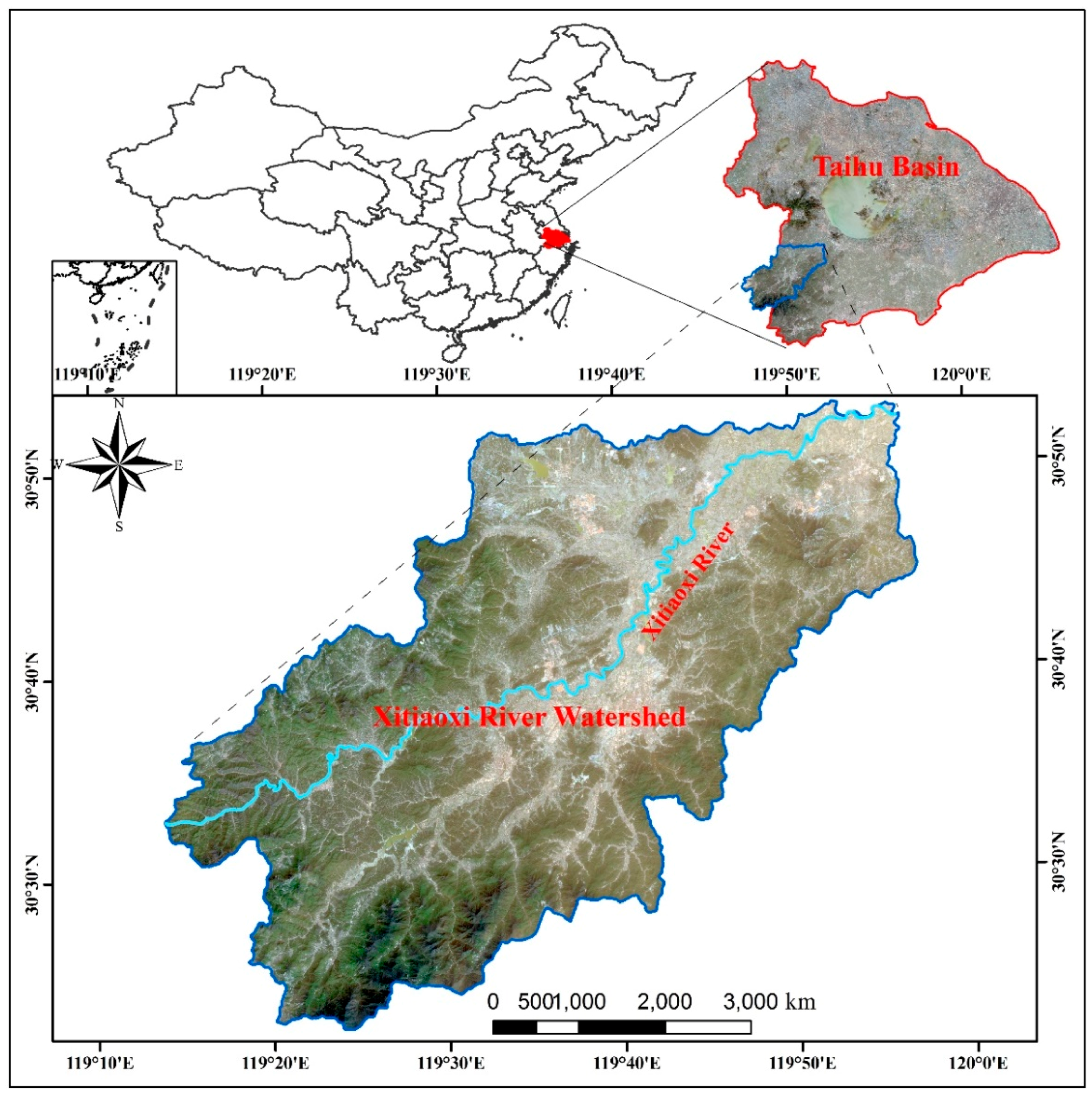
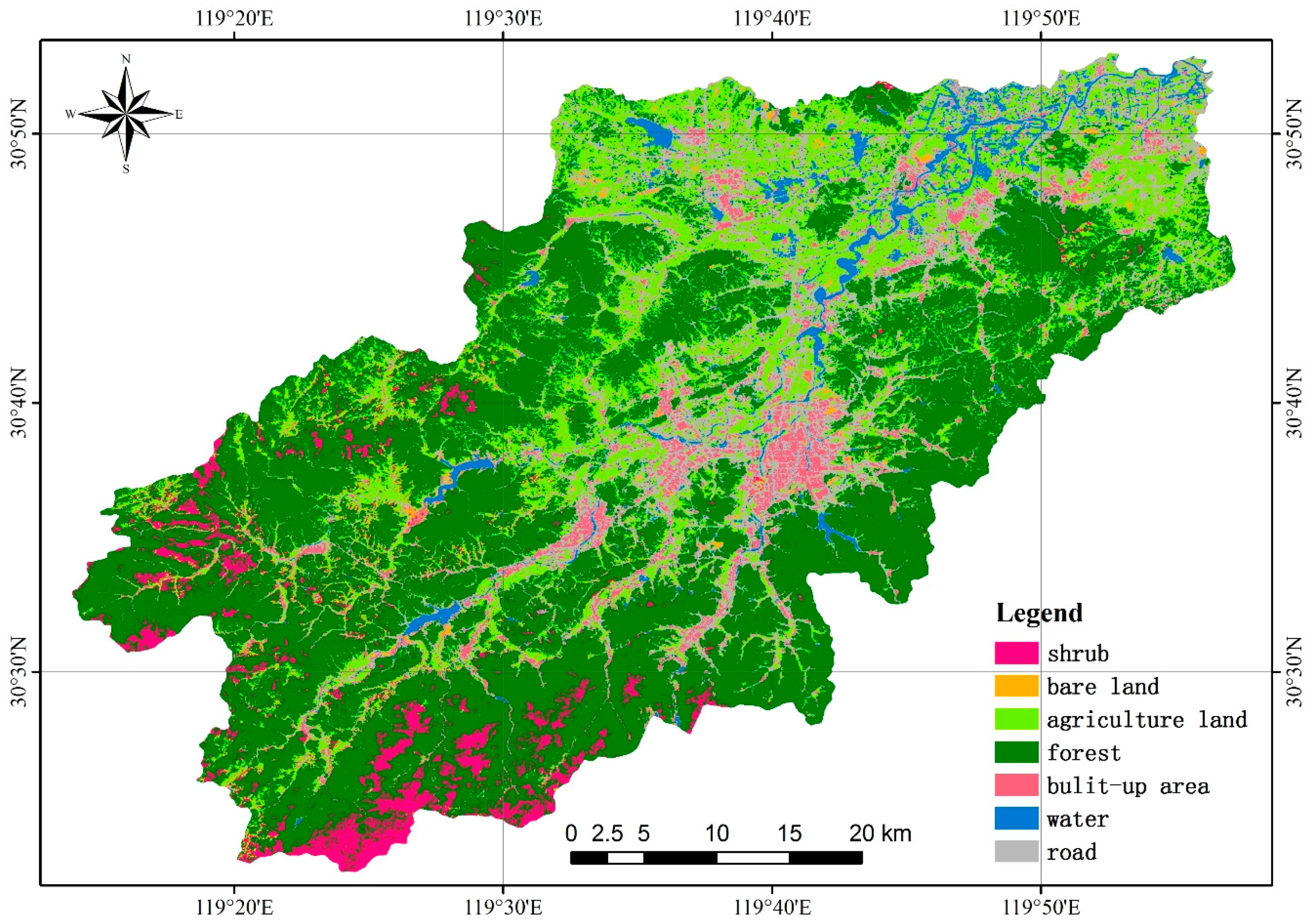
2.1. Study Area

Taihu Lake, the third largest freshwater lake in China, has been encountering the threat of water eutrophication over the last three decades, which was consistent with the rapid urbanization and LULC changes in the basin [47,48]. Xitiaoxi River is the main inflow river in the southwest of the lake, and annually discharges nearly 30% of water volume (its location shown in Figure 1). This river is 159 km long and encompasses a watershed area of 2200 km2 (30°22.5′–30°53′N, 119°14′–119°57′E; its range as shown in Figure 1), accounting for six percent of the entire Taihu Basin. A more detailed LULC map plays a vital role in analyzing rural nonpoint source pollution of this watershed and its effect on water quality to the lake. The watershed belongs to northern subtropical monsoon climate with an average annual temperature of 15.5 °C and a mean annual precipitation of 1465.8 mm. The northeastern part of this basin is flat land with the lowest elevation of 1.2 m, and the southwest is mountainous with the highest elevation of 1587 m [49]. The dominant land use types of this watershed are forest and agricultural land as it located mainly in the rural area.

2.2. Data

Sentinel-2 is a twin satellites constellation consisting of Sentinal-2A launched on 23 June 2015 and Sentinal-2B followed on 7 March 2017. The two satellites flying in the same orbit but phased at 180° to provide a high revisit frequency of five days with a constant view angle to the same target area. The onboard Multispectral Imager Instruments (MSI) covers a field of view of 290 km and provides thirteen spectral bands from visible near-infrared (VNIR) to SWIR, with the ground sampling distance (GSD) of four bands at 10 m, six bands at 20 m and three bands at 60 m [50]. The coastal band (band 1), water vapor band (band 9) and cirrus band (band 10) are at the same GSD of 60 m. Three red edge bands (i.e., bands 5, 6, and 7), an NIR band (band 8a), and two SWIR bands (bands 11 and 12) are the same at 20 m. Bands 2, 3, and 4 are three visible bands (R/G/B) at a 10-m GSD as the left NIR band (band 8). Sentinel-2 standard level-1C (L1C) products are available freely from the Copernicus Scientific Data Hub website as Top-of-Atmosphere (TOA) reflectance ortho-images in terms of elementary granules of fixed size. The granules, also called tiles, are the minimum indivisible partition of a product in 100 × 100 km2 with UTM/WGS84 projection [7]. The whole watershed is over the coverage of one tile, and two tiles acquired on 28 February 2017 with the center position coordinates of 31°6′45′′N, 119°40′20′′E and 30°12′39′′N, 119°38′52′′E, respectively, were used for subsequent processing.

3. Methods

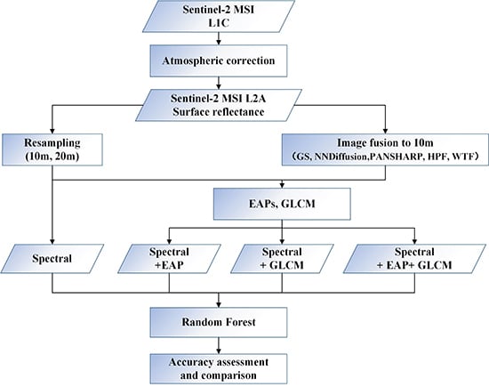
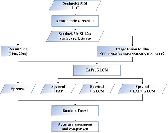
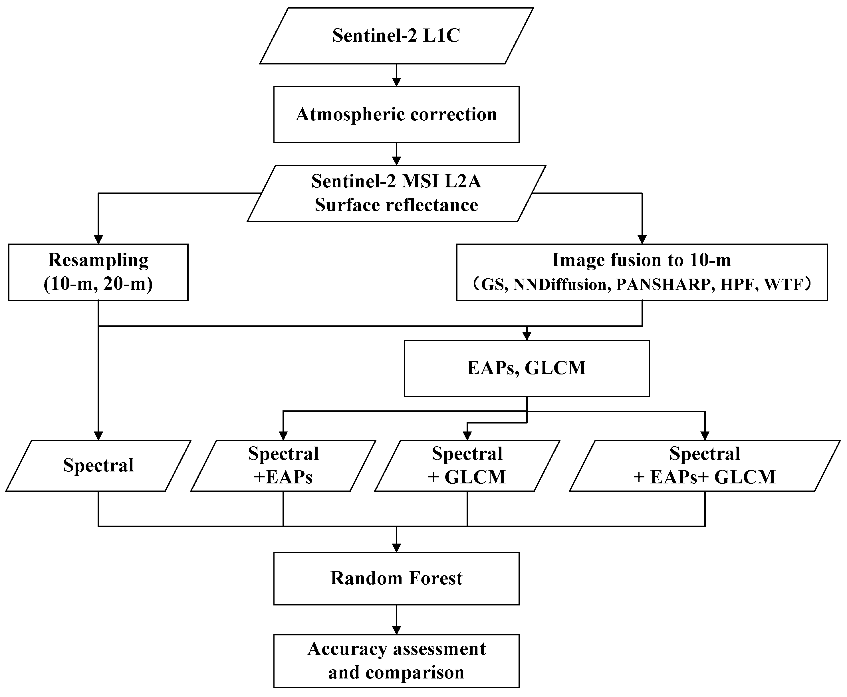
3.1. LUCC Classification Procedure

Figure 2 illustrates a flowchart of the methodology used in this study. In the first stage, the Sentinel-2 L1C product was geometrically unified into seven datasets at two different spatial resolutions. Then, EAPs and GLCM were calculated and integrated with spectral bands separately or together to form four feature sets. Finally, seven data sets with four feature sets generate twenty-eight classification scenarios, each of which was delineated into seven classes, including shrub, forest, agricultural land, bare land, built-up areas, water, and road with random forest.

3.2. Geometric Unification Schemes by Upscaling and Downscaling

In data processing, there is no need to do further geometric correction for L1C products, and only atmospheric correction and spatial resolution unification are required. The atmospheric effects can be well eliminated by the Sen2Cor algorithm [51]. After Sen2Cor processing, the L1C TOA reflectance values were converted into Level-2A (L2A) Bottom-of-Atmosphere (BOA) reflectance values.
The spatial resolution was unified by one upscaling and six downscaling methods. As the most common way in re-scaling the pixel resolutions, nearest neighbor resampling was used both in upscaling and downscaling in our study, and the downscaled image by resampling is regarded as the benchmark. For downscaling, it just divides one pixel into four adjacent pixels with the same value and has the advantages of completely preserving original information, simple and fast [17]. Besides resampling, five popular pansharpening algorithms, namely, GS, NNDiffusion, PANSHARP, WTF, and HPF were used in downscaling.
GS is a representative pansharpening method based on CS. The CS-based methods substitute an HR image for the selected band after spectral transformation. GS replace the HR band (usually refers to PAN band) for the first band of Gram-Schmidt transformation performed by a simulated low resolution (LR) image averaged by the LRMS bands as the first band and followed by these LRMS bands [20].
NNDiffusion and PANSHARP are all based on statistics. They use statistics to decide the contribution of each MS bands to the PAN band [52]. Different from PANSHARP, NNDiffusion decides the weights according to a diffusion model inferred from the Pan band that relates the similarity of the pixel of interest to the neighboring superpixels [53]. The statistics-based algorithms have advantages over traditional CS-based algorithms (e.g., IHS and PCA) in spectral fidelity for those sensors whose PAN band’s wavelength extended into near infrared.
WTF and HPF are traditional image fusion algorithms based on MRA. Both of them extract the high frequency information from HR image and inject to LRMS image; however, their high frequency components extraction methods are distinct. WTF extracts the high frequency information by a wavelet transformation and integrated with every LRMS bands by replacing the low frequency approximation generated from wavelet transformation with the LRMS image and followed by an individual inverse wavelet transformation [54]. HPF extracts the high frequency information by a high pass filter and integrates that with LR bands by a specified weight [55]. The MRA-based pansharpening algorithms can highly preserve the spectral characteristics since its spatial information obtained from the HR band and spectral information obtained from the LRMS image.
After preprocessing, one BOA reflectance image at a 20-m GSD and six images at 10 m were generated, and as shown in Table 1.
For the task of downscaling Sentinel-2 images by fusion, each of its four 10-m bands can be treated as a PAN-like band as mentioned before. The criterion for optimal PAN-like band selection can be decided by the center wavelength proximity or the spectral similarity between the bands at 10 m and 20 m [56,57]. The central wavelength is sensor property, which was fixed in hardware manufacturing. By this criterion, each sensor can achieve a consistent result. Band correlation is affected not only by sensor parameters but also by surface factors, such as surface composition and topography. Therefore, it may cause distinct results between different scenes obtained by the same sensor. Table 2 shows the results of the most suitable PAN-like band to each 20-m bands of our two image tiles by these two criteria. The two tiles achieved the same result that band 4 to be the PAN-like band for bands 5 and 6, and band 8 for bands 7, 8a, 11, and 12 by central wavelength proximity. However, based on spectral similarity, band 4 to be the PAN-like band for bands 5 and 12, and band 8 for the rest four 20-m bands in one tile, while band 8 is the optimal PAN-like band for all 20-m band in the other tile. Considering the methodological consistency of our two image tiles, we selected the central wavelength proximity as the basis for PAN-like bands selection. Consequently, the spatial details of band 4 were merged into bands 5 and 6, and those of band 8 were merged into bands 7, 8a, 11, and 12.

3.3. Feature Sets

The textural metrics of GLCM and morphological profiles of EAPs were integrated with spectral bands in a vector composite way to take full advantages of image sharpening [35]. Eight commonly used texture variables in the context of remote sensing image analysis were derived from GLCM, namely, mean, variance, homogeneity, contrast, dissimilarity, entropy, second moment, and correlation [58]. The GLCM variables were calculated with an interpixel distance of 1, a window size of 7 × 7 and quantization level of 64.
Using the EAPs in moderate spatial resolution imagery and very high resolution image has no important differences. Following the general guideline, the PCs extracted from the original spectral bands with cumulative eigenvalues of more than 99% were selected for subsequent analysis [41]. APs contained in the image were extracted by EAPs according to two attributes, i.e., area and standard deviation. An automatic scheme was employed to avoid the troubles of choosing rational threshold values [46].
EAPs and GLCM were integrated with spectral bands separately or together to form four feature sets as follows: spectral bands only (F1 in Table 3), spectral bands adding GLCM (F2 in Table 3), spectral bands adding EAPs (F3 in Table 3) and spectral bands adding both GLCM and EAPs (F4 in Table 3). Four feature sets of seven data sets formed 28 classification scenarios as summarized in Table 3.

3.4. Random Forest Classifier

All classification scenarios were implemented by the random forest (RF) classifier. RF is a general form of decision tree based ensemble methods, where each tree is generated using a random vector sampled independently from the input vector and casts a unit vote for the most popular class at each input instance [59,60]. RF has been proved to be effective as compared to other non-parametric classifiers, e.g., k-Nearest Neighbor (k-NN) and Neural Network (NN) in terms of classification accuracy, computational complexity and parameter selection. Moreover, RF is also robust against a high number variables and relatively insensitive to multicollinearity of the features [34,61]. In addition, RF provides a measure of the input features’ importance through random permutation, which can be used for feature ranking or selection [62].
In order to achieve the optimal classification results, two key parameters should be predefined: the number of features used at each node to generate a tree (mtry) and the number of trees to be grown (ntree) [34]. To determine the optimal ntree in RF, we tested it from 20 to 100 and 100 to 1000 with the step of 20 and 100, respectively, by using the upscaled image by nearest neighbor resampling. It was found that classification performance was no longer sensitive to ntree when it was over 100. Consequently, ntree was set to 200 and mtry was set equal to √ntree by considering classification accuracy and computational efficiency. More information about the mathematical formulation and its parameters can be found in the literature [63].

4. Classification Results and Discussion

The reference data were generated by visual interpretation of high spatial resolution satellite images obtained from Google Earth. Finally, 46,397 pixels were obtained, and 10% (4641 pixels) of them was randomly selected as training samples, and the remaining 90% (41,756 pixels) was used for testing (the detail number for each class are shown in Table 4). Classification accuracy was evaluated with such metrics as class accuracy, overall accuracy (OA) and the kappa coefficient (Kappa). It should be noted that each experiment was run 10 times, and the averaged accuracy metrics were used to assess the classification result to avoid the biased evaluation.
The results obtained from different classification scenarios are distinct but have a significant regularity in spatial resolution and feature sets. In general, for LULC classification of Sentinel-2, from the perspective of spatial resolution, the higher spatial resolution, the better classification accuracy. From the perspective of feature sets, the more features input, the better accuracy can be achieved. Most of the scenarios can meet the requirement of LULC classification, in addition to six data sets solely based on spectral bands. In that case, although all their OA exceeded 85%, some classes accuracy were less than 70%, which cannot satisfy the lowest precision requirements proposed by Thomlinson [64,65].
The class accuracy, OA, and Kappa coefficient for each scenario are shown in Table 5. Based on this table, Figure 3, Figure 4, Figure 5 and Figure 6 are plotted for showing the distinction between different classification scenarios more intuitively. Figure 3 and Figure 4 show the OA and Kappa of all classification scenarios, respectively. Figure 5 presents the feature importance of spectral bands using data sets obtained by all downscaling methods. Figure 6 indicates the differences of GLCM and EAPs in the promotion of class accuracy between all seven data sets.

4.1. Differences between Upscaling and Downscaling

In Table 5, comparing R10 to G10, N10, P10, W10, and H10, the higher spatial resolution does not always lead to higher classification accuracy because of the within-class spectral variability increases at the same time [66]. However, in general, downscaling plays a more important role than upscaling in LULC classification based on Sentinel-2 imagery. Figure 3 and Figure 4 clearly show that the upscaled image with a coarser spatial resolution achieved the lowest accuracy in all feature sets. This is because the nearest neighbor resampling not only loses the spatial details but also increases the proportion of mixed pixels by artificially combining four adjacent pixels into one, both of which have a detrimental effect on classification accuracy [67].
Figure 3 and Figure 4 show clearly that based solely on spectral bands, the OA increased by 1.84% to 3.85% by different pansharpening algorithms compared to that of upscaling. In addition to OA, its effects on specific classes, e.g., shrubs, agricultural land, built-up area and roads, are more remarkable. Particularly, the OA of agricultural land finally increased to 72.5% from 58.43% by nearest neighbor resampling, making the LULC maps valuable for practical applications by satisfying the lowest precision requirement.

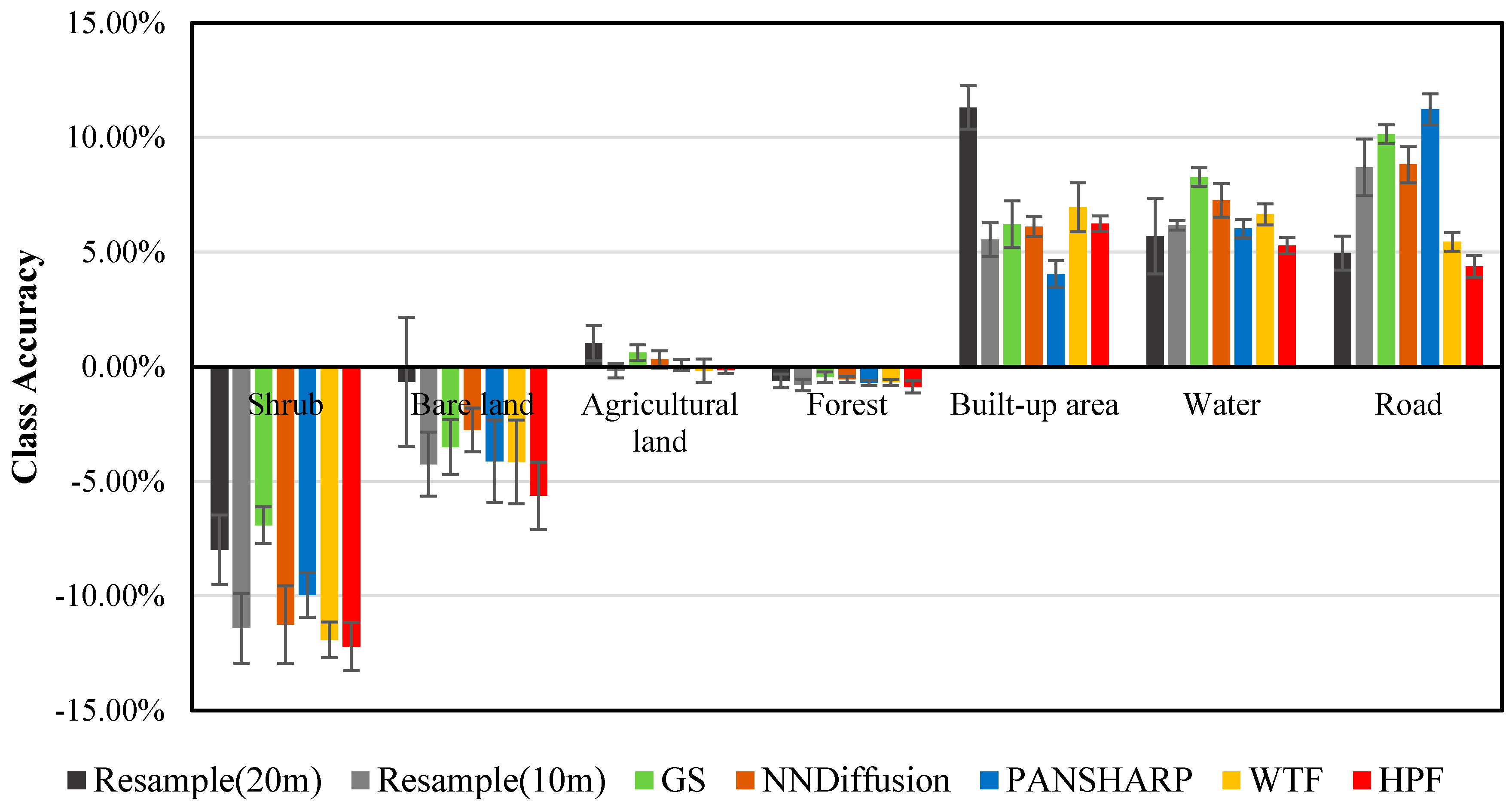
4.2. Effects of Downscaling Algorithms

For Sentinel-2, first, the effect of image sharpening on classification accuracy improvement is negligible. As shown in Table 5, based solely on spectral bands, HPF achieved the best accuracy than other pansharpening algorithms with an OA of 90.54% and Kappa of 0.88. Nevertheless, it is almost the same with the benchmark image downscaled by nearest neighbor resampling, which achieved an overall accuracy of 90.33% and Kappa of 0.87. This result is inconsistent with that obtained from MODIS and ASTER [27], because the classification accuracy is not only affected by the different spectral fidelity of these pansharpening algorithms, but also influenced by the classification system and the characteristics of the Sentinel-2 data, and they can be illustrated by the global feature importance, as shown in Figure 5 [68]. The most important features contain bands 2, 3, 4, 11, and 12, where only two of them were sharpened. As feature importance represents its contribution to distinguish the different classes, it demonstrates that for our classification system that only contains major land cover and land use types, the original four 10-m bands can already well discriminate these classes. Compared to MODIS and ASTER, the more fine resolution bands of Sentinel-2 makes it of great convenience and potential in regional LULC mapping.
Second, because of the sensor dependence in spectral fidelity and spatial enhancement of different pansharpening algorithms, their effects on classification accuracy for Sentinel-2 imagery is distinct from that for other data. For example, the accuracies of NNDiffusion and PANSHARP are almost the same as GS, which illustrates that, for Sentinel-2, the statistics-based pansharpening algorithms have the same effect on classification accuracy as the one based on CS. It is inconsistent with the conclusion which has been proved on WordView-2, GeoEye-1, Landsat 7(ETM+), IKONOS, and QuickBird [23,53]. That is because the spectral preservation capability of statistics-based algorithms is greatly limited by the spectral overlaps between the MS image and the PAN band. For Sentinel-2, only two of six bands at a 20-m GSD (bands 7 and 8a) have a spectral overlap with the PAN-like band (band8), resulting in a poor performance compared to the images with a PAN band. In addition, the MRA-based pansharpening algorithms can achieve a better spectral and spatial quality than those based on CS. This finding is consistent with other studies that used other sensor’s data [69].
In addition to the promotion to overall accuracy, image sharpening can also benefit some specific LULC classes. Figure 6 illustrates the accuracy of each class obtained by different downscaling methods. We can easily observe that image sharpening has advantages in class road with the classification accuracy increased by 3.8% with HPF and WTF and that the HPF also has a slight superiority in water. In contrast, image sharpening also has an obvious disadvantage in the shrub, bare land, and built-up areas.

4.3. Effects of Spatial Features

The spatial features were added to take full advantage of increased spatial details from image sharpening and to fully evaluate the potential of image sharpening for LULC classification of Sentinel-2. Besides that, the effects of two spatial features on classification accuracy were also assessed using Sentinel-2 imagery for the first time. In general, GLCM and EAPs have an obvious advantage over image sharpening in classification accuracy of Sentinel-2. Table 5 and Figure 3 and Figure 4 illustrate that all the accuracy statistics are greatly increased after EAPs and GLCM were integrated separately or together independent from data sets. For example, the lowest improvement of EAPs was achieved on the upscaled image at a 20-m GSD with the OA increased by 3.42%, and the highest improvement was obtained on downscaled data by PANSHARP with the OA increased by 4.83%. GLCM achieved the lowest increase on the image sharpened by HPF with the OA increased by 4.25%, and its highest improvement was obtained on the image generated by GS with the OA increased by 6.23%.
They differ not only in the OA but also in different classes. In Figure 7, the columns above x-axis represent that GLCM has a better performance than EAPs on its corresponding classes, and below x-axis are the opposite. The higher the column, the greater their differences in accuracy promotion. From this bar chart, EAPs and GLCM have a similar effect on agricultural land and forest, but in built-up area, water and road, GLCM performs better, and EAPs reverses its disadvantages in shrub and agricultural land.

5. Conclusions

This paper assesses the effects of different spatial resolution unification schemes as well as spatial features on LULC classification accuracy using Sentinel-2 multi-resolution and multi-spectral images. For this purpose, one upscaling and six downscaling algorithms were used to generate seven data sets for classification. The spatial features of EAPs and GLCM were added to ensure an unbiased assessment by compensating for the shortcomings of image sharpening and spatial information loss in pixel-based classification. Their improvements in classification accuracy were investigated for the first time for Sentinel-2 imagery.
For Sentinel-2, downscaling based on even the most straightforward nearest neighbor resampling has an overwhelming superiority over upscaling in LULC classification. Therefore, we recommend the use of downscaling to unify the spatial resolution in data preprocessing for LULC classification of Sentinel-2.
For downscaling techniques, image sharpening has little effect on overall accuracy than spatial interpolation, and some of them even significantly underperform the resampling and are difficult to be applied. However, image sharpening algorithms outperform resampling in some specific classes, e.g., the two MRA-based methods, i.e., WTF and HPF, have obvious advantages than resampling in water and road, but at the cost of a lower accuracy in shrub, bare land, and built-up area. For image sharpening, the NNDiffusion and PANSHARP based on statistics achieved a similar accuracy as the GS method based on CS, and both of them underperform WTF and HPF, which are based on MRA.
Both EAPs and GLCM can significantly improve the LULC classification accuracy of Sentinel-2 imagery. The best accuracy can be achieved by adding both of them, similar to the findings in the previous literature. Although their improvements on overall accuracy are similar, the effectiveness to specific classes differ greatly. GLCM has a better performance in built-up area, water, and road, whereas EAPs contribute to a higher improvement in shrub and bare land. In agricultural land and forest, which already achieved a high precision, their effects are similar.
Although the spatial features have a significant effect on the accuracy of some specific classes, considering the computational complexity and the limited benefit of image sharpening, the image downscaled by nearest neighbor interpolation solely based on spectral bands can already meet the requirement of regional LULC applications. The EAPs and GLCM can be integrated with spectral bands separately or together for the applications that have a specific requirement to some certain classes. The most accuracy LULC map achieved by the downscaled image by HPF with the spatial features of EAPs and GLCM as shown in Figure 8.
Our further study will focus on establishing a hierarchical classification system that aims at discriminating more vegetation species, where the 20-m bands of Sentinel-2 (e.g., the three unique red-edge bands) have more contributions, to evaluate the potential of image sharpening in classifying different crops, trees, and other vegetation species.

Acknowledgments

This work is supported by Natural Science Foundation of China (No. 41631176). Thanks to the anonymous reviewers and the editor for their constructive comments and helpful suggestions, which have greatly improved this manuscript.

Author Contributions

Hongrui Zheng, Peijun Du, Jike Chen and Junshi Xia conceived and designed the experiments; Hongrui Zheng and Jike Chen performed the experiments; Hongrui Zheng and Jike Chen analyzed the data; Xiaojuan Li contributed analysis tools; Zhigang Xu and Naoto Yokoya provided many helpful suggestions and modified this manuscript very seriously; Hongrui Zheng and Peijun Du wrote the paper.

Conflicts of Interest

The authors declare no conflict of interest.

References

  1. Cihlar, J. Land cover mapping of large areas from satellites: Status and research priorities. Int. J. Remote Sens. 2000, 21, 1093–1114. [Google Scholar] [CrossRef]
  2. Rogan, J.; Chen, D. Remote sensing technology for mapping and monitoring land-cover and land-use change. Prog. Plan. 2004, 61, 301–325. [Google Scholar] [CrossRef]
  3. Wang, Q.; Blackburn, G.A.; Onojeghuo, A.O.; Dash, J.; Zhou, L.; Zhang, Y.; Atkinson, P.M. Fusion of landsat 8 oli and sentinel-2 MSI data. IEEE Trans. Geosci. Remote Sens. 2017. [Google Scholar] [CrossRef]
  4. Vincini, M.; Amaducci, S.; Frazzi, E. Empirical estimation of leaf chlorophyll density in winter wheat canopies using sentinel-2 spectral resolution. IEEE Trans. Geosci. Remote Sens. 2014, 52, 3220–3235. [Google Scholar] [CrossRef]
  5. Fernandes, R.; Weiss, M.; Camacho, F.; Berthelot, B.; Baret, F.; Duca, R. Development and assessment of leaf area index algorithms for the sentinel-2 multispectral imager. In Proceedings of the 2014 IEEE International Geoscience and Remote Sensing Symposium (IGARSS), Quebec City, QC, Canada, 13–18 July 2014; pp. 3922–3925. [Google Scholar]
  6. Toming, K.; Kutser, T.; Laas, A.; Sepp, M.; Paavel, B.; Nõges, T. First experiences in mapping lake water quality parameters with sentinel-2 MSI imagery. Remote Sens. 2016, 8, 640. [Google Scholar] [CrossRef]
  7. Du, Y.; Zhang, Y.; Ling, F.; Wang, Q.; Li, W.; Li, X. Water bodies’ mapping from sentinel-2 imagery with modified normalized difference water index at 10-m spatial resolution produced by sharpening the swir band. Remote Sens. 2016, 8, 354. [Google Scholar] [CrossRef] [Green Version]
  8. Kaplan, G.; Avdan, U. Object-based water body extraction model using sentinel-2 satellite imagery. Eur. J. Remote Sens. 2017, 50, 137–143. [Google Scholar] [CrossRef]
  9. Novelli, A.; Aguilar, M.A.; Nemmaoui, A.; Aguilar, F.J.; Tarantino, E. Performance evaluation of object based greenhouse detection from sentinel-2 MSI and landsat 8 oli data: A case study from almería (Spain). Int. J. Appl. Earth Obs. Geoinf. 2016, 52, 403–411. [Google Scholar] [CrossRef]
  10. Pesaresi, M.; Corbane, C.; Julea, A.; Florczyk, A.J.; Syrris, V.; Soille, P. Assessment of the added-value of sentinel-2 for detecting built-up areas. Remote Sens. 2016, 8, 299. [Google Scholar] [CrossRef] [Green Version]
  11. Immitzer, M.; Vuolo, F.; Atzberger, C. First experience with sentinel-2 data for crop and tree species classifications in central europe. Remote Sens. 2016, 8, 166. [Google Scholar] [CrossRef]
  12. Sibanda, M.; Mutanga, O.; Rouget, M. Examining the potential of sentinel-2 MSI spectral resolution in quantifying above ground biomass across different fertilizer treatments. ISPRS J. Photogramm. Remote Sens. 2015, 110, 55–65. [Google Scholar] [CrossRef]
  13. Wang, Q.; Shi, W.; Atkinson, P.M.; Zhao, Y. Downscaling modis images with area-to-point regression kriging. Remote Sens. Environ. 2015, 166, 191–204. [Google Scholar] [CrossRef]
  14. Rowan, L.C.; Mars, J.C. Lithologic mapping in the mountain pass, california area using advanced spaceborne thermal emission and reflection radiometer (ASTER) data. Remote Sens. Environ. 2003, 84, 350–366. [Google Scholar] [CrossRef]
  15. Pour, A.B.; Hashim, M. Identification of hydrothermal alteration minerals for exploring of porphyry copper deposit using ASTER data, se iran. J. Asian Earth Sci. 2011, 42, 1309–1323. [Google Scholar] [CrossRef]
  16. Atkinson, P.M. Downscaling in remote sensing. Int. J. Appl. Earth Obs. Geoinf. 2013, 22, 106–114. [Google Scholar] [CrossRef]
  17. Parker, J.A.; Kenyon, R.V.; Troxel, D.E. Comparison of interpolating methods for image resampling. IEEE Trans. Med. Imaging 1983, 2, 31–39. [Google Scholar] [CrossRef] [PubMed]
  18. Roy, D.; Dikshit, O. Investigation of image resampling effects upon the textural information content of a high spatial resolution remotely sensed image. Int. J. Remote Sens. 1994, 15, 1123–1130. [Google Scholar] [CrossRef]
  19. Sirguey, P.; Mathieu, R.; Arnaud, Y.; Khan, M.M.; Chanussot, J. Improving modis spatial resolution for snow mapping using wavelet fusion and arsis concept. IEEE Geosci. Remote Sens. Lett. 2008, 5, 78–82. [Google Scholar] [CrossRef] [Green Version]
  20. Laben, C.A.; Brower, B.V. Process for Enhancing the Spatial Resolution of Multispectral Imagery Using Pan-Sharpening. U.S. Patent 6,011,875, 4 January 2000. [Google Scholar]
  21. Wald, L.; Ranchin, T.; Mangolini, M. Fusion of satellite images of different spatial resolutions: Assessing the quality of resulting images. Photogramm. Eng. Remote Sens. 1997, 63, 691–699. [Google Scholar]
  22. Amro, I.; Mateos, J.; Vega, M.; Molina, R.; Katsaggelos, A.K. A survey of classical methods and new trends in pansharpening of multispectral images. EURASIP J. Adv. Signal Process. 2011, 2011, 79. [Google Scholar] [CrossRef]
  23. Zhang, Y. Understanding image fusion. Photogramm. Eng. Remote Sens. 2004, 70, 657–661. [Google Scholar]
  24. Pohl, C.; van Genderen, J. Review article multisensor image fusion in remote sensing: Concepts, methods and applications. Int. J. Remote Sens. 1998, 19, 823–854. [Google Scholar] [CrossRef]
  25. Alparone, L.; Wald, L.; Chanussot, J.; Thomas, C.; Gamba, P.; Bruce, L.M. Comparison of pansharpening algorithms: Outcome of the 2006 grs-s data-fusion contest. IEEE Trans. Geosci. Remote Sens. 2007, 45, 3012–3021. [Google Scholar] [CrossRef] [Green Version]
  26. Welch, R.; Ehlers, M. Merging multiresolution spot hrv and landsat tm data. Photogramm. Eng. Remote Sens. 1987, 53, 301–303. [Google Scholar]
  27. Kim, S.-H.; Kang, S.-J.; Lee, K.-S. Comparison of fusion methods for generating 250 m modis image. Korean J. Remote Sens. 2010, 26, 305–316. [Google Scholar]
  28. Gilbertson, J.K.; Kemp, J.; Van Niekerk, A. Effect of pan-sharpening multi-temporal landsat 8 imagery for crop type differentiation using different classification techniques. Comput. Electron. Agric. 2017, 134, 151–159. [Google Scholar] [CrossRef]
  29. Wang, Q.; Shi, W.; Li, Z.; Atkinson, P.M. Fusion of sentinel-2 images. Remote Sens. Environ. 2016, 187, 241–252. [Google Scholar] [CrossRef]
  30. Pereira, M.J.; Ramos, A.; Nunes, R.; Azevedo, L.; Soares, A. Geostatistical data fusion: Application to red edge bands of sentinel 2. In Proceedings of the 2016 International Conference on Computational Science and Computational Intelligence (CSCI), Las Vegas, NV, USA, 15–17 December 2016; pp. 758–761. [Google Scholar]
  31. Vaiopoulos, A.D.; Karantzalos, K. Pansharpening on the narrow vnir and swir spectral bands of sentinel-2. ISPRS Int. Arch. Photogramm. Remote Sens. Spat. Inf. Sci. 2016, XLI-B7, 723–730. [Google Scholar] [CrossRef]
  32. Blaschke, T.; Lang, S.; Lorup, E.; Strobl, J.; Zeil, P. Object-oriented image processing in an integrated gis/remote sensing environment and perspectives for environmental applications. Environ. Inf. Plan. Politics Public 2000, 2, 555–570. [Google Scholar]
  33. Yan, G.; Mas, J.F.; Maathuis, B.H.P.; Xiangmin, Z.; Van Dijk, P.M. Comparison of pixel-based and object-oriented image classification approaches—A case study in a coal fire area, Wuda, Inner Mongolia, China. Int. J. Remote Sens. 2006, 27, 4039–4055. [Google Scholar] [CrossRef]
  34. Pedergnana, M.; Marpu, P.R.; Dalla Mura, M.; Benediktsson, J.A.; Bruzzone, L. Classification of remote sensing optical and lidar data using extended attribute profiles. IEEE J. Sel. Top. Signal Process. 2012, 6, 856–865. [Google Scholar] [CrossRef]
  35. Du, P.; Samat, A.; Waske, B.; Liu, S.; Li, Z. Random forest and rotation forest for fully polarized SAR image classification using polarimetric and spatial features. ISPRS J. Photogramm. Remote Sens. 2015, 105, 38–53. [Google Scholar] [CrossRef]
  36. Marceau, D.J.; Howarth, P.J.; Dubois, J.-M.M.; Gratton, D.J. Evaluation of the grey-level co-occurrence matrix method for land-cover classification using spot imagery. IEEE Trans. Geosci. Remote Sens. 1990, 28, 513–519. [Google Scholar] [CrossRef]
  37. Zhang, Y. Optimisation of building detection in satellite images by combining multispectral classification and texture filtering. ISPRS J. Photogramm. Remote Sens. 1999, 54, 50–60. [Google Scholar] [CrossRef]
  38. Gong, P.; Marceau, D.J.; Howarth, P.J. A comparison of spatial feature extraction algorithms for land-use classification with spot hrv data. Remote Sens. Environ. 1992, 40, 137–151. [Google Scholar] [CrossRef]
  39. Puissant, A.; Hirsch, J.; Weber, C. The utility of texture analysis to improve per-pixel classification for high to very high spatial resolution imagery. Int. J. Remote Sens. 2005, 26, 733–745. [Google Scholar] [CrossRef]
  40. Benediktsson, J.A.; Pesaresi, M.; Amason, K. Classification and feature extraction for remote sensing images from urban areas based on morphological transformations. IEEE Trans. Geosci. Remote Sens. 2003, 41, 1940–1949. [Google Scholar] [CrossRef]
  41. Benediktsson, J.A.; Palmason, J.A.; Sveinsson, J.R. Classification of hyperspectral data from urban areas based on extended morphological profiles. IEEE Trans. Geosci. Remote Sens. 2005, 43, 480–491. [Google Scholar] [CrossRef]
  42. Dalla Mura, M.; Atli Benediktsson, J.; Waske, B.; Bruzzone, L. Extended profiles with morphological attribute filters for the analysis of hyperspectral data. Int. J. Remote Sens. 2010, 31, 5975–5991. [Google Scholar] [CrossRef]
  43. Dalla Mura, M.; Benediktsson, J.A.; Waske, B.; Bruzzone, L. Morphological attribute profiles for the analysis of very high resolution images. IEEE Trans. Geosci. Remote Sens. 2010, 48, 3747–3762. [Google Scholar] [CrossRef]
  44. Dalla Mura, M.; Villa, A.; Benediktsson, J.A.; Chanussot, J.; Bruzzone, L. Classification of hyperspectral images by using extended morphological attribute profiles and independent component analysis. IEEE Geosci. Remote Sens. Lett. 2011, 8, 542–546. [Google Scholar] [CrossRef]
  45. Ghamisi, P.; Benediktsson, J.A.; Cavallaro, G.; Plaza, A. Automatic framework for spectral-spatial classification based on supervised feature extraction and morphological attribute profiles. IEEE J. Sel. Top. Appl. Earth Obs. Remote Sens. 2014, 7, 2147–2160. [Google Scholar] [CrossRef]
  46. Ghamisi, P.; Benediktsson, J.A.; Sveinsson, J.R. Automatic spectral-spatial classification framework based on attribute profiles and supervised feature extraction. IEEE Trans. Geosci. Remote Sens. 2014, 52, 5771–5782. [Google Scholar] [CrossRef]
  47. Qin, B.; Zhu, G.; Gao, G.; Zhang, Y.; Li, W.; Paerl, H.W.; Carmichael, W.W. A drinking water crisis in lake taihu, china: Linkage to climatic variability and lake management. Environ. Manag. 2010, 45, 105–112. [Google Scholar] [CrossRef] [PubMed]
  48. Zhang, Y.; Yin, Y.; Liu, X.; Shi, Z.; Feng, L.; Liu, M.; Zhu, G.; Gong, Z.; Qin, B. Spatial-seasonal dynamics of chromophoric dissolved organic matter in lake taihu, a large eutrophic, shallow lake in china. Org. Geochem. 2011, 42, 510–519. [Google Scholar] [CrossRef]
  49. Wan, R.; Cai, S.; Li, H.; Yang, G.; Li, Z.; Nie, X. Inferring land use and land cover impact on stream water quality using a bayesian hierarchical modeling approach in the Xitiaoxi River Watershed, China. J. Environ. Manag. 2014, 133, 1–11. [Google Scholar] [CrossRef] [PubMed]
  50. Drusch, M.; Del Bello, U.; Carlier, S.; Colin, O.; Fernandez, V.; Gascon, F.; Hoersch, B.; Isola, C.; Laberinti, P.; Martimort, P. Sentinel-2: Esa’s optical high-resolution mission for gmes operational services. Remote Sens. Environ. 2012, 120, 25–36. [Google Scholar] [CrossRef]
  51. Muller-Wilm, U.; Louis, J.; Richter, R.; Gascon, F.; Niezette, M. Sentinel-2 level 2a prototype processor: Architecture, algorithms and first results. In Proceedings of the 2013 ESA Living Planet Symposium, Edinburgh, UK, 9–13 September 2013; pp. 9–13. [Google Scholar]
  52. Zhang, Y.; Mishra, R.K. A review and comparison of commercially available pan-sharpening techniques for high resolution satellite image fusion. In Proceedings of the 2012 IEEE International Geoscience and Remote Sensing Symposium (IGARSS), Munich, Germany, 22–27 July 2012; pp. 182–185. [Google Scholar]
  53. Sun, W.; Chen, B.; Messinger, D.W. Nearest-neighbor diffusion-based pan-sharpening algorithm for spectral images. Opt. Eng. 2014, 53, 013107. [Google Scholar] [CrossRef]
  54. Lemeshewsky, G.P. Multispectral multisensor image fusion using wavelet transforms. Proc. SPIE Int. Soc. Opt. Eng. 1999, 3716, 214–222. [Google Scholar] [CrossRef]
  55. Gangkofner, U.G.; Pradhan, P.S.; Holcomb, D.W. Optimizing the high-pass filter addition technique for image fusion. Photogramm. Eng. Remote Sens. 2008, 74, 1107–1118. [Google Scholar] [CrossRef]
  56. Nunez, J.; Otazu, X.; Fors, O.; Prades, A.; Pala, V.; Arbiol, R. Multiresolution-based image fusion with additive wavelet decomposition. IEEE Trans. Geosci. Remote Sens. 1999, 37, 1204–1211. [Google Scholar] [CrossRef] [Green Version]
  57. Aiazzi, B.; Alparone, L.; Baronti, S.; Garzelli, A. Context-driven fusion of high spatial and spectral resolution images based on oversampled multiresolution analysis. IEEE Trans. Geosci. Remote Sens. 2002, 40, 2300–2312. [Google Scholar] [CrossRef]
  58. Haralick, R.M.; Shanmugam, K.; Dinstein, I. Textural features for image classification. Syst. Man Cybern. 1973, 3, 610–621. [Google Scholar] [CrossRef]
  59. Breiman, L. Random forest. Mach. Learn. 2001, 45, 5–32. [Google Scholar] [CrossRef]
  60. Pal, M. Random forest classifier for remote sensing classification. Int. J. Remote Sens. 2005, 26, 217–222. [Google Scholar] [CrossRef]
  61. Gomariz-Castillo, F.; Alonso-Sarría, F.; Cánovas-García, F. Improving classification accuracy of multi-temporal landsat images by assessing the use of different algorithms, textural and ancillary information for a mediterranean semiarid area from 2000 to 2015. Remote Sens. 2017, 9, 1058. [Google Scholar] [CrossRef]
  62. Genuer, R.; Poggi, J.-M.; Tuleau-Malot, C. Variable selection using random forests. Pattern Recognit. Lett. 2010, 31, 2225–2236. [Google Scholar] [CrossRef]
  63. Dietterich, T.G. Ensemble methods in machine learning. Mult. Classif. Syst. 2000, 1857, 1–15. [Google Scholar] [CrossRef]
  64. Lu, D.; Weng, Q. A survey of image classification methods and techniques for improving classification performance. Int. J. Remote Sens. 2007, 28, 823–870. [Google Scholar] [CrossRef]
  65. Thomlinson, J.R.; Bolstad, P.V.; Cohen, W.B. Coordinating methodologies for scaling landcover classifications from site-specific to global: Steps toward validating global map products. Remote Sens. Environ. 1999, 70, 16–28. [Google Scholar] [CrossRef]
  66. Irons, J.R.; Markham, B.L.; Nelson, R.F.; Toll, D.L.; Williams, D.L.; Latty, R.S.; Stauffer, M.L. The effects of spatial resolution on the classification of thematic mapper data. Int. J. Remote Sens. 1985, 6, 1385–1403. [Google Scholar] [CrossRef]
  67. Teruiya, R.; Paradella, W.; Dos Santos, A.; Dall’Agnol, R.; Veneziani, P. Integrating airborne SAR, landsat TM and airborne geophysics data for improving geological mapping in the amazon region: The cigano granite, Carajás Province, Brazil. Int. J. Remote Sens. 2008, 29, 3957–3974. [Google Scholar] [CrossRef]
  68. Congalton, R.G. A review of assessing the accuracy of classification of remotely sensed data. Work. Pap. 1991, 119, 270–279. [Google Scholar] [CrossRef]
  69. Colditz, R.R.; Wehrmann, T.; Bachmann, M.; Steinnocher, K.; Schmidt, M.; Strunz, G.; Dech, S. Influence of image fusion approaches on classification accuracy: A case study. Int. J. Remote Sens. 2006, 27, 3311–3335. [Google Scholar] [CrossRef]
Figure 1. Location of the Xitiaoxi watershed and Taihu Basin. The Sentinel-2 Multispectral Instrument (MSI) imagery is shown with true-color composite of Red, Green, and Blue bands in Bottom-of-Atmosphere reflectance data.
Remotesensing 09 01274 g001
Figure 2. Technical flow chart.
Remotesensing 09 01274 g002
Figure 3. Overall accuracy of seven preprocessed images on each of the feature sets.
Remotesensing 09 01274 g003
Figure 4. Kappa coefficient of seven preprocessed images on each of the feature sets.
Remotesensing 09 01274 g004
Figure 5. Feature importance of ten spectral bands using data sets obtained by six downscaling methods.
Remotesensing 09 01274 g005
Figure 6. Class accuracy using data sets obtained by different downscaling methods.
Remotesensing 09 01274 g006
Figure 7. Differences between extended attribute profiles (EAPs) and Grey-Level-Co-occurrence Matrix (GLCM) on class accuracy. Columns above x-axis stand for adding GLCM achieved a higher accuracy than EAPs on their corresponding classes, and those below x-axis are the opposite.
Remotesensing 09 01274 g007
Figure 8. LULC mapping generated by adding EAPs and GLCM with spectral bands of Sentinel-2 imagery sharpened by high-pass filter (HPF) fusion.
Remotesensing 09 01274 g008
Table 1. Data sets generated by preprocessing.
Geometric Unification SchemesMethodsResolutionAbbreviation
Spatial interpolationNearest neighbor resample20 mR20
Nearest neighbor resample10 mR10
Pan-sharpeningGSG10
NNDiffusionN10
PANSHARPP10
HPF fusionH10
Wavelet fusionW10
Table 2. The optimal PAN-like bands for each 20-m band determined by center wavelength proximity and bands correlation of Sentinel-2 (two image tiles were distinguished by colors).
Low-Resolution BandLike-PAN Band Based on Center Wavelength ProximityLike-PAN Band Based on Band Correlation
Band5Band4Band4Band4Band8
Band6Band8
Band7Band8Band8
Band8a
Band11
Band12Band4
Table 3. The combination schemes of each data and feature sets of all twenty eight classification scenarios.
Input VariableR20R10G10N10P10H10W10
F1F2F3F4F1F2F3F4F1F2F3F4F1F2F3F4F1F2F3F4F1F2F3F4F1F2F3F4
Spectral
EAPs
GLCM
Table 4. Number of training and validation pixels.
Training PixelsValidation PixelsPercentage
ClassesNumberNumber%
Shrub28825876.2
Bare land18316463.94
Agricultural land118210,63625.47
Forest152013,67532.75
Built-up area42538259.16
Water34430947.41
Road699629315.06
Total464141,756100
Table 5. Classification accuracies (in percentage, OA: overall accuracy, Kappa: kappa coefficient).
OAKappaShrubBare LandAgriculture LandForestBuilt up AreaWaterRoad
F1R2086.690.8373.2658.4392.3096.7170.6590.7676.13
R1090.330.8779.4972.5094.5397.8279.1491.6779.85
G1088.540.8578.3168.0093.5497.4573.1787.8176.06
N1088.590.8577.5068.3793.2697.5773.4390.3375.32
P1088.530.8578.2667.9093.5297.5072.3590.7374.83
W1090.160.8777.9767.8594.4397.7473.7391.5383.52
H1090.540.8877.1168.7594.7797.7276.1892.7783.65
F2R2089.920.8784.1571.6294.0497.4374.8490.2882.92
R1093.820.9292.1583.6996.9298.6384.1392.0285.97
G1092.840.9188.8483.9996.5498.3282.8590.2483.39
N1093.320.9191.3382.4196.6998.5083.1791.1384.86
P1093.360.9190.7785.0196.7498.6183.2692.3583.49
W1094.180.9292.0483.9097.2498.6982.6091.8388.90
H1094.610.9392.6883.5297.2998.8284.1593.5289.62
F3R2091.670.8976.1670.9695.0796.8186.1595.9887.75
R1094.720.9380.7579.4496.7597.8489.6898.1894.67
G1094.770.9381.9380.4897.1597.8889.0798.5293.53
N1094.640.9380.0879.6697.0097.9689.2798.3893.68
P1094.650.9380.8280.8996.8297.9187.3198.3894.71
W1094.800.9380.1279.7497.0798.0189.5598.4794.35
H1094.790.9380.4777.8897.1497.9490.3998.7994.00
F4R2092.990.9182.2973.5496.3297.0186.9595.3890.60
R1096.030.9589.1682.7897.8398.3291.9197.7995.14
G1095.950.9586.8185.5597.9798.2591.1798.2694.91
N1095.980.9588.3383.0697.8798.3391.5097.9995.15
P1096.040.9587.0785.9397.8998.3991.3598.0295.19
W1096.330.9589.3283.6898.1798.4892.9498.1195.55
H1096.390.9588.4683.3398.3398.4993.2298.2995.55

