Local Deep Hashing Matching of Aerial Images Based on Relative Distance and Absolute Distance Constraints

Abstract
:
1. Introduction
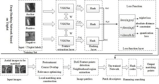
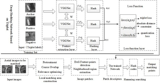
2. Proposed Method
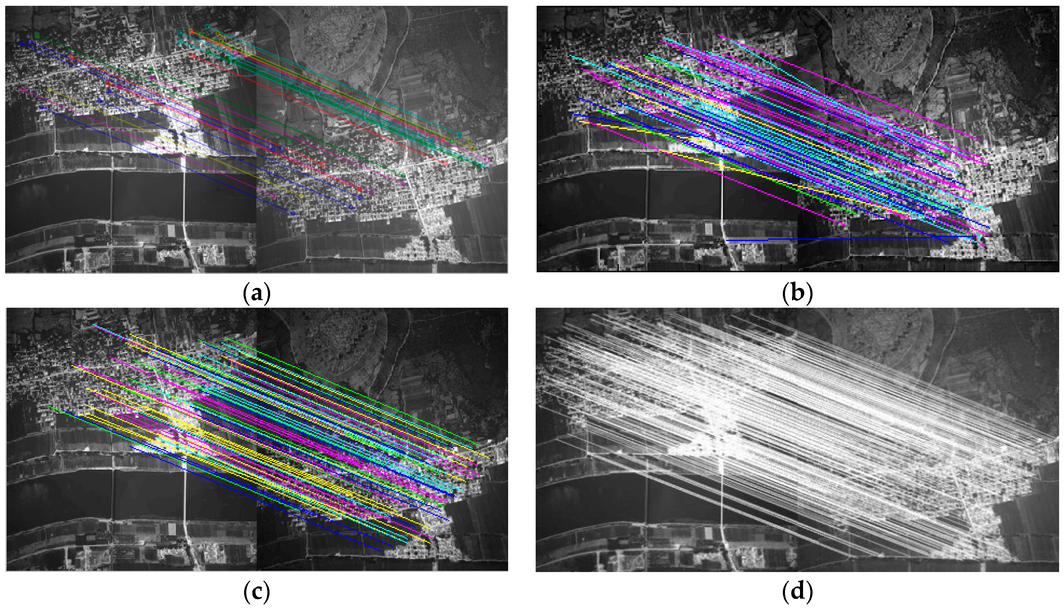
3. Construction of the Local Matching Region
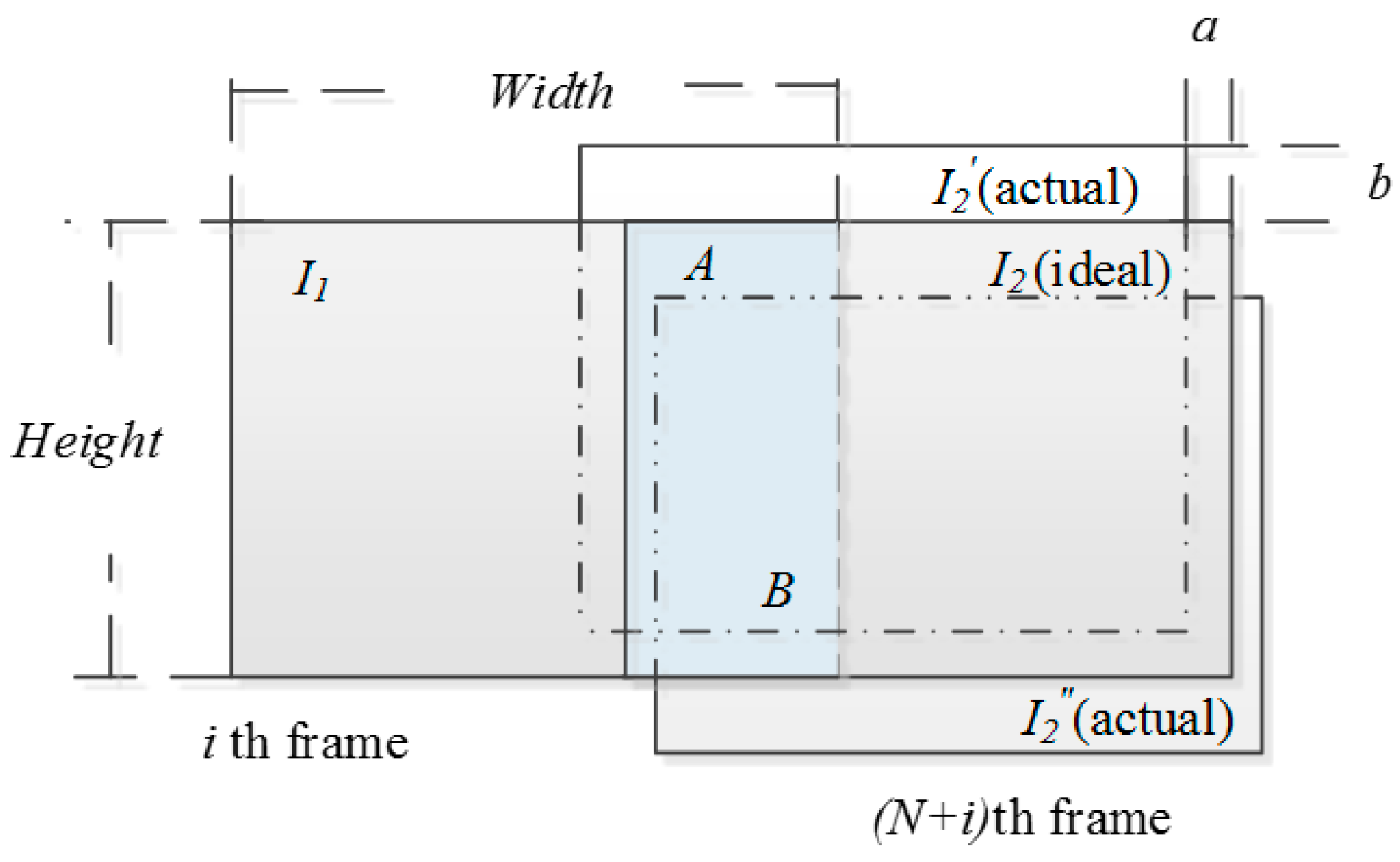
3.1. Construction of Initial Local Region
3.2. Local Region Optimization
| Algorithm 1: Construction of the local matching region of aerial images. |
| Input: , , image sequence , lateral shift step length , longitudinal shift step length , number of iterations and , |
| Output: The corresponding to maximum value is the actual overlapping region to be solved |
| Step1 Calculate the number of intervals N according to Equation (1) Step2 Denote the two aerial images to be matched , as and respectively, calculate the overlapping rate of the two images is Step3 According the new overlap rate, calculate the ideal overlapping region of and , denoted as and , the pixel size is Step4 Optimize local region For From To For From To According to Equation(2), calculate , = max(, ) End End |
4. Deep Hash Network Structure with Distance Constraint and Quantization Loss
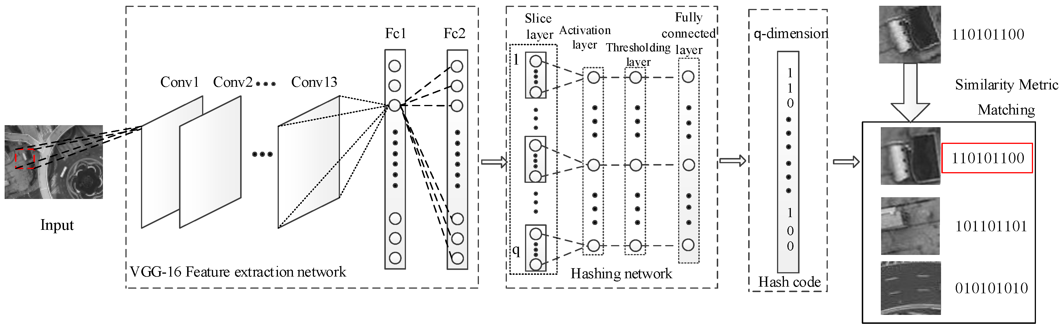
4.1. Independent Hashing Layer
4.2. New Objective Function
4.2.1. Classification Loss Based on the Absolute Distance Constraint
4.2.2. Quantization Loss
| Algorithm 2: LDHM algorithm |
| Input: Image training set , hash code dimension , number of iterations , weight , Output: The network matrix and the hash layer parameter, , |
| Step1 (Initialization) Use the VGG-Net model pre-trained in ImageNet to initialize the network, initialize the Hash Layer by randomly sampling from a Gaussian distribution with mean and variance ; |
| Step2 According to the network structure, calculate the deep feature representation ; Step3 Calculate ; Step4 Calculate the binary Hash code ; Step5 Calculate the derivative of the objective function (8), update the parameter , and the network matrix by back propagation; Step6 Repeat Step2~Step5 until the parameter value is invariable |
- Step 1: Local matching regions and are obtained from two aerial images to be matched and by Algorithm 1, as described in Section 3.
- Step 2: The DoG algorithm is used to detect the feature point in the local matching regions and , then the neighborhood patch of feature points is constructed with a size of 64 × 64 pixels.
- Step 3: According to Section 4, each image patch will be inputted to the trained network and represented by a binary hash code with better characterization and discrimination.
- Step 4: All feature patches in two local matching regions are represented by binary hash codes: for any feature in , its corresponding matching point in will be found by the approximate nearest neighbor search algorithm in the Hamming space, realizing the matching of aerial images.
5. Discussions
5.1. Experimental Sample Dataset
5.2. Evaluation Criterion
5.2.1. Precision Rate
5.2.2. Performance of the 95% Error Rate
5.2.3. Performance of the Matching Score
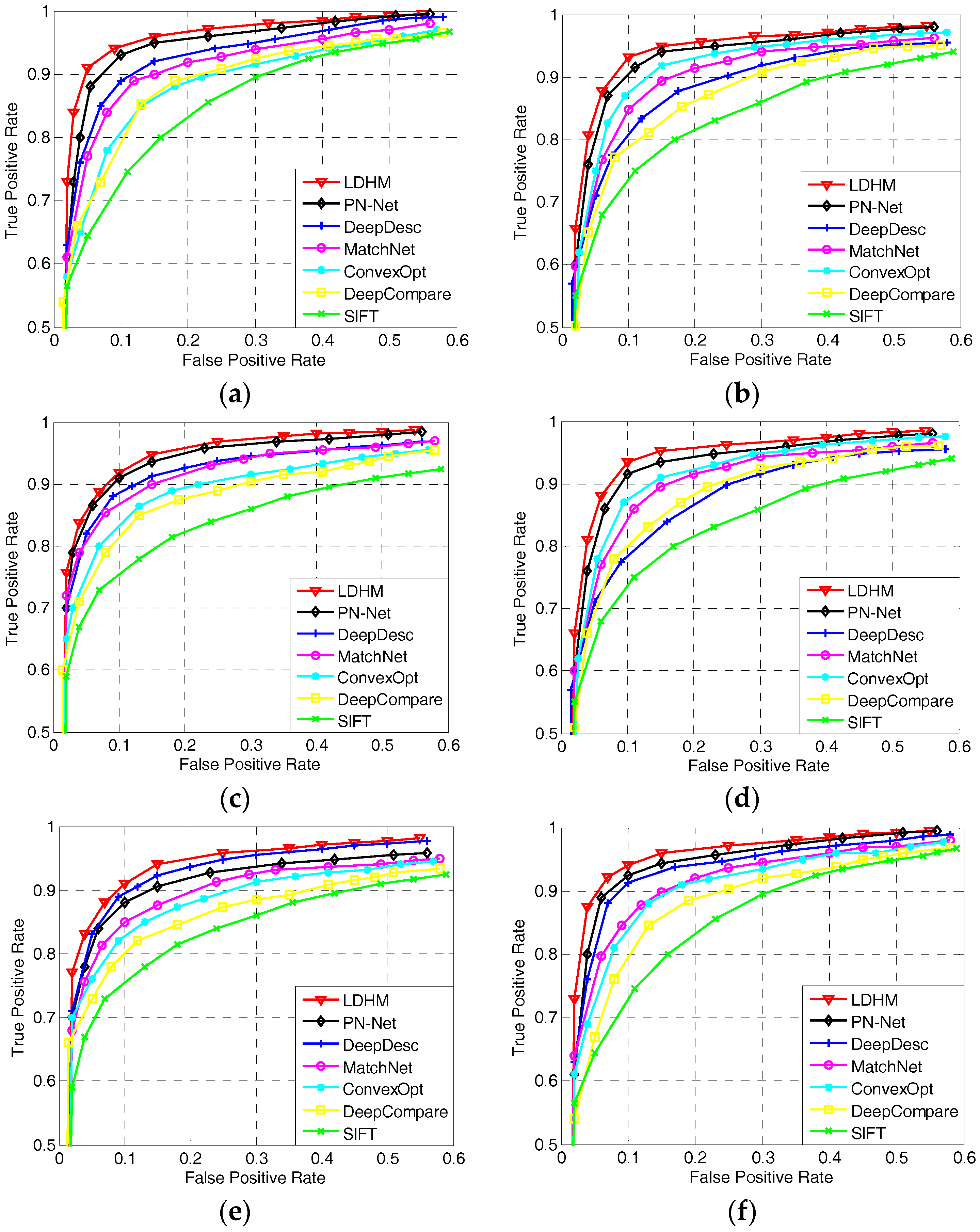
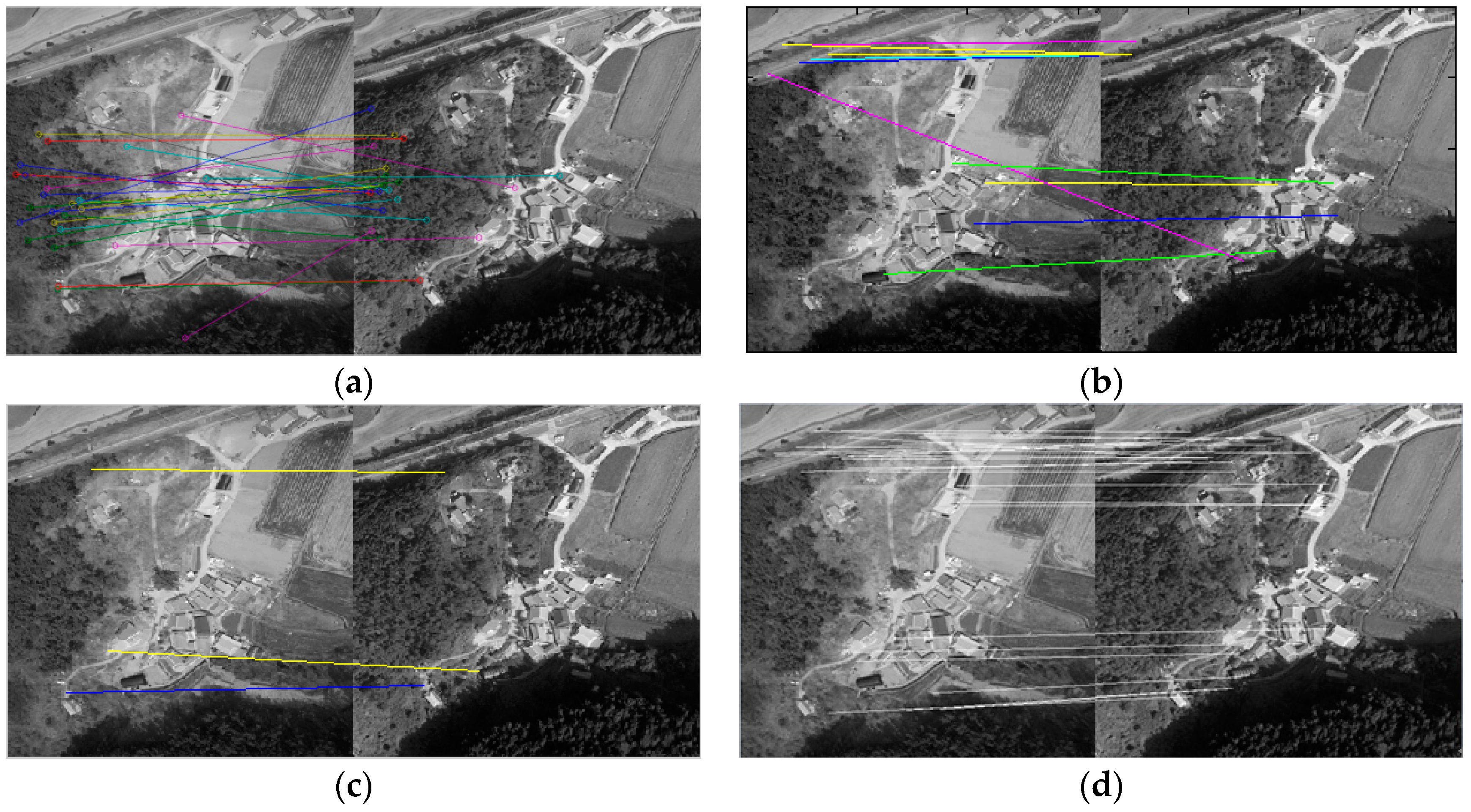
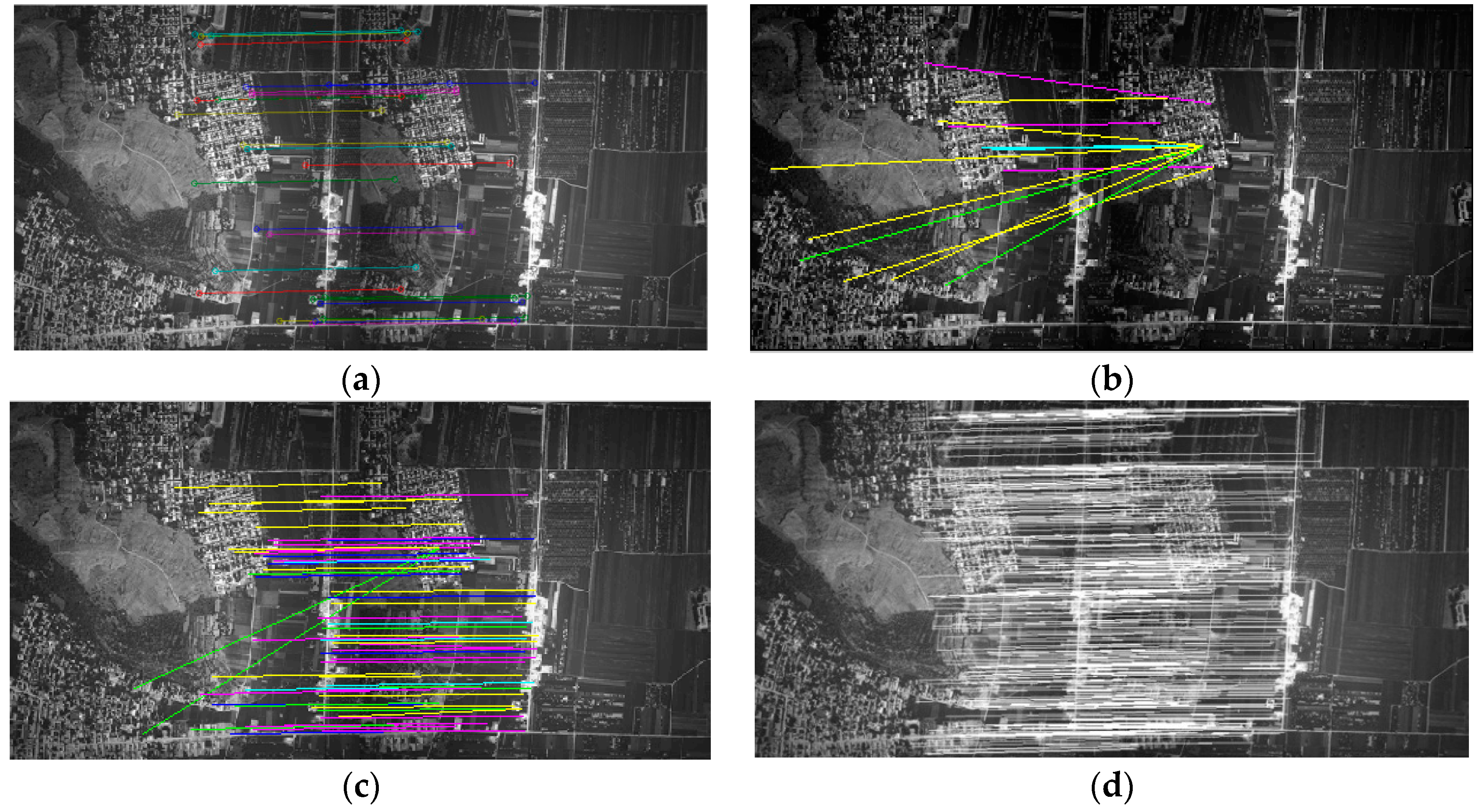
5.2.4. Comparison of the Matching Results
5.2.5. Comparison of Algorithm Efficiency
6. Conclusions
Acknowledgments
Author Contributions
Conflicts of Interest
References
- Yang, X.; Wang, J.; Qin, X.; Wang, J.; Ye, X.; Qin, Q. Fast urban aerial image matching based on rectangular building extraction. IEEE Geosci. Remote Sens. Mag. 2015, 3, 21–27. [Google Scholar] [CrossRef]
- Ren, X.; Sun, M.; Zhang, X.; Liu, L. A Simplified Method for UAV Multispectral Images Mosaicking. Remote Sens. 2017, 9, 962. [Google Scholar] [CrossRef]
- Lowe, D.G. Distinctive image features from scale-invariant keypoints. Int. J. Comput. Vis. 2004, 60, 91–110. [Google Scholar] [CrossRef]
- Calonder, M.; Lepetit, V.; Strecha, C.; Fua, P. Brief: Binary robust independent elementary features. Comput. Vis. ECCV 2010, 2010, 778–792. [Google Scholar]
- Rublee, E.; Rabaud, V.; Konolige, K.; Bradski, G. ORB: An efficient alternative to SIFT or SURF. In Proceedings of the 2011 IEEE International Conference on Computer Vision (ICCV), Barcelona, Spain, 6–13 November 2011; pp. 2564–2571. [Google Scholar]
- Bay, H.; Tuytelaars, T.; Gool, L.V. SURF: Speeded up robust features. Comput. Vis. ECCV 2006, 2006, 404–417. [Google Scholar]
- Sun, Y.; Zhao, L.; Huang, S.; Yan, L.; Dissanayake, G. L2-SIFT: SIFT feature extraction and matching for large images in large-scale aerial photogrammetry. ISPRS J. Photogramm. Remote Sens. 2014, 91, 1–16. [Google Scholar] [CrossRef]
- Liu, Z.; Wang, Y.; Jing, Y.; Lou, O. A robust feature point matching method for dynamic aerial Image registration. In Proceedings of the 2014 Sixth International Symposium on Parallel Architectures, Algorithms and Programming (PAAP), Beijing, China, 13–15 July 2014; pp. 144–147. [Google Scholar]
- Tsai, C.H.; Lin, Y.C. An accelerated image matching technique for UAV orthoimage registration. ISPRS J. Photogramm. Remote Sens. 2017, 128, 130–145. [Google Scholar] [CrossRef]
- Sedaghat, A.; Ebadi, H. Very high resolution image matching based on local features and k-means clustering. Photogramm. Rec. 2015, 30, 166–186. [Google Scholar] [CrossRef]
- Yang, K.; Pan, A.; Yang, Y.; Zhang, S.; Ong, S.H.; Tang, H. Remote Sensing Image Registration Using Multiple Image Features. Remote Sens. 2017, 9, 581. [Google Scholar] [CrossRef]
- Krizhevsky, A.; Sutskever, I.; Hinton, G.E. ImageNet classification with deep convolutional neural networks. In Advances in Neural Information Processing Systems; Curran Associates Inc.: New York, NY, USA, 2012; pp. 1097–1105. [Google Scholar]
- Zhou, W.; Newsam, S.; Li, C.; Shao, Z. Learning low dimensional convolutional neural networks for high-resolution remote sensing image retrieval. Remote Sens. 2016, 9, 489. [Google Scholar] [CrossRef]
- Kang, M.; Ji, K.; Leng, X.; Lin, Z. Contextual region-based convolutional neural network with multilayer fusion for SAR ship detection. Remote Sens. 2017, 9, 860. [Google Scholar] [CrossRef]
- Wang, Q.; Gao, J.; Yuan, Y. A joint convolutional neural networks and context transfer for street scenes labeling. IEEE Trans. Intell. Transp. Syst. 2017, 99, 1–14. [Google Scholar] [CrossRef]
- Wang, Q.; Gao, J.; Yuan, Y. Embedding structured contour and location prior in siamesed fully convolutional networks for road detection. In Proceedings of the IEEE International Conference on Robotics and Automation, Singapore, 29 May–3 June 2017; pp. 219–224. [Google Scholar]
- Babenko, A.; Slesarev, A.; Chigorin, A.; Lempitsky, V. Neural codes for image retrieval. In European Conference on Computer Vision, Proceedings of the 13th European Conference, Zurich, Switzerland, 6–12 September 2014; Springer: Cham, Switzerland, 2014; Volume 8689, pp. 584–599. [Google Scholar]
- Han, X.; Leung, T.; Jia, Y.; Sukthankar, R.; Berg, A.C. MatchNet: Unifying feature and metric learning for patch-based matching. In Proceedings of the IEEE Conference on Computer Vision and Pattern Recognition, Boston, MA, USA, 7–12 June 2015; pp. 3279–3286. [Google Scholar]
- Balntas, V.; Johns, E.; Tang, L.; Mikolajczyk, K. PN-Net: Conjoined triple deep network for learning local image descriptors. arXiv, 2016; arXiv:1601.05030. [Google Scholar]
- Ke, Y.; Sukthankar, R. PCA-SIFT: A More Distinctive Representation for Local Image Descriptors; IEEE: Piscataway, NJ, USA, 2004; pp. 506–513. [Google Scholar]
- Roweis, S.T.; Saul, L.K. Nonlinear dimensionality reduction by locally linear embedding. Science 2000, 290, 2323–2326. [Google Scholar] [CrossRef] [PubMed]
- Wang, Q.; Meng, Z.; Li, X. Locality adaptive discriminant analysis for spectral-spatial classification of hyperspectral images. IEEE Geosci. Remote Sens. Lett. 2017, 14, 2077–2081. [Google Scholar] [CrossRef]
- Peng, X.; Tang, H.; Zhang, L.; Yi, Z.; Xiao, S. A unified framework for representation-based subspace clustering of out-of-sample and large-scale data. IEEE Trans. Neural Netw. Learn. Syst. 2016, 27, 2499–2512. [Google Scholar] [CrossRef] [PubMed]
- Peng, X.; Yu, Z.; Yi, Z.; Tang, H. Constructing the L2-graph for robust subspace learning and subspace clustering. IEEE Trans. Cybern. 2017, 47, 1053–1066. [Google Scholar] [CrossRef] [PubMed]
- Peng, X.; Lu, J.; Yi, Z.; Yan, R. Automatic subspace learning via principal coefficients embedding. IEEE Trans. Cybern. 2014, 47, 3583–3596. [Google Scholar] [CrossRef] [PubMed]
- Li, W.; Zhou, Z. Learning to hash for big data: Current status and future trends. Chin. Sci. Bull. 2015, 60, 485–490. [Google Scholar] [CrossRef]
- Kong, W.; Li, W.J. Isotropic hashing. In Advances in Neural Information Processing Systems; NIPS: Barcelona, Spain, 2012; Volume 2, pp. 1646–1654. [Google Scholar]
- Weiss, Y.; Torralba, A.; Fergus, R. Spectral hashing. In Conference on Neural Information Processing Systems; NIPS: Barcelona, Spain, 2008; pp. 1753–1760. [Google Scholar]
- Lazebnik, S. Iterative quantization: A procrustean approach to learning binary codes. IEEE Trans. Pattern Anal. 2013, 12, 2916–2929. [Google Scholar]
- Wang, J.; Kumar, S.; Chang, S.F. Semi-supervised hashing for scalable image retrieval. In Proceedings of the IEEE Conference on Computer Vision and Pattern Recognition, San Francisco, CA, USA, 13–18 June 2010; pp. 3424–3431. [Google Scholar]
- Shen, F.; Shen, C.; Liu, W.; Shen, H.T. Supervised discrete hashing. In Proceedings of the IEEE Conference on Computer Vision and Pattern Recognition, Boston, MA, USA, 7–12 June 2015; pp. 37–45. [Google Scholar]
- Liu, W.; Wang, J.; Ji, R.; Jiang, Y.G.; Chang, S.F. Supervised hashing with kernels. In Proceedings of the IEEE Conference on Computer Vision and Pattern Recognition, Providence, RI, USA, 16–21 June 2012; pp. 2074–2081. [Google Scholar]
- Xia, R.; Pan, Y.; Lai, H.; Liu, C.; Yan, S. Supervised hashing for image retrieval via image representation learning. In Proceedings of the Twenty-Eighth AAAI Conference on Artificial Intelligence, Québec City, QC, Canada, 27–31 July 2014; pp. 2156–2162. [Google Scholar]
- Lai, H.; Pan, Y.; Liu, Y.; Yan, S. Simultaneous feature learning and hash coding with deep neural networks. In Proceedings of the IEEE Conference on Computer Vision and Pattern Recognition, Boston, MA, USA, 7–12 June 2015; pp. 3270–3278. [Google Scholar]
- Simonyan, K.; Zisserman, A. Very deep convolutional networks for large-scale image recognition. arXiv, 2014; arXiv:1409.1556. [Google Scholar]
- Liu, Z.; Li, Z.; Zhang, J.; Liu, L. Euclidean and hamming embedding for image patch description with convolutional networks. In Proceedings of the IEEE Conference on Computer Vision and Pattern Recognition Workshops, Las Vegas, NV, USA, 26 June–1 July 2016; pp. 1145–1151. [Google Scholar]
- Hoffer, E.; Ailon, N. Deep metric learning using triplet network. In Proceedings of the International Workshop on Similarity-Based Pattern Recognition, Copenhagen, Denmark, 12–14 October 2015; pp. 84–92. [Google Scholar]
- Balntas, V.; Riba, E.; Ponsa, D.; Mikolajczyk, K. Learning local feature descriptors with triplets and shallow convolutional neural networks. In Proceedings of the British Machine Vision Association (BMVC) 2016, York, UK, 19–22 September 2016; p. 3. [Google Scholar]
- Cakir, F.; Sclaroff, S. Adaptive hashing for fast similarity search. In Proceedings of the IEEE International Conference on Computer Vision, Santiago, Chile, 7–13 December 2015; pp. 1044–1052. [Google Scholar]
- Zagoruyko, S.; Komodakis, N. Learning to compare image patches via convolutional neural networks. In Proceedings of the IEEE Conference on Computer Vision and Pattern Recognition, Boston, MA, USA, 7–12 June 2015; pp. 4353–4361. [Google Scholar]
- Simoserra, E.; Trulls, E.; Ferraz, L.; Simo-Serra, E.; Trulls, E.; Ferraz, L.; Kokkinos, I.; Fua, P.; Moreno-Noguer, F. Discriminative learning of deep convolutional feature point descriptors. In Proceedings of the IEEE International Conference on Computer Vision, Santiago, Chile, 7–13 December 2015; pp. 118–126. [Google Scholar]
- Simonyan, K.; Vedaldi, A.; Zisserman, A. Learning local feature descriptors using convex optimisation. IEEE Trans. Pattern Anal. 2014, 36, 1573–1585. [Google Scholar] [CrossRef] [PubMed]


| Name | Image Pairs | Resolution (Pixel) | GSD (m) | Number (Ten Thousand) | Patch Size (Pixel) |
|---|---|---|---|---|---|
| Group 1 | UltraCam-D | 1256 × 1278 | 0.10 | 15 | 64 × 64 |
| UltraCam-D | 1256 × 1278 | 0.10 | 64 × 64 | ||
| Group 2 | UltraCam-D | 1161 × 1169 | 0.10 | 12 | 64 × 64 |
| UltraCam-D | 1161 × 1169 | 0.10 | 64 × 64 | ||
| Group 3 | UltraCam-D | 1197 × 1203 | 0.10 | 13 | 64 × 64 |
| UltraCam-D | 1197 × 1203 | 0.10 | 64 × 64 |
| Training Set | Group 2 | Group 3 | Group 1 | Group 3 | Group 1 | Group 2 | Average |
|---|---|---|---|---|---|---|---|
| Testing Set | Group 1 | Group 2 | Group 3 | 95% ERR | |||
| SIFT | 26.76 | 20.76 | 23.74 | 23.75 | |||
| Deep Desc | 7.93 | 5.64 | 14.05 | 9.21 | |||
| MatchNate | 7.93 | 12.32 | 5.35 | 8.65 | 12.63 | 10.06 | 9.49 |
| DeepCompare | 12.24 | 16.35 | 7.51 | 9.47 | 18.84 | 14.79 | 13.2 |
| PN-Net | 7.58 | 8.76 | 4.78 | 5.33 | 8.39 | 6.63 | 6.91 |
| CovexOpt | 10.72 | 13.68 | 7.24 | 8.27 | 10.37 | 9.24 | 9.92 |
| Proposed | 7.14 | 7.56 | 4.68 | 5.40 | 7.96 | 6.24 | 6.50 |
| Algorithm | SIFT | BRIEF | PN-Net | DeepCompare | MatchNet | Proposed |
|---|---|---|---|---|---|---|
| Group 1 | 0.301 | 0.194 | 0.322 | 0.313 | 0.247 | 0.329 |
| Group 2 | 0.294 | 0.184 | 0.310 | 0.304 | 0.238 | 0.322 |
| Group 3 | 0.281 | 0.171 | 0.289 | 0.293 | 0.225 | 0.305 |
| Average | 0.292 | 0.183 | 0.307 | 0.303 | 0.237 | 0.319 |
| Algorithm | SIFT | BRIEF | PN-Net | DeepCompare | MatchNet | Proposed |
|---|---|---|---|---|---|---|
| Time (ms) | 0.51 | 0.013 | 0.021 | 0.049 | 0.624 | 0.018 |
© 2017 by the authors. Licensee MDPI, Basel, Switzerland. This article is an open access article distributed under the terms and conditions of the Creative Commons Attribution (CC BY) license (http://creativecommons.org/licenses/by/4.0/).
Share and Cite
Chen, S.; Li, X.; Zhang, Y.; Feng, R.; Zhang, C. Local Deep Hashing Matching of Aerial Images Based on Relative Distance and Absolute Distance Constraints. Remote Sens. 2017, 9, 1244. https://doi.org/10.3390/rs9121244
Chen S, Li X, Zhang Y, Feng R, Zhang C. Local Deep Hashing Matching of Aerial Images Based on Relative Distance and Absolute Distance Constraints. Remote Sensing. 2017; 9(12):1244. https://doi.org/10.3390/rs9121244
Chicago/Turabian StyleChen, Suting, Xin Li, Yanyan Zhang, Rui Feng, and Chuang Zhang. 2017. "Local Deep Hashing Matching of Aerial Images Based on Relative Distance and Absolute Distance Constraints" Remote Sensing 9, no. 12: 1244. https://doi.org/10.3390/rs9121244
APA StyleChen, S., Li, X., Zhang, Y., Feng, R., & Zhang, C. (2017). Local Deep Hashing Matching of Aerial Images Based on Relative Distance and Absolute Distance Constraints. Remote Sensing, 9(12), 1244. https://doi.org/10.3390/rs9121244