Hyperspectral Image Segmentation via Frequency-Based Similarity for Mixed Noise Estimation

School of Computer Science and Engineering, Nanjing University of Science and Technology, Nanjing 210094, China
*
Authors to whom correspondence should be addressed.
Remote Sens. 2017, 9(12), 1237; https://doi.org/10.3390/rs9121237
Submission received: 17 October 2017
/
Revised: 25 November 2017
/
Accepted: 29 November 2017
/
Published: 30 November 2017
(This article belongs to the Section Remote Sensing Image Processing)
Abstract
:Accurate approximation of the signal-independent (SI) and signal-dependent (SD) mixed noise from hyperspectral (HS) images is a critical task for many image processing applications where the detection of homogeneous regions plays a key role. Most of the conventional methods empirically divide images into rectangular blocks and then select the homogeneous ones, but it might result in erroneous homogeneity detection, especially for highly textured HS images. To address this challenge, a superpixel segmentation algorithm is proposed in this paper, which can decompose a noisy HS image into patches that adhere to the local structures and hence persist in homogeneous characteristic. A novel spectral similarity measure is defined in the frequency domain to make the superpixel segmentation algorithm more robust to the mixed noise. Combined with an improved scatter-plot-based homogeneous superpixel selection and a multiple linear regression-based noise parameter calculation, our method can accurately estimate SD and SI noise variances from HS images with different noise conditions and various image complexities. We evaluate the proposed method with both synthetic and real Airborne Visible/Infrared Imaging Spectrometer (AVIRIS) HS images. Experimental results demonstrate that the proposed noise estimation method outperforms the state-of-the-art methods.

1. Introduction
Hyperspectral (HS) imaging is of growing interest as a key technique to Earth remote sensing. In practice, HS spectrometers produce an amount of spectral bands with narrow intervals, so that the signal energy is weak in each spectral band. Therefore, the HS images are more likely to be corrupted by noise [1,2]. An accurate approximation of the noise distribution and noise level in HS images is of benefit for improving the image quality, and is essential for subsequent HS image processing applications such as denoising [3,4], band selection [5], classification [6], target detection [7], and change detection [8].
In general, the noise in HS images can be grouped into two main classes: random noise and fixed pattern noise [9]. In this study, we will mainly focus on the random noise, whose elimination is still a challenge; fixed pattern noise can be removed by calibration routines or destriping approaches [10]. In many previous works, the random noise in HS images is modeled as a stochastic signal, which is purely additive and independent to an image signal. Therefore, the noise is approximated by Gaussian distribution with zero mean and various variances in each band. However, regarding the improvement of the sensitivity in electronic components, recent studies find that the additive noise assumption is no longer appropriate for HS images acquired by a part of new-generation HS spectrometers, where it is more proper to model the noise as a mixture of signal-independent (SI) and signal-dependent (SD) noise components. The SI noise component mainly results from sensor electronics and is therefore referred to as electronic noise; the SD noise component is usually denoted as photon noise, which is mainly generated by the photon arrival or detection process [11].
Based on the additive noise assumption, different methods have been proposed to estimate noise levels from HS images. Fujimoto et al. [12] approximated the noise intensity for each spectral band by selecting a homogeneous region in the image. However, the manual selection of the homogeneous region may lead to an inaccurate homogeneity judgment. Gao et al. [13] improved an automated approach by first dividing an image into many non-overlapped rectangle blocks, then finding the homogeneous blocks with a histogram statistical algorithm, and the image noise variance is calculated in the selected homogeneous blocks. To better locate the homogeneity in HS images, Corner et al. [14] adopted the convolution data-masking technique to identify the homogeneous blocks based on the observation that image structures are generally smoother than noise. Qin et al. [15] used the Otsu adaptive threshold algorithm to extract the background regions, where the backgrounds are assumed to be more flat than the objects in HS images. Fu et al. [16] proposed an improved multi-directional operator to detect the edges and textures from HS images; the blocks without any edges and texture information are then considered the homogeneous ones. However, the aforementioned noise estimation methods only exploit the image contents from each individual band and ignore the spectral correlations in HS images. To overcome this weakness, a spectral and spatial de-correlation (SSDC) method [17] was proposed to estimate noise levels from HS images. SSDC estimates spectral and spatial correlation coefficients via the multiple linear regression (MLR) model, and the remaining residuals are considered to be noise components. This method performs well on weakly textured HS images but always produces inaccurate noise estimates as the image textures increases, which is mainly due to the lack of an effective homogeneous region detection step. Gao et al. [18] improved a noise estimation method by using an object-seeking (OS) algorithm, which can classify an image into homogeneous regions based on the internal regularity of Earth objects. Unfortunately, the OS algorithm was demonstrated to be defective [19], and thus the noise estimation method was unreliable for some HS images.
Under the assumption of the SD and SI mixed noise, two main steps are always essential for the noise parameter estimation methods [20,21,22,23,24,25]. The first step is to split the noise signal and useful signal from the noisy HS image, where the MLR model is usually applied. The second step is to calculate SD and SI noise variances, and the maximum likelihood estimation (MLE) and scatter points fitting (SPF) are two widely used approaches in the existing noise estimation methods. Acito et al. [20] extracted the noise and useful signal by using the MLR model with the spectral information, and then the noise parameters are approximated by using MLE. In practice, the accuracy of the noise-signal splitting in this method may be reduced without any image spatial information. To overcome this shortcoming, the method in [21] first segmented a HS image into non-overlapped blocks, and then the blocks with weak textures were selected based on their statistics. Uss et al. [22] proposed a HS image noise estimation method by introducing the fractal Brownian motion model; the spatial and spectral correlations of the image signal are then exploited to calculate the SD and SI noise parameters within the MLE framework. In summary, there are generally two main disadvantages in MLE-based noise estimation methods: (1) the noise estimation results are sensitive to the initial value selection, and (2) the optimal solution step is time-consuming.
The original SPF-based method was proposed in [23] to approximate additive and multiplicative noise. A noisy image is first tessellated into a number of small blocks. A scatter plot is then formulated with the mean values and noise variances of the blocks, and finally, the scatter points are fitted by the Hough transform to calculate the noise parameters. The SPF-based method can be extended to estimate mixed noise levels for HS images, where the intercept and slope of the fitted line are used to approximate SI and SD noise intensities. However, the image structures exist in the HS data may generate lots of abnormal points in the scatter plot and lead to an erroneous fitting result. Alparone et al. [24] attempted to solve this issue by first detecting the homogeneous blocks in HS images. The weakness of this approach is that a homogeneous judgment threshold should be calculated from a manually selected homogeneous region in the HS image, which may reduce the accuracy of the homogeneous block detection and further produce inaccurate noise estimation results. An advanced noise estimation method was proposed in [25], where the homogeneous regions are automatically detected based on the classification of intensity variances of image blocks. This method produces accurate mixed noise estimation results, especially for the weakly textured images.
As discussed above, the detection of homogeneous regions from highly textured HS images is a crucial step in most noise estimation methods. In conventional methods, the HS image is empirically divided into regular rectangular blocks and the homogeneous blocks are then selected with different techniques, which may result in erroneous homogeneity detection, especially in the case of richly textured images. To address this challenge, we design a novel superpixel segmentation algorithm (SSA) for the mixed noise estimation. Completely different from the manner of regular rectangular block division, the SSA decomposes a HS image into patches that accurately adhere to the local image structures; to make this superpixel segmentation algorithm more robust to the noise, a new frequency-based similarity measure is also defined. Leveraging the advantages of the SSA, the proposed noise estimation method performs well on HS images with various noise conditions and image complexities. Several experiments have been conducted with both synthetic HS data and real Airborne Visible/Infrared Imaging Spectrometer (AVIRIS) images to analyse the performance of the proposed method, and the comparison with the state-of-the-art methods have also been performed.
2. Parametric Noise Model
A two-parameter noise model has been proposed to deal with different acquisition systems in [26]. A noisy HS image can be described by using the following parametric model:
where is the spatial location of a pixel and represents its spectral band number. denotes the useful noise-free image; is the observed noisy image degraded by the noise component . Due to the high spectral resolution of HS spectrometers, the useful image signal exhibits strong correlations between spectral bands. In contrast, the noise signal is often modelled as a random process that is spatially and spectrally uncorrelated [20,21,22]. The random noise in HS images can be described as:
where and denote the SI and SD noise components, respectively. The SI noise is produced mainly from electronics and can be modeled as Gaussian distribution; while photon noise is dependent on the useful image signal and hereby is the primary source of SD noise, which is usually modeled as Poisson distribution. Both SD and SI noise have null mean and stationary in each band of HS images. Accordingly, the noise variance model for the th spectral band can be formulated as:
where and denote the variances of the SD and SI noise, respectively, and is the total mixed noise variance. In Equation (3), the variance of the SD noise is defined as:
where is a factor and is defined to calculate the mean value of random variables. Since both SD and SI noise components have zero mean values, thus and Equation (3) can be rewritten as:
Particularly, when , the presented parametric model is suitable for the case of the purely additive noise.
3. Proposed Mixed Noise Estimation Method for HS Images
The proposed mixed noise estimation method, hereafter named frequency superpixel segmentation-based mixed noise estimation (FSSMNE), is implemented in three major steps: (1) division of the noisy HS image into superpixels; (2) selection of a set of homogeneous superpixels; and (3) approximation of SD and SI noise variances.
3.1. Superpixel Segmentation
To accurately approximate noise levels from homogeneous regions in a noisy HS image, we exploit the notion of superpixels, which can segment an image into patches that adhere to the local image structures. In [27], a widely used superpixel-generating algorithm was proposed for the segmentation of natural images based on simple linear iterative clustering (SLIC). This algorithm produces good performances on natural images with low noise levels, but suffers from fast degradation with increasing noise intensities. In this paper, we propose a novel superpixel segmentation algorithm which performs well on HS images with various noise levels.
For a HS image with spatial size and spectral band number , we first decompose a spatial (one band) image into squares grids of equal size , where . The initial centers are sampled uniformly in the image. In the proposed SSA, a cluster center is initialized with a set of spatial coordinates and the spectral signatures of a pixel (HS vector) as:
where and represent the spatial coordinates and the spectra signatures of the cluster center , respectively.
Each pixel is labeled with the index of the nearest cluster center, based on a novel similarity measure, which is composed of a spectral similarity term and a spatial similarity term. To better distinguish the noise from the useful image signal, the spectral similarity in the proposed SSA model is defined in the frequency domain. It is well known that the Fourier transform is an effective technique to represent a signal in the frequency domain, where the signal can be expressed as a sum of complex exponentials of varying magnitudes, frequencies, and phases [28]. In practice, the spectral signatures reflect the property of the corresponding ground object, so that the frequency spectra (frequency component’s magnitudes) of different ground objects exhibit different distributions. In this study, we adopt the frequency spectrum to judge the spectral similarity of pixels in HS images. For the reason that spectral signatures are discrete, the discrete Fourier transform (DFT) is applied to calculate the frequency spectrum as follows:
where represents the th frequency component, denotes the length of the spectral signatures, and is the frequency; and represent the discrete signal and frequency spectrum, respectively. The inverse discrete Fourier transform (IDFT) is formulated as:
Based on Equation (7), the spectral similarity for pixel and cluster center is defined as:
where and denote the frequency spectrum of the th frequency component for the pixel and cluster center , respectively. Based on the observation that most of the useful image signal energies concentrate on the low frequencies rather than the noise energies on higher frequencies, the proposed SSA exploits only a certain amount of the low frequency components to calculate the spectral similarity, which may reduce the impact of the noise and meanwhile speed up the algorithm. Thus, the definition of the spectral similarity in Equation (9) can be modified as:
where the parameter is defined to control the ratio of the frequency spectrum. By using the novel frequency-based spectral similarity, the neighbor pixels can be accurately assigned to the correct cluster center even if the HS image is seriously corrupted by mixed noise. To better visualize the advantages of the proposed spectral similarity, an example is shown in Figure 1. Figure 1a exhibits an ideal original spectral curve of a HS image pixel with black colour, and Figure 1b shows the transformed frequency spectrum of this spectral curve obtained with Equation (7). According to the property of DFT, a small part of the low frequencies is enough to reconstruct the original spectral signatures. By using Equation (8), the reconstructed spectral curve is shown in Figure 1c with a 20% ratio of the low frequency spectrum, which is similar to the original spectral curve. When the HS image is corrupted by mixed noise, the original spectral curve is significantly changed as shown in Figure 1a with red colour, which may lead to an erroneous clustering result by directly using the noisy spectral signatures. However, when we transform the spectral signatures to the frequency domain, it can clearly be seen that the noise is mainly disturbed in the high frequency spectrum and exhibits marginal differences in the low frequency part, as shown in Figure 1b. A benefit from this observation, the reconstructed spectral curve from the low frequency spectrum is very close to the reconstruction result without any noise affected. As illustrated in Figure 1, the inherent characteristics of the spectral signatures can be well retained with the proposed SSA even for HS images degraded by heavy noise.
Regarding spatial similarity, SSA adopts the Euclidean distance (ED). For pixel and cluster center , the spatial similarity is defined as:
where and are the spatial coordinates of the pixel and cluster center , respectively. Combining Equations (10) and (11), the novel similarity measure is defined as:
where is introduced to weigh the relative importance between the spectral and spatial similarities. For highly textured HS images, the spectral similarity is more perceptually meaningful than the spatial similarity, so that a smaller is recommended; for HS images with simple structures, the converse is true.
Based on the proposed similarity measure, each pixel is associated with the closest cluster center. To reduce the computation time of the assignment process, the search for similar pixels is done in a limited region of size around the cluster center. Once all the pixels in the image have been assigned, the new cluster center is updated according to the following equation:
where represents the pixels belonging to cluster center after assignment, and is the corresponding pixel number. Based on the expectation maximization optimization algorithm, the assignment and update steps are repeated iteratively until the residual error, calculated as the norm of the difference between the new and old cluster center locations, converges. Finally, any disjoint pixels are reassigned to the nearby superpixels to enforce the connectivity.
3.2. Selection of Homogeneous Superpixels
The superpixels generated by the SSA are expected to be small homogeneous regions without any image structure information. Then, all the superpixels can be utilized to estimate the image noise level. However, when the image texture size is much smaller than the initial size of the superpixels, some of the generated superpixels may be not strictly homogeneous. Alparone et al. [24] proposed a scatter-plot-based homogeneous block selection algorithm by exploiting the differences in statistic characteristics of the noise and useful image signal. This algorithm provides an efficient approach to find the homogeneous blocks in HS images with the disturbance of the mixed noise, but it requires a manually selected homogeneous area to calculate the global homogeneity threshold, in which the subjective judgment of the “homogeneous area” may make the algorithm unreliable. To address this challenge, we improved an automated scatter-plot-based homogeneous superpixel selection (SPHSS) algorithm in this paper. For a superpixel generated by SSA, we first calculate the mean value and the standard deviation of all the pixels belonging to as follows:
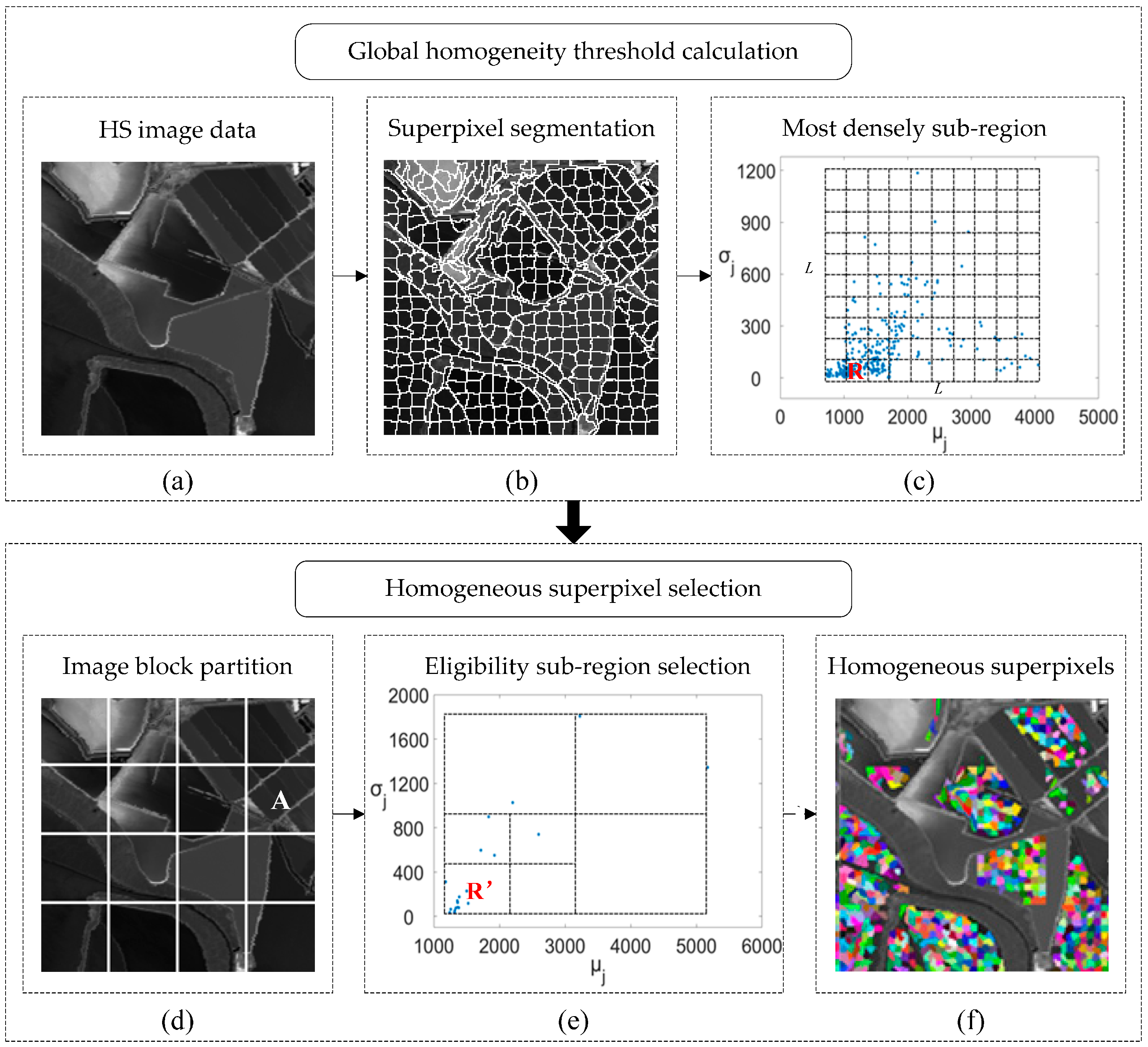
where denotes the pixels belonging to the superpixel , is the number of these pixels, and represents the mean value of all the spectral bands of pixel . Then, we draw the scatter plot of the mean value versus the standard deviation of all the superpixels in the image. In practice, the homogeneous superpixels contain mainly stationary noise information; in contrast, the inhomogeneous superpixels generally contain abundant image structures, which results in larger variations of their local statistics. Therefore, the points of homogeneous superpixels will cluster together tightly in the scatter plot, whereas the inhomogeneous superpixels will distribute far away from them. Based on this observation, the framework of the proposed SPHSS algorithm (illustrated in Figure 2) consists of two major steps: (1) calculation of the global homogeneity threshold, and (2) selection of the homogeneous superpixels.
Step 1: Partition the scatter plot plane into a number of sub-regions, and then find the sub-region that contains the most scatter points, i.e., the most densely sub-region (illustrated as sub-region in Figure 2c). The global homogeneity threshold is calculated as:
where is the number of scatter points in the sub-region .
Step 2: To avoid the selected superpixels having similar mean values, we first partition the whole image into a number of blocks. For any image block , shown in Figure 2d, we draw the scatter plot of the mean value versus the standard deviation of all the superpixels in this block, and then calculate the homogeneity parameter similar to Equation (16) as follows:
where is the number of generated superpixels in the image block . If the homogeneity parameter is no larger than the global homogeneity threshold , all of the superpixels in image block are considered as homogenous superpixels; otherwise, split the scatter plot plane into four sub-regions and find the most dense sub-region, and then calculate the corresponding homogeneity parameter and compare with . Repeat this procedure until the sub-region whose homogeneity parameter satisfies the global homogeneity threshold is found, or until it is determined that there is no homogeneous superpixel in the image block . As illustrated in Figure 2e, when the homogeneity parameter of sub-region meets the requirement of the global homogeneity threshold, the superpixels whose corresponding scatter points located in the sub-region are selected as the homogeneous superpixels. Similar to the homogeneous superpixel selection process for the image block , we then deal with the rest image blocks and find all of the homogeneous superpixels in the whole image.
3.3. Approximation of SD and SI Noise Variances
After the homogeneous superpixels are selected in the HS image, we apply the MLR model to remove the between-band and within-band correlations in homogeneous superpixels, where the remaining unexplained residuals are considered as the mixed noise.
To deal with the mixed noise in band of a HS image, the image data in bands , , and are used. For the observed image pixel within a homogeneous superpixel, its predicted value is computed as follows:
where , , , and are the regression coefficients, and denotes a spatial neighbor pixel of within the same homogeneous superpixel. In the proposed method, the pixel is selected by searching the eight spatial neighbor pixels sequentially and choosing one neighbor pixel that belongs to the same superpixel of . The computation time for this process is reasonable because only one spatial neighbor pixel is required, so that the first searched neighbor pixel is likely to be an eligible one, except for the boundaries of superpixels. Note that, as a special case, when calculating the predicted value for a pixel in the first or last band of a HS image, only one spectral neighbor band and one spatial neighbor pixel are utilized for the de-correlation process. Based on the predicted value computed by Equation (18), the residual is calculated as:
We use the unbiased estimate of the variance of residuals in the homogeneous superpixel to approximate the mixed noise variance:
where is the number of pixels in the homogeneous superpixel, and degrees of freedom are reduced from to as four parameters are used in the regression.
After mixed noise variances of the all selected homogeneous superpixels are estimated, we exploit the SPE approach to calculate the variances of the SD and SI noise. According to Equation (5), for a particular band , the scatter points will cluster along a straight line (as illustrated in Figure 3), whose intercept and slope are equal to and , respectively. To fit the scatter points more accurately, we apply the least squares linear fitting (LSLF) in the proposed method, where the red line represents the fitting results in Figure 3.
4. Experimental Results and Discussion
In the experiment part, we evaluate the performance of the proposed mixed noise estimation method by using both synthetic and real AVIRIS images. In Section 4.1, the descriptions of the experimental HS images are first introduced, and then the quantitative evaluation metrics are defined. In Section 4.2, the performance of the SSA is evaluated, where the parameter setting is also discussed. In Section 4.3, the accuracy of the proposed FSSMNE is first evaluated with the synthetic HS images in various noise conditions, and then the robustness of our method is verified on real AVIRIS data with different complex image textures.
4.1. Experimental Images and Quantitative Evaluation Metrics
4.1.1. Synthetic and Real HS Images
In order to generate synthetic HS images, five spectra representing different Earth objects are extracted from the real AVIRIS images (as shown in Figure 4). The synthetic HS image is simulated by using the first 90 spectral bands of the extracted spectra, where Figure 5a shows typical example of the 50th band with the spatial size .
In experiments with real HS images, we exploit the AVIRIS image data, which has been widely used for various applications [29,30]. The AVIRIS measures radiance through 224 contiguous channels at 10 nm intervals with four spectrometers: A (bands 1–32, spectral range of 400–700 nm), B (bands 33–96, 700–1300 nm), C (bands 97–160, 1300–1900 nm), and D (bands 161–224, 1900–2500 nm). The utilized AVIRIS image, acquired over Moffett Field, is a radiance data set with 16-bit radiometric resolution [31]. To evaluate the robustness of the proposed noise estimation method on HS images with different complex land covers, two sub-images with the spatial size are cut from an AVIRIS image, namely Date Set 1 and Data Set 2, respectively. Therefore, the noise levels of the two data sets are treated the same. Figure 5b,c show the 50th band of the two data sets, where the image scene of Data Set 1 is relatively simple, while Data Set 2 contains much more textures. Note that in the experimental AVIRIS images, several spectral bands have extremely poor image qualities. They are not mainly caused by random noise but by read-out errors of the detectors or weak signal energy acquired. Similar to the literature [20,32], we remove these spectral bands before using the real HS data in our experiments. After discarding bands 1–10 and 95–130 from Data Sets 1 and 2, we obtain a spectral dimensionality of 178.
4.1.2. Quantitative Evaluation Metrics
In experiments with the synthetic HS image, mixed noise with various noise levels are simulated according to the noise model in Equations (1)–(5). To set the values of the two noise parameters and in band , we use the metric signal-to-noise ratio (SNR) [33] to measure the mixed noise levels as follows:
In addition, a new metric is defined to calculate the SD-to-SI noise ratio (SDSINR) as:
To quantitatively evaluate the performances of the noise estimation methods in experiments with synthetic images, we adopt the relative-mean-square-error (RMSE) of the noise estimates, which are calculated as follows:
where , and , are the estimates and true values of SD and SI noise for the band , respectively. and denote the estimation errors in the th band, and and are the errors averaged over all of the spectral bands.
In experiments with real AVIRIS images, we use the Euclidean distance to quantitatively evaluate the robustness of the methods when HS images have different complexities, where the distances of noise estimates between Data Sets 1 and 2 are calculated as:
where , , and are the estimates of SD noise variance, SI noise variance, and SNR for the band in Data Set 1; , , and are the corresponding estimates for the band in Data Set 2. , and denote the Euclidean distances of the corresponding estimates between Data Sets 1 and 2, which are averaged over all of the utilized spectral bands for comparison.
4.2. Performance of the SSA
The superpixel-generating process is a crucial pre-step in the proposed noise estimation method. In the SSA, the parameter is important for the frequency-based spectral distance as it decides the similarity of the original and the reconstructed spectral signatures. We first investigate the selection of the parameter by using the five spectra in Figure 4 with different parameter values: , where the reconstruction results are shown in Figure 6. From the figure we can observe that the reconstructed spectral curves become more similar to the original curves as the value of parameter increases, so that a larger parameter value is helpful to keep the inherent characteristics of the original spectral signatures. However, a larger may increase the computation time of the superpixel generating process; to make it worse, it will be more sensitive to the image noise. To balance the performance and the computation complexity, we set the parameter in all experiments of this paper. Another parameter in the SSA is introduced to weigh the relative importance between spectral similarity and spatial proximity. When is too small, the spectral similarity weighs more than the spatial similarity and the resulting superpixels are quite irregular in shape, which is adverse to the formation of an interpretable image region and the extraction of locally relevant features. On the other hand, when is too large, the generated superpixels will not adhere adequately to the local image structures. The suggested value for parameter lies between 0.05 and 0.2, and we set in all experiments reported in this paper.
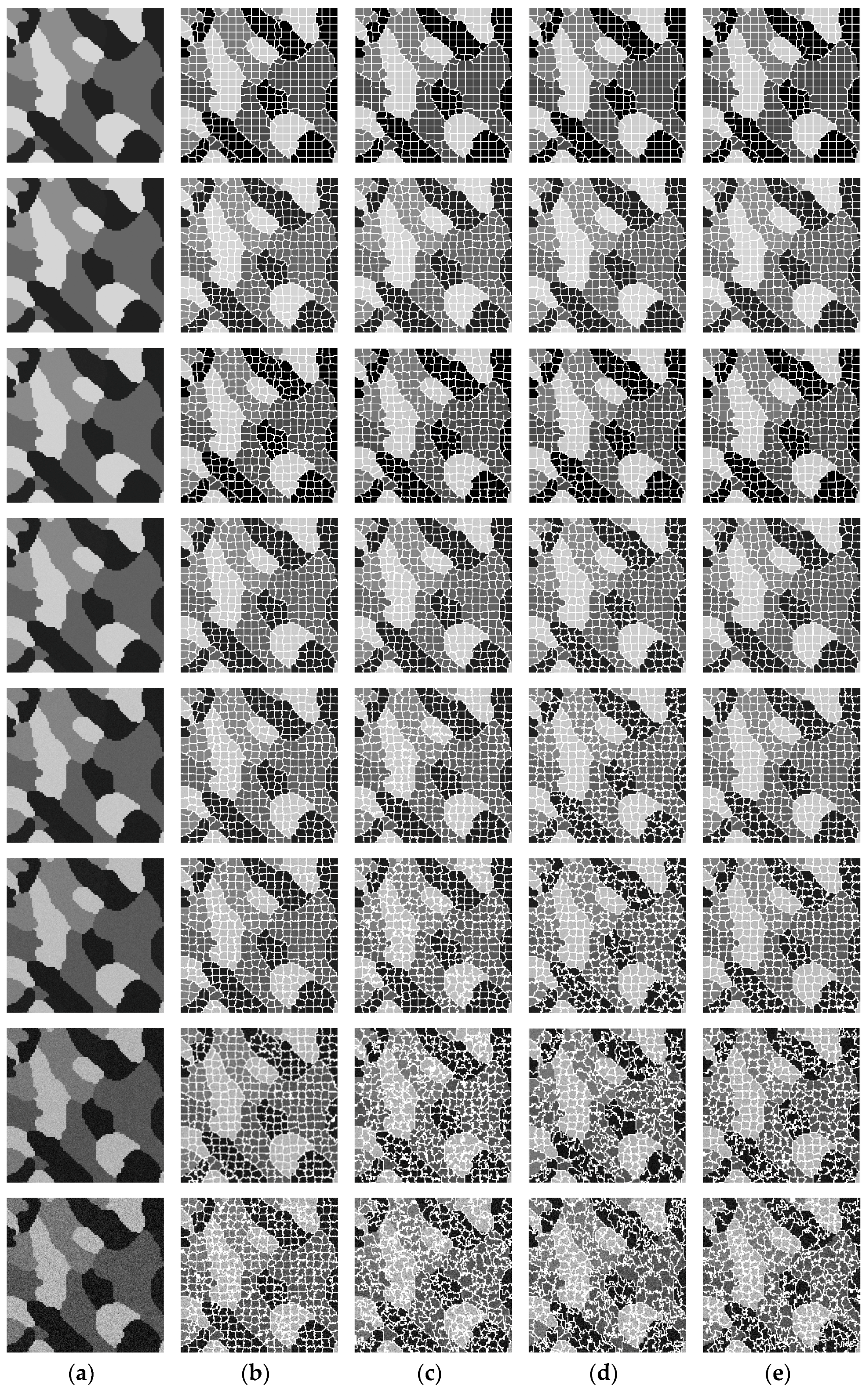
To accurately approximate the noise parameters from HS images with diverse noise levels, the superpixel-generating algorithm is required to be robust to the noise. To evaluate the noise robustness of the superpixel-generating algorithms, the simulated mixed noise with and are added to the synthetic HS image. Superpixels are then generated by using SSA and other three compared algorithms, including SLIC and two modified superpixel-generating algorithms. SLIC is a widely used superpixel-generating algorithm for natural images, which exploits the Euclidean distance of the pixel intensities to cluster the similar image pixels. For a more comprehensive and fair comparison, we modify SLIC by using two widely applied spectral similarities—spectral angle mapping (SAM) [34] and spectral correlation mapper (SCM) [35] to cluster similar pixels in HS images and then produce superpixels, namely SLIC-SAM and SLIC-SCM, respectively. Superpixel segmentation results with the four considered algorithms are displayed in Figure 7. As shown, the superpixels generated by the four algorithms have marginal differences with small noise levels. However, with the increase of the image noise levels, the performances of SLIC, SLIC-SAM, and SLIC-SCM decrease considerably; in contrast, the proposed SSA can still adhere to the local image structures. This advantage results mainly from the benefits of defining the spectral similarity in frequency domain, which significantly reduces the impact of the image noise. To quantitatively evaluate the performance of the compared superpixel-generating algorithms, the measure boundary recall [36], widely used as an indicator of the boundary adherence ability, is also adopted in this experiment. The boundary recall measures what fraction of the ground truth image structures fall within at least two pixels of a superpixel boundary. A higher boundary recall means that fewer image structures are missed, and therefore indicates a better performance of the superpixel-generating algorithm. The boundary recall of each algorithm is plotted in Figure 8 for increasing SNR values. From this figure we can see that with low noise levels, all of the compared algorithms produce accurate superpixel segmentation results; when the image noise level increases, the proposed SSA performs much better than the other three algorithms. We have also done some experiments with different values, and the results are similar to those in Figure 7 and Figure 8. The experimental results in this section conclude that the proposed SSA is more robust than the compared superpixel-generating algorithms in more severe noise conditions.
4.3. Performance of the FSSMNE Noise Estimation Method
To quantitatively evaluate the performance of the proposed FSSMNE noise estimation method, we design three numerical experiments with the synthetic HS image: (1) evaluate the accuracy of the FSSMNE and other three noise estimation methods with fixed and values; (2) evaluate the accuracy of the FSSMNE with various noise levels; and (3) evaluate the accuracy of the FSSMNE with various ratios of SD and SI noise. Furthermore, by using the real AVIRIS images, we evaluate the robustness of the proposed FSSMNE and other three compared methods when HS images have different complex land covers.
4.3.1. Experiments on the Synthetic HS Image
(1) Accuracy evaluation of FSSMNE and compared methods. In this experiment, SD and SI noise are added to the synthetic HS image with and , where the true values of parameters and can be obtained according to Equations (21) and (22). The proposed FSSMNE is compared with other three state-of-the-art noise estimation methods, including HS noise parameter estimation (HSNPE) [20], signal-dependent noise estimation (SDNE) [24], and intensity-variance homogeneity classification-based noise estimation (IVHCNE) [25].
First, we adopt the proposed SSA to segment the synthetic image into superpixels with initial size , and then the most homogeneous superpixels are selected with SPHSS, where the parameters are set as and based on the estimation performance. The selected homogeneous superpixels for the synthetic image are illustrated in Figure 9a with different colours. Note that in the proposed noise estimation method, there is no need to locate all of the homogeneous superpixels, but it is a must to make sure that the selected superpixels are strictly homogeneous.
The proposed FSSMNE and the compared noise estimation methods are applied to the synthetic HS image data. Estimates of SD and SI noise variances obtained by the considered methods are presented in Figure 10; the RMSEs of the noise estimation results are calculated according to Equations (23) and (24) and recorded in Table 1. The curves in Figure 10 demonstrate that the FSSMNE provides more accurate noise estimation results than the compared methods in most spectral bands. Considering the quantitative results presented in Table 1, we can further confirm that the FSSMNE outperforms the other three compared methods on the synthetic HS image. The HSNPE produces less accurate estimates mainly due to the fact that this method only exploits the spectral information of the HS image data but ignores the spatial information. In SDNE and IVHCNE, the homogeneous image regions are first selected with the spatial information, and the accuracy of these two noise estimation methods mainly depends on the performances of their respective homogeneous image region selection approaches. From estimation results displayed in Figure 10 and Table 1, we find that IVHCNE performs much better than SDNE but is still not in competition with our noise estimation method. The main reason is that the homogeneous image regions are detected on each individual band of the HS data in IVHCNE and SDNE, while in the proposed FSSMNE, the spectral and spatial information are effectively exploited to generate homogeneous superpixels.
(2) Accuracy evaluation of FSSMNE with various noise levels. In the previous experiment, the proposed FSSMNE has been demonstrated to be well-performing on the synthetic HS image with a fixed noise level. In this experiment, we evaluate the performance of the proposed FSSMNE on synthetic HS images with various noise levels. Mixed noise is added to the synthetic HS image with and to test the noise estimation accuracy of the FSSMNE. The two quantitative metrics and are calculated and recorded in Table 2. From the experimental results in the table, we can observe that the proposed FSSMNE provides accurate SD and SI noise estimates when the image noise levels vary in quite a big range. Particularly, when the value is larger than 20, the noise estimation errors are extremely small.
(3) Accuracy evaluation of FSSMNE with various ratios of SD and SI noise. We simply assumed that the contribution of SD and SI noise is the same in the first two experiments. In order to evaluate the proposed noise estimation method comprehensively, we add mixed noise to the synthetic HS image with and various values: . The SD and SI noise estimation errors with the proposed FSSMNE are recoded in Table 3. It is observed that our method performs well when the ratio of SD and SI noise varies from 1/4 to 4. Particularly, the FSSMNE produces more accurate SD noise estimates when the weight of the SD noise component increases; the same applies to the SI noise estimation.
4.3.2. Experiments on AVIRIS Images
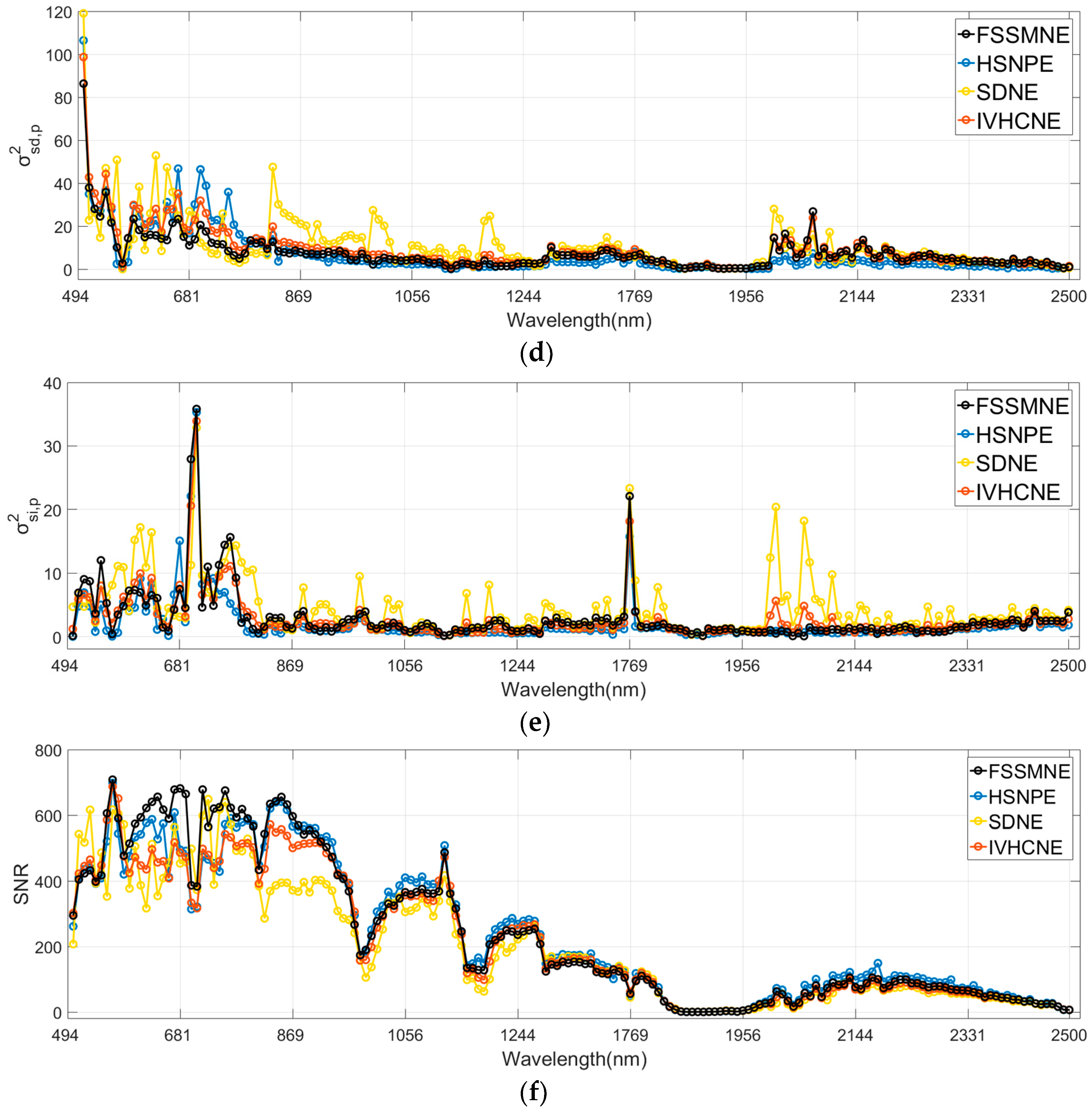
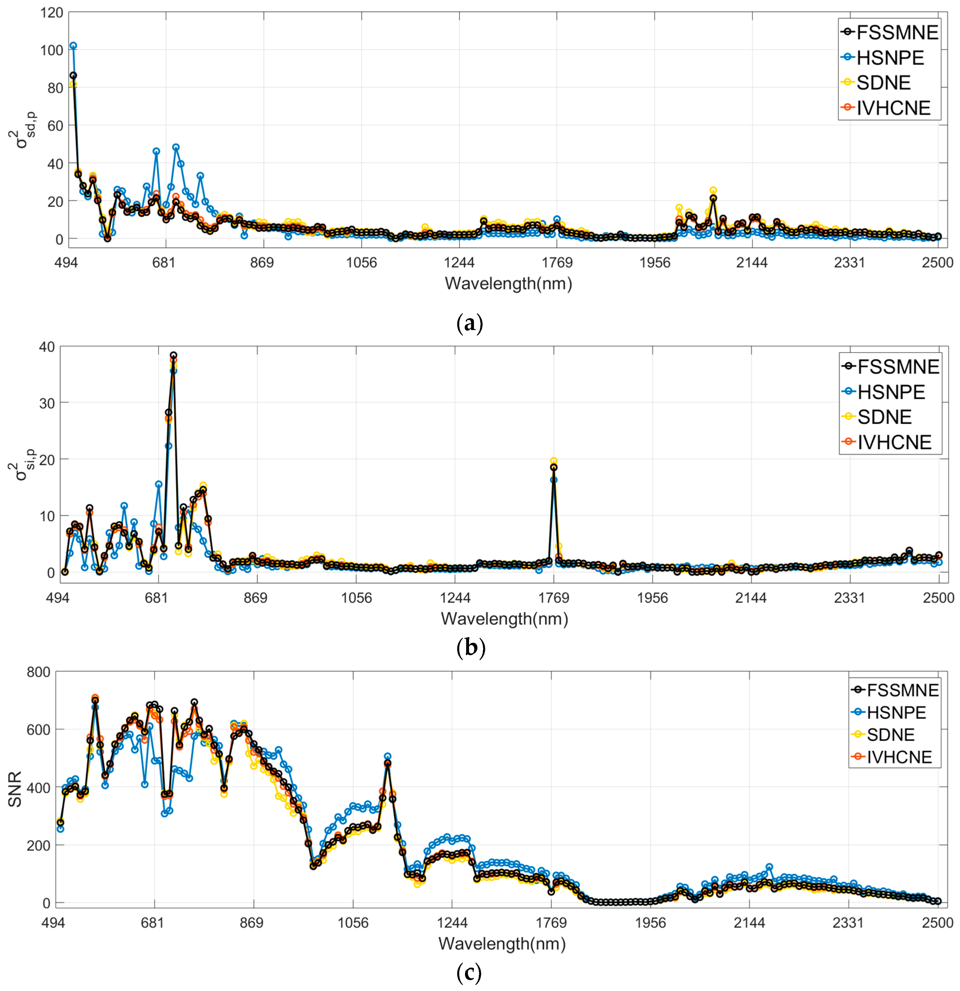
In this experiment, we evaluate the robustness of the noise estimation methods on real AVIRIS images with different complex land covers. For this purpose, the simply textured Data Set 1 and the highly textured Data Set 2 are utilized. First, the homogeneous superpixels are located in the two data sets and the results are showed in Figure 9b,c. It is observed from the figures that the proposed method can accurately detect homogeneous superpixels for both simple and complex images, which paves the way for the subsequent noise parameter estimation. We use estimates of SD noise variance, SI noise variance, and SNR to evaluate the performance of the noise estimation methods, where the estimation results of the considered methods (FSSMNE, HSNPE, SDNE, and IVHCNE) are presented in Figure 11, and the averaged Euclidean distances of noise estimates between Data Sets 1 and 2 are calculated according to Equations (25)–(27) and recorded in Table 4. From Figure 11a–c, we can see that FSSMNE, SDNE, and IVHCNE produce similar noise estimation results with the simply textured Data Set 1. However, when dealing with the richly textured Data Set 2, the estimation results of SDNE and IVHCNE are significantly deviated from those obtained with Data Set 1. Leveraging the advantages of the accurate superpixel segmentation, the proposed FSSMNE produces consistent noise estimation results with the two data sets, where the quantitative results in Table 4 further demonstrate that our method is more robust than SDNE and IVHCNE on HS images with different complex land covers. Regarding HSNPE, the method produces more consistent noise estimates than FSSMNE with the Data Sets 1 and 2; this is mainly because HSNPE only exploits the spectral information to approximate the noise variances. However, the lack of spatial information may reduce the accuracy of the method, which has been demonstrated in the experiments with synthetic images. In addition, Figure 11a–c shows that the noise estimation results of HSNPE are quite different from those obtained by the other three methods with simply textured images, which also implies that the HSNPE is less accurate than the compared methods. It’s worth noting that there are some noise spikes existing in the noise estimation results, especially in the SI noise variance estimates. As shown in Figure 11b, two obvious spikes are existing in the graph. The first spike is presented at 700 nm, mainly because it is the border of spectrometers A and B; the second spike is located near 1770 nm and is related to the detector problems, which has been discussed in detail in [13]. Regarding the SNR estimates in Figure 11c, we can see that the SNR values of the image data produced by spectrometers A and B are much higher than those obtained by spectrometers C and D. Particularly, in the water absorption bands (1850–1980 nm), the SNR values are extremely small. Note that in the noise estimation results of the proposed method, the value of the SD noise variance varies from 0–10 in most bands and the SI noise variance lies in the range 0–5, which further proves it is appropriate to model the noise as a mixture of the SD and SI noise components in AVIRIS images.
5. Conclusions
This paper proposes a hyperspectral image segmentation method for automated SD and SI mixed noise estimation. In contrast with the conventional rectangular-block division algorithms, the images are segmented into superpixels that exhibit better adherence to the local image structure, thus generating a division into small regions that are more likely to be homogeneous regions. Moreover, a novel frequency-based spectral similarity measure is proposed to make the SSA more insensitive to the image noise. An improved homogeneous superpixel selection algorithm and the MLR-based noise parameter estimation approach boost the performance of the proposed FSSMNE to accurately approximate the mixed noise parameters with different image complexities and various noise conditions. Experimental results with the synthetic HS image demonstrate that the proposed FSSMNE outperforms the compared state-of-the-art noise estimation methods. Furthermore, experiments with real HS data verify the robustness of the FSSMNE when the images have different complex land covers. It is worth noting that the proposed superpixel segmentation algorithm can be used as the first step of many noise estimation methods with diverse noise types. However, the use of the spectral information and the transformation process to the frequency domain may increase the complexity of the method. Improvements to the efficiency of the proposed method without decreasing its accuracy and robustness will be studied in future works.
Acknowledgments
This work was supported by the National Natural Science Foundation of China under Grant No. 61673220.
Author Contributions
Peng Fu conceived of and designed the experiments. Peng Fu and Xin Sun processed and analyzed the data. Peng Fu and Quansen Sun wrote the paper.
Conflicts of Interest
The authors declare no conflict of interest.
References
- Gao, L.; Zhao, B.; Jia, X.; Liao, W.; Zhang, B. Optimized kernel minimum noise fraction transformation for hyperspectral image classification. Remote Sens. 2017, 9, 548. [Google Scholar] [CrossRef]
- Li, J.; Yuan, Q.; Shen, H.; Zhang, L. Noise removal from hyperspectral image with joint spectral-spatial distributed sparse representation. IEEE Trans. Geosci. Remote Sens. 2016, 54, 5425–5439. [Google Scholar] [CrossRef]
- He, W.; Zhang, H.; Zhang, L.; Shen, H. Hyperspectral image denoising via noise-adjusted iterative low-rank matrix approximation. IEEE J. Sel. Top. Appl. Earth Obs. Remote Sens. 2015, 8, 3050–3061. [Google Scholar] [CrossRef]
- Tang, Z.; Fu, G.; Chen, J.; Zhang, L. A unified model of noise estimation, band rejection, and de-noising for hyperspectral images. Int. J. Remote Sens. 2016, 37, 1319–1348. [Google Scholar] [CrossRef]
- Jia, S.; Tang, G.; Zhu, J.; Li, Q. A novel ranking-based clustering approach for hyperspectral band selection. IEEE Trans. Geosci. Remote Sens. 2016, 54, 88–102. [Google Scholar] [CrossRef]
- Yang, M.D.; Huang, K.S.; Yang, Y.F.; Lu, L.Y.; Feng, Z.Y.; Tsai, H.P. Hyperspectral image classification using fast and adaptive bidimensional empirical mode decomposition with minimum noise fraction. IEEE Geosci. Remote Sens. Lett. 2016, 13, 1950–1954. [Google Scholar] [CrossRef]
- Zheng, X.; Yuan, Y.; Lu, X. A target detection method for hyperspectral image based on mixture noise model. Neurocomputing 2016, 216, 331–341. [Google Scholar] [CrossRef]
- Ertürk, A.; Plaza, A. Informative change detection by unmixing for hyperspectral images. IEEE Geosci. Remote Sens. Lett. 2015, 12, 1252–1256. [Google Scholar] [CrossRef]
- Fu, P.; Li, C.; Xia, Y.; Ji, Z.; Sun, Q.; Cai, W.; Feng, D.D. Adaptive noise estimation from highly textured hyperspectral images. Appl. Opt. 2014, 53, 7059–7071. [Google Scholar] [CrossRef] [PubMed]
- Chen, Y.; Huang, T.; Zhao, X.; Deng, L.; Huang, J. Stripe noise removal of remote sensing images by total variation regularization and group sparsity constraint. Remote Sens. 2017, 9, 559. [Google Scholar] [CrossRef]
- Meola, J.; Eismann, M.T.; Moses, R.L.; Ash, J.N. Modeling and estimation of signal-dependent noise in hyperspectral imagery. Appl. Opt. 2011, 50, 3829–3846. [Google Scholar] [CrossRef] [PubMed]
- Fujimoto, N.; Takahashi, Y.; Moriyama, T.; Shimada, M.; Wakabayashi, H.; Nakatani, Y.; Obayani, S. Evaluation of SPOT HRV image data received in Japan. In Proceedings of the International Geoscience and Remote Sensing Symposium, Vancouver, BC, Canada, 10–14 July 1989; pp. 463–466. [Google Scholar]
- Gao, B. An operational method for estimating signal to noise ratios from data acquired with imaging spectrometers. Remote Sens. Environ. 1993, 43, 23–33. [Google Scholar] [CrossRef]
- Corner, B.R.; Narayanan, R.M.; Reichenbach, S.E. Noise estimation in remote sensing imagery using data masking. Int. J. Remote Sens. 2003, 24, 689–702. [Google Scholar] [CrossRef]
- Qin, B.; Hong, B.; Zhang, Z.; Yang, X.; Li, Z. A generally applicable noise-estimating method for remote sensing images. Remote Sens. Lett. 2014, 5, 481–490. [Google Scholar] [CrossRef]
- Fu, P.; Sun, Q.; Ji, Z.; Chen, Q. A new method for noise estimation in single-band remote sensing images. In Proceedings of the IEEE International Conference on Fuzzy Systems and Knowledge Discovery, Chongqing, China, 29–31 May 2012; pp. 1664–1668. [Google Scholar]
- Roger, R.E.; Arnold, J.F. Reliably estimating the noise in AVIRIS hyperspectral images. Int. J. Remote Sens. 1996, 17, 1951–1962. [Google Scholar] [CrossRef]
- Gao, L.; Zhang, B.; Zhang, X.; Zhang, W.; Tong, Q. A new operational method for estimating noise in hyperspectral images. IEEE Geosci. Remote Sens. Lett. 2008, 5, 83–87. [Google Scholar] [CrossRef]
- Martin-Herrero, J. Comments on “a new operational method for estimating noise in hyperspectral images”. IEEE Geosci. Remote Sens. Lett. 2008, 5, 705–709. [Google Scholar] [CrossRef]
- Acito, N.; Diani, M.; Corsini, G. Signal-dependent noise modeling and model parameter estimation in hyperspectral images. IEEE Trans. Geosci. Remote Sens. 2011, 49, 2957–2971. [Google Scholar] [CrossRef]
- Sun, L. Signal-dependent noise parameter estimation of hyperspectral remote sensing images. Spectrosc. Lett. 2015, 48, 717–725. [Google Scholar] [CrossRef]
- Uss, M.L.; Vozel, B.; Lukin, V.V.; Chehdi, K. Local signal-dependent noise variance estimation from hyperspectral textural images. IEEE J. Sel. Top. Signal Process. 2011, 5, 469–486. [Google Scholar] [CrossRef]
- Lee, J.S.; Hoppel, K. Noise Modeling and estimation of remotely-sensed images. In Proceedings of the IEEE International Geoscience and Remote Sensing Symposium, Vancouver, BC, Canada, 10–14 July 1989; pp. 1005–1008. [Google Scholar]
- Alparone, L.; Selva, M.; Aiazzi, B.; Baronti, S.; Butera, F.; Chiarantini, L. Signal-dependent noise modelling and estimation of new-generation imaging spectrometers. In Proceedings of the IEEE Workshop on Hyperspectral Image & Signal Processing: Evolution in Remote Sensing, Grenoble, France, 26–28 August 2009; pp. 1–4. [Google Scholar]
- Rakhshanfar, M.; Amer, M.A. Estimation of Gaussian, Poissonian-Gaussian, and processed visual noise and its level function. IEEE Trans. Image Process. 2016, 25, 4172–4185. [Google Scholar] [CrossRef] [PubMed]
- Foi, A.; Trimeche, M.; Katkovnik, V.; Egiazarian, K. Practical Poissonian-Gaussian noise modeling and fitting for single-image raw-data. IEEE Trans. Image Process. 2008, 17, 1737–1754. [Google Scholar] [CrossRef] [PubMed]
- Achanta, R.; Shaji, A.; Smith, K.; Lucchi, A.; Fua, P.; Süsstrunk, S. SLIC superpixels compared to state-of-the-art superpixel methods. IEEE Trans. Pattern Anal. Mach. Intell. 2012, 34, 2274–2282. [Google Scholar] [CrossRef] [PubMed]
- Wang, K.; Yong, B. Application of the frequency spectrum to spectral similarity measures. Remote Sens. 2016, 8, 344. [Google Scholar] [CrossRef]
- Yang, J.; Zhao, Y.; Yi, C.; Chan, J.C.W. No-reference hyperspectral image quality assessment via quality-sensitive features learning. Remote Sens. 2017, 9, 305. [Google Scholar] [CrossRef]
- He, T.; Liang, S.; Wang, D.; Shi, Q.; Goulden, M.L. Estimation of high-resolution land surface net shortwave radiation from AVIRIS data: Algorithm development and preliminary results. Remote Sens. Environ. 2015, 167, 20–30. [Google Scholar] [CrossRef]
- AVIRIS—Airborne Visible/Infrared Imaging Spectrometer—Data. Available online: http://aviris.jpl.nasa.gov/data/free_data.html (accessed on 6 November 2008).
- Mahmood, A.; Robin, A.; Sears, M. Modified residual method for the estimation of noise in hyperspectral images. IEEE Trans. Image Process. 2017, 55, 1451–1460. [Google Scholar] [CrossRef]
- Curran, P.J.; Dungan, J.L. Estimation of signal-to-noise: A new procedure applied to AVIRIS data. IEEE Trans. Geosci. Remote Sens. 1989, 27, 620–628. [Google Scholar] [CrossRef]
- Jiao, H.; Zhong, Y.; Zhang, L. Artificial DNA computing-based spectral encoding and matching algorithm for hyperspectral remote sensing data. IEEE Trans. Geosci. Remote Sens. 2012, 50, 4085–4104. [Google Scholar] [CrossRef]
- Deborah, H.; Richard, N.; Hardeberg, J.Y. A comprehensive evaluation of spectral distance functions and metrics for hyperspectral image processing. IEEE J. Sel. Top. Appl. Earth Obs. Remote Sens. 2015, 8, 3224–3234. [Google Scholar] [CrossRef]
- Levinshtein, A.; Stere, A.; Kutulakos, K.; Fleet, D.; Dickinson, S.; Siddiqi, K. Turbopixels: Fast superpixels using geometric flows. IEEE Trans. Pattern Anal. Mach. Intell. 2009, 31, 2290–2297. [Google Scholar] [CrossRef] [PubMed]
Figure 1.
Illustration of the frequency spectrum transformation and its reconstruction under noise corruption. (a) The original and noisy spectral curves; (b) the frequency transformation results of the original and noisy spectral signatures; (c) the reconstruction results of the original and noisy spectra.
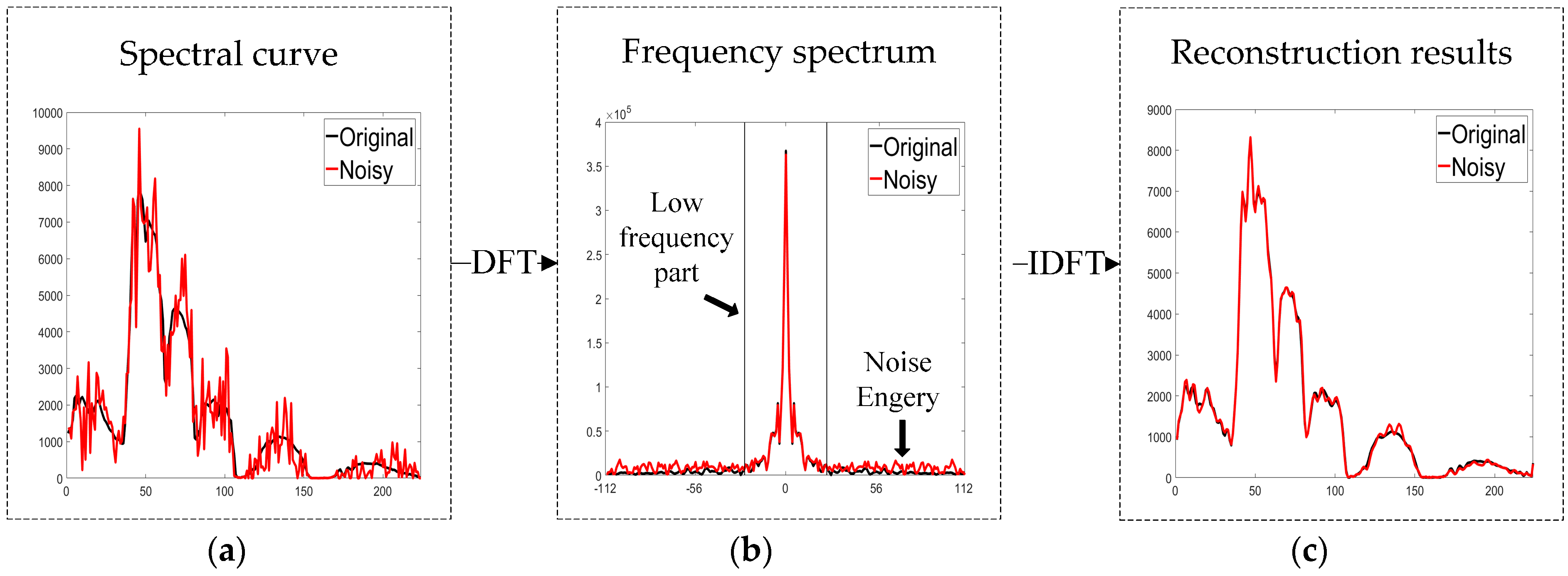
Figure 2.
The processing flow of the proposed automated scatter-plot-based homogeneous superpixel selection algorithm. (a) The input HS image data (one spatial band); (b) the superpixel segmentation result; (c) the most dense sub-region in the scatter plot; (d) the image block partition result; (e) the eligibility sub-region in the scatter plot of block ; (f) the homogeneous superpixels selection results of the whole image.

Figure 3.
Illustration of the scatter points and line fitting in the process of calculating signal-dependent (SD) and signal-independent (SI) noise variances.
Figure 3.
Illustration of the scatter points and line fitting in the process of calculating signal-dependent (SD) and signal-independent (SI) noise variances.
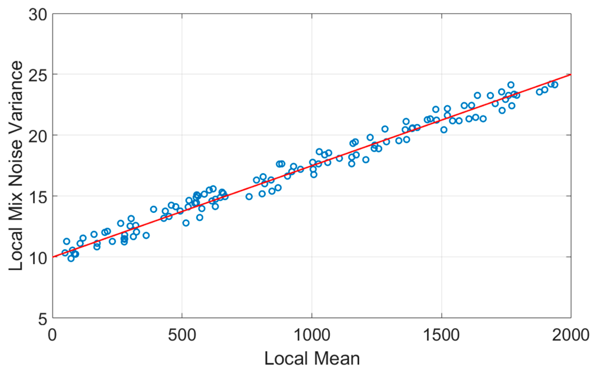
Figure 4.
The five extracted spectra for the synthetic hyperspectral (HS) image simulation (first 90 bands).
Figure 4.
The five extracted spectra for the synthetic hyperspectral (HS) image simulation (first 90 bands).
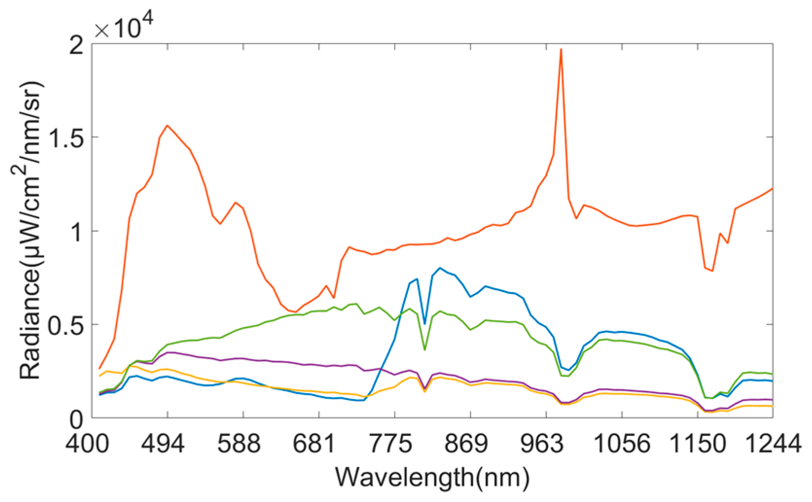
Figure 5.
Synthetic and real HS images utilized in the experiment. (a) The 50th band of the synthetic HS image with camouflage pattern; (b) the 50th band of the real HS image with simple textures; (c) the 50th band of the real HS image with complex textures.
Figure 5.
Synthetic and real HS images utilized in the experiment. (a) The 50th band of the synthetic HS image with camouflage pattern; (b) the 50th band of the real HS image with simple textures; (c) the 50th band of the real HS image with complex textures.
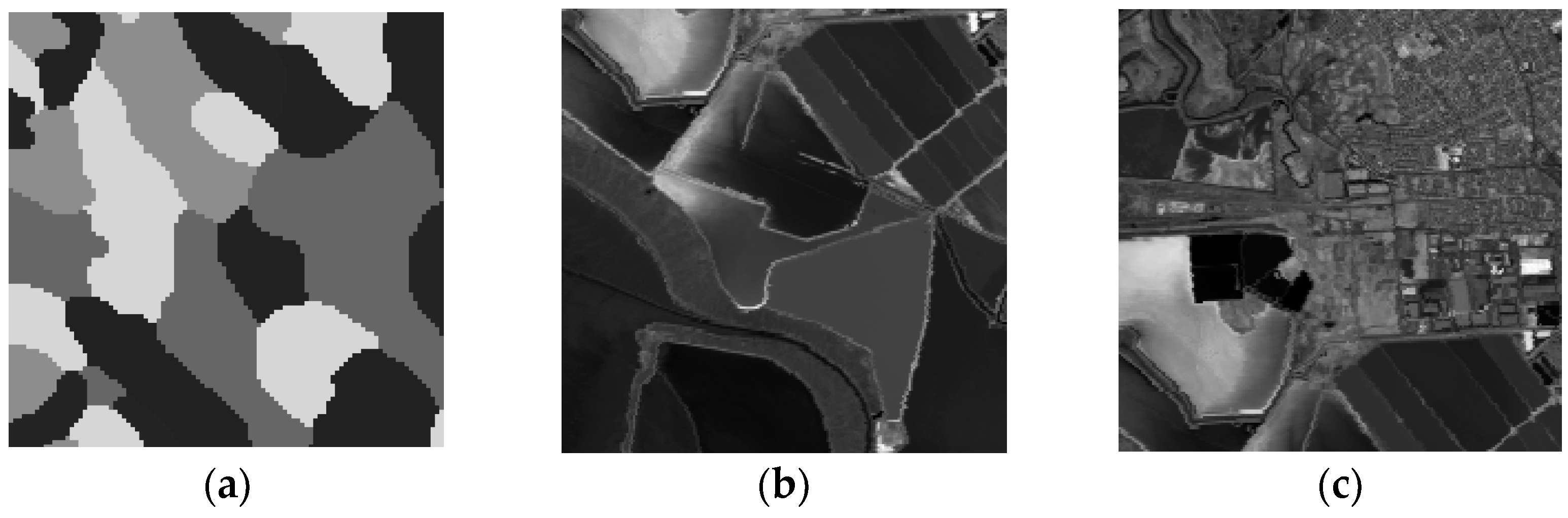
Figure 6.
Reconstructed spectral signatures with different values of parameter . (a) ; (b) ; (c) ; (d) ; (e) ; (f) .
Figure 6.
Reconstructed spectral signatures with different values of parameter . (a) ; (b) ; (c) ; (d) ; (e) ; (f) .

Figure 7.
Superpixels generated by SSA, SLIC, SLIC-SAM, and SLIC-SCM from the synthetic HS image at various noise levels. (a) Original and noisy images with and from row 1 to the row 8; (b) superpixels generated by SSA from the corresponding images; (c) superpixels generated by SLIC from the corresponding images; (d) superpixels generated by SLIC-SAM from the corresponding images; (e) superpixels generated by SLIC-SCM from the corresponding images. SSA, superpixel segmentation algorithm; SLIC, simple linear iterative clustering; SLIC-SAM, SLIC-spectral angle mapping; SLIC-SCM, SLIC-spectral correlation mapper; SDSINR, SD-to-SI noise ratio.

Figure 8.
Boundary recall values of the superpixels generated by the SSA, SLIC, SLIC-SAM, and SLIC-SCM from synthetic images with various signal-to-noise ratio (SNR) values.
Figure 8.
Boundary recall values of the superpixels generated by the SSA, SLIC, SLIC-SAM, and SLIC-SCM from synthetic images with various signal-to-noise ratio (SNR) values.
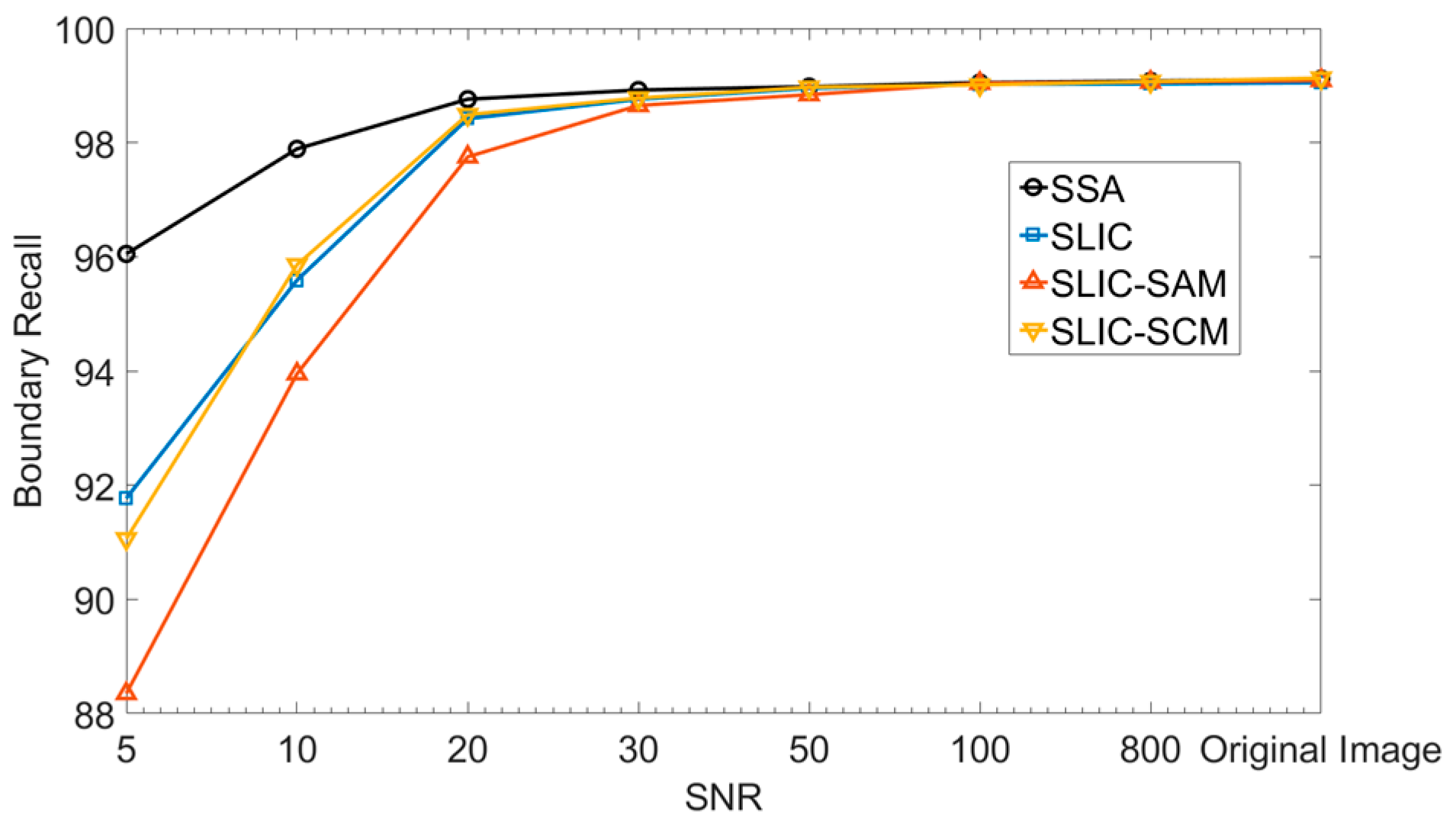
Figure 9.
Homogeneous superpixel selection results with the SPHSS on synthetic and real HS images. (a) The selected homogeneous superpixels in the synthetic image; (b) the selected homogeneous superpixels in the Data Set 1; (c) the selected homogeneous superpixels in the Data Set 2. SPHSS, scatter-plot-based homogenous superpixel selection.
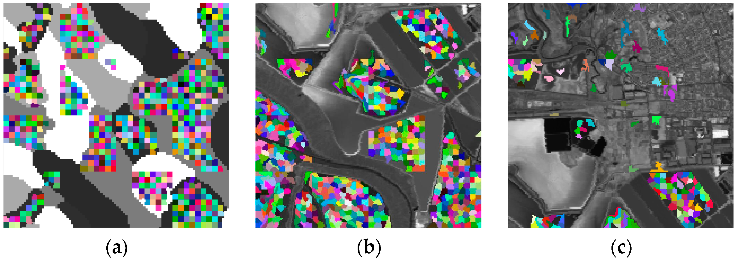
Figure 10.
Noise estimates in each band of the synthetic HS image using the FSSMNE, HSNPE, SDNE, and IVHCNE methods. (a) Estimates of the SD noise variance; (b) estimates of the SI noise variance. FSSMNE, frequency superpixel segmentation-based mixed noise estimation; HSNPE, hyperspectral noise parameter estimation; SDNE, signal-dependent noise estimation; IVHCNE, intensity-variance homogeneity classification-based noise estimation.
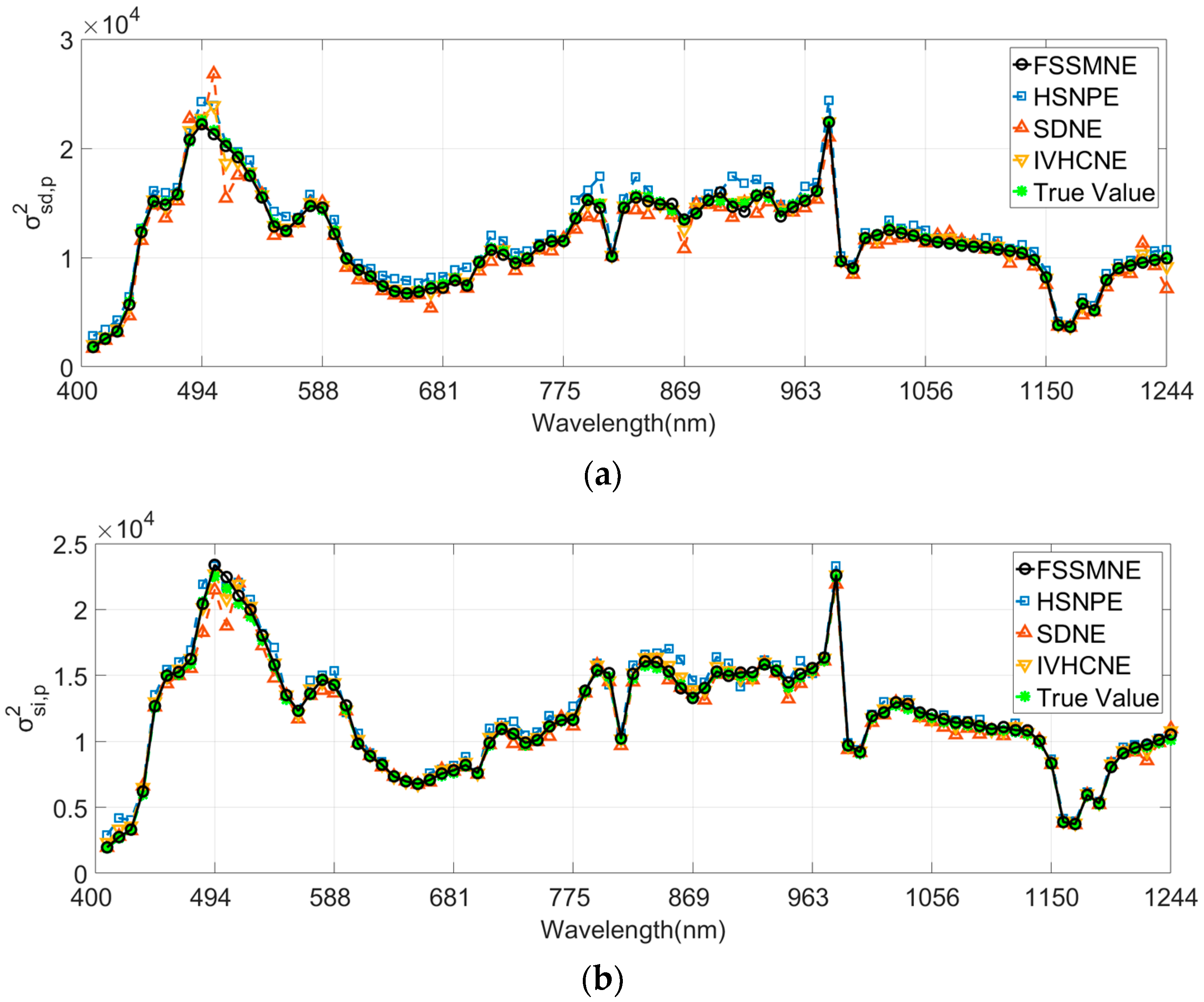
Figure 11.
Noise estimates in each band of the real HS image using the FSSMNE, HSNPE, SDNE, and IVHCNE methods. (a) Estimates of the SD noise variance with Data Set 1; (b) estimates of the SI noise variance with Data Set 1; (c) estimates of the SNR with Data Set 1; (d) estimates of the SD noise variance with Data Set 2; (e) estimates of the SI noise variance with Data Set 2; (f) estimates of the SNR with Data Set 2.


Table 1.
Estimation errors of SD and SI noise on the synthetic HS image with different methods.
| Methods | FSSMNE | HSNPE | SDNE | IVHCNE |
|---|---|---|---|---|
| 8.2 × 10⁻⁴ | 6.8 × 10⁻³ | 6.7 × 10⁻³ | 2.0 × 10⁻³ | |
| 6.2 × 10⁻⁴ | 9.5 × 10⁻³ | 1.6 × 10⁻³ | 9.9 × 10⁻⁴ |
Table 2.
Estimation errors of SD and SI noise on the synthetic HS image with various values.
| 5 | 10 | 20 | 30 | 50 | 100 | 800 | |
|---|---|---|---|---|---|---|---|
| 2.7 × 10⁻² | 7.8 × 10⁻³ | 1.5 × 10⁻³ | 8.2 × 10⁻⁴ | 8.1 × 10⁻⁴ | 8.0 × 10⁻⁴ | 8.0 × 10⁻⁴ | |
| 2.5 × 10⁻² | 6.4 × 10⁻³ | 1.9 × 10⁻³ | 6.2 × 10⁻⁴ | 5.9 × 10⁻⁴ | 5.5 × 10⁻⁴ | 5.3 × 10⁻⁴ |
Table 3.
Estimation errors of SD and SI noise on the synthetic HS image with various values.
| 1/4 | 1/3 | 1/2 | 1 | 2 | 3 | 4 | |
|---|---|---|---|---|---|---|---|
| 2.5 × 10⁻³ | 1.9 × 10⁻³ | 1.4 × 10⁻³ | 8.2 × 10⁻⁴ | 7.4 × 10⁻⁴ | 7.3 × 10⁻⁴ | 5.6 × 10⁻⁴ | |
| 5.1 × 10⁻⁴ | 7.0 × 10⁻⁴ | 7.6 × 10⁻⁴ | 6.2 × 10⁻⁴ | 9.7 × 10⁻⁴ | 1.8 × 10⁻³ | 2.4 × 10⁻³ |
Table 4.
Averaged Euclidean distances of noise estimates between Data Sets 1 and 2 with different methods.
Table 4.
Averaged Euclidean distances of noise estimates between Data Sets 1 and 2 with different methods.
| Methods | FSSMNE | HSNPE | SDNE | IVHCNE |
|---|---|---|---|---|
| 1.545 | 1.302 | 9.242 | 3.710 | |
| 0.770 | 0.409 | 4.045 | 1.209 | |
| 44.612 | 30.716 | 78.234 | 60.301 |
© 2017 by the authors. Licensee MDPI, Basel, Switzerland. This article is an open access article distributed under the terms and conditions of the Creative Commons Attribution (CC BY) license (http://creativecommons.org/licenses/by/4.0/).
Share and Cite
MDPI and ACS Style
Fu, P.; Sun, X.; Sun, Q. Hyperspectral Image Segmentation via Frequency-Based Similarity for Mixed Noise Estimation. Remote Sens. 2017, 9, 1237. https://doi.org/10.3390/rs9121237
AMA Style
Fu P, Sun X, Sun Q. Hyperspectral Image Segmentation via Frequency-Based Similarity for Mixed Noise Estimation. Remote Sensing. 2017; 9(12):1237. https://doi.org/10.3390/rs9121237
Chicago/Turabian StyleFu, Peng, Xin Sun, and Quansen Sun. 2017. "Hyperspectral Image Segmentation via Frequency-Based Similarity for Mixed Noise Estimation" Remote Sensing 9, no. 12: 1237. https://doi.org/10.3390/rs9121237
Note that from the first issue of 2016, this journal uses article numbers instead of page numbers. See further details here.