Article

An Integrated Procedure to Assess the Stability of Coastal Rocky Cliffs: From UAV Close-Range Photogrammetry to Geomechanical Finite Element Modeling

1
DIEF, Department of Engineering ‘Enzo Ferrari’, University of Modena and Reggio Emilia, 41125 Modena, Italy
2
DiSCi, Geography Section, Department of History, Culture and Civilisation, University of Bologne, 40124 Bologne, Italy
3
CNR-IRPI, Istituto Ricerca Protezione Idrogeologica, 70126 Bari, Italy
*
Author to whom correspondence should be addressed.
Remote Sens. 2017, 9(12), 1235; https://doi.org/10.3390/rs9121235
Submission received: 29 September 2017 / Revised: 24 November 2017 / Accepted: 27 November 2017 / Published: 29 November 2017
(This article belongs to the Section Remote Sensing in Geology, Geomorphology and Hydrology)

Abstract

:
The present paper explores the combination of unmanned aerial vehicle (UAV) photogrammetry and three-dimensional geomechanical modeling in the investigation of instability processes of long sectors of coastal rocky cliffs. The need of a reliable and detailed reconstruction of the geometry of the cliff surfaces, beside the geomechanical characterization of the rock materials, could represent a very challenging requirement for sub-vertical coastal cliffs overlooking the sea. Very often, no information could be acquired by alternative surveying methodologies, due to the absence of vantage points, and the fieldwork could pose a risk for personnel. The case study is represented by a 600 m long sea cliff located at Sant’Andrea (Melendugno, Apulia, Italy). The cliff is characterized by a very complex geometrical setting, with a suggestive alternation of 10 to 20 m high vertical walls, with frequent caves, arches and rock-stacks. Initially, the rocky cliff surface was reconstructed at very fine spatial resolution from the combination of nadir and oblique images acquired by unmanned aerial vehicles. Successively, a limited area has been selected for further investigation. In particular, data refinement/decimation procedure has been assessed to find a convenient three-dimensional model to be used in the finite element geomechanical modeling without loss of information on the surface complexity. Finally, to test integrated procedure, the potential modes of failure of such sector of the investigated cliff were achieved. Results indicate that the most likely failure mechanism along the sea cliff examined is represented by the possible propagation of shear fractures or tensile failures along concave cliff portions or over-hanging due to previous collapses or erosion of the underlying rock volumes. The proposed approach to the investigation of coastal cliff stability has proven to be a possible and flexible tool in the rapid and highly-automated investigation of hazards to slope failure in coastal areas.

Graphical Abstract

1. Introduction

The instability processes of sea rocky cliffs pose a significant hazard to communities and infrastructures located along the coastline. In particular, for those areas highly devoted to touristic and recreational activities, the occurrence of rock falls and slope failures can threaten the safety of people and compromise the local economies related to the touristic activities. Nowadays, the diagnosis of the rock surface of sea cliffs could be developed by means of monitoring operations based on advanced surveying methodologies. Among these, aerial or terrestrial (TLS) LiDAR, close range photogrammetry, field surveys with total station and compass-clinometer can provide useful information in the characterization of rock discontinuities and potential unstable processes [1,2,3,4]. Manual field measurements have instead frequently major drawbacks related to logistic difficulties, safety risks for the operators, and inaccessible sites. In fact, being both cost- and time-consuming, manual surveys of fractures, discontinuities and geometric patterns of the main rock features are not always feasible and practicable over large extent as well as do not provide a complete picture of the cliff setting [2]. Thus, whenever manual surveys are carried out over limited portion of the investigated sea rocky cliff, their representativity for the entire slope is doubtful.
Cawood and coworkers’ work [4] investigated the effects on structural analysis of using LiDAR data, TLS, compass-clinometer field measurements and close-range photogrammetry from unmanned aerial vehicle (UAV) in the reconstruction of outcrops properties. The authors highlighted benefits introduced using UAV photogrammetry due to a greater coverage, reduced effect of occlusions and improved characterization of the structural geometry. Among the mentioned methodologies, TLS and close-range photogrammetry can be used to obtain dense 3D point cloud with successive detailed reconstruction of sea cliffs surface. In addition to the geo-structural characterization of the rock cliff surface, detailed 3D models could support the deterministic analyses aimed at assessing the stability of the cliffs by means of the application of three-dimensional geomechanical numerical models. Such a reconstruction could be very difficult for sub-vertical coastal cliffs overlooking the sea, where the surveying with methodologies such as LiDAR, TLS, robotic total station or terrestrial photogrammetry are difficult due to the absence of suitable positions for the setup of the instruments. To overcome this difficulty, in the recent literature, a boat-based mobile laser scanning was also proposed [5] but the use of such systems could be strongly limited by logistic constraints and coastal morphology. Nadir and oblique photogrammetry with light UAVs and structure from motion (SfM) approach to image processing has recently opened-up virtual dense representation of horizontal and subvertical faces of geomorphological features at cm-level of vertical accuracy and spatial resolution. In particular, recent literature was focused on methodologies for point cloud generation [6], classification of available small aerial vehicle [7] and their use in geoscience applications [8,9,10,11], benefits from the use of oblique cameras [12] and investigations on the reliability of SfM-derived products [13,14,15,16].
With particular reference to coastal cliffs, in a 50-m long survey based on terrestrial photogrammetry, James and Robson [17] reported a field survey time reduced of about 80% when compared with a TLS survey. In addition, the authors highlighted the presence of voids in data coverage due to occlusions and spatial differences in data collected at top and bottom of high cliffs within point cloud collected by TLS surveys. When a detailed reconstruction of sub-vertical coastal rocky cliffs in front of the open sea is required for further structural investigation, these limitations must be overcome. In a recent work, Genchi et al. [18] used a UAV survey with horizontal cameras to study the bioerosion patterns of a coastal cliff in Bahía Blanca, Argentina. Warrick et al. [19] used multitemporal historical oblique aerial photographs and SfM to measure cliff change at Fort Funston (San Francisco, CA, USA) Cawood et al. [4] highlighted the benefits introduced by UAV photogrammetry for coastal outcrop in the absence of convenient vantage points.
As mentioned, the detailed reconstruction of sub-vertical complex surfaces with UAV photogrammetry is not an absolute novelty ([20,21,22,23,24] to mention a few). Few authors have instead explored the potentiality of advanced high resolution surveying techniques as input for geomechanical models. Quinn et al. [25] have performed an intensive survey of a clay cliff affected by coastline retreat by means of TLS techniques and the corresponding data have been used to develop a two-dimensional finite-difference geotechnical modeling for the assessment of the cliff stability and the simulation of a range of possible scenarios over time. Ferrero et al. [26] and Martino and Mazzanti [27] have applied TLS techniques to derive detailed geo-structural surveys of rock cliffs affected by joints and discontinuities which have been used to assess the stability conditions of potential dislocated blocks by means of the limit equilibrium method. In addition to the mentioned papers, Riquelme et al. [28] explored the use of 3D point clouds in the characterization of rock slopes whereas Abellan et al. [29] and Balek and Blahut [30] applied such methodologies in the geohazards investigation and landslide research respectively.
In the present paper, we propose a methodological workflow to perform stability assessments of coastal cliffs by means of the application of three-dimensional finite element models (FEM) using the geometrical information reconstructed from the combination of nadir and oblique images acquired by unmanned aerial vehicles (UAV).
The availability of three-dimensional numerical codes allows for the simulation of the boundary value problems in a more accurate way than the two-dimensional ones, especially when the problem to be simulated is characterized by a strong three-dimensionality in terms of geometry, loading conditions or boundary conditions. This is the case of the stability of rocky cliffs characterized by local complex geometries or stress-strain conditions that cannot be schematized by means of plane-strain assumptions. Three-dimensional FEM models can help to assess the stability of rocky cliffs at both general (referred to a global failure mechanisms involving the whole cliff height) and local (referred to more limited rock collapse affecting small portions of the rock cliff) scales, since they provide the potential failure mechanism and the corresponding safety factor as an output of the analysis. Moreover, three-dimensional numerical analyses allow to simulate the stability of rock cliffs characterized by joints and discontinuities. From a numerical point of view, this is permitted by the introduction of interface elements in the three dimensions, which are characterized by specific geomechanical properties representative of the joint. The mesh discretization procedure must be adopted in compliance with the point cloud resolution, so that sufficiently fine meshes (i.e., with small element size) could be adopted in the domain area where high stress and strain gradients are supposed to occur and failure is likely to take place. Another source of uncertainty could derive from an inaccurate characterization of the mechanical properties of the joints. At the same time, for problems where the domain geometry cannot be simplified and regularized, as for example three-dimensional models of irregular rock cliffs, attention needs to be paid to the accuracy of the problem geometry to be implemented.
To verify the proposed approach in the stability assessment of coastal rocky cliffs, a 600 m long sea cliff faced to the southern Adriatic Sea and located at Sant’Andrea (Melendugno, Apulia, Italy) was surveyed by UAV photogrammetry and, successively, the geomechanical modeling performed on confined sectors. The open sea on the east side and the absence of suitable vantage points does not allow a terrestrial survey. This is a common situation along the coastline rocky cliffs, so that UAV-based techniques can really provide a comfortable solution for the survey of the rock surface and eventually the corresponding monitoring of the rock displacement over time. In the attempt to find a 3D surface from UAV photogrammetry that fits the requirements for the geomechanical modeling, a procedure able to reduce the file size without compromising the surface properties and complexity has been evaluated. Thus, in the 3D geomechanical study, the effects of using resampling algorithms at several degrees of simplification and meshing methodologies were assessed for a limited part of the extensive morphological data. After a general overview of the geological background of the site and a characterization of the rock material properties, the present paper offers an investigation on the potential modes of failure of such limited portion of the sea cliff based on 3D FEM analyses.

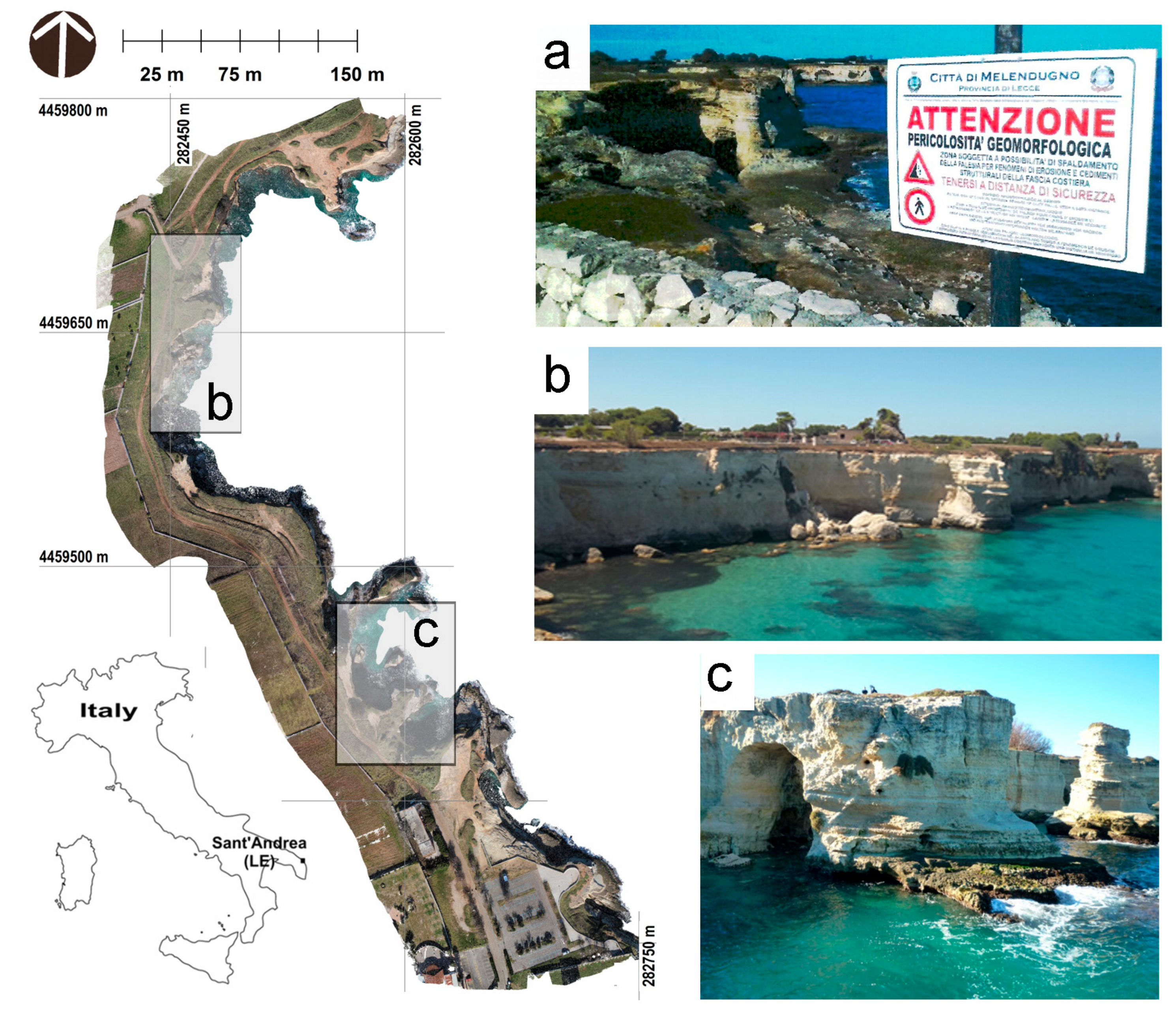
2. Study Area and Main Geological Setting

The methodology proposed in this study has been applied as a representative case study to a 600 m long portion of a coastal cliff located in Sant’Andrea, Melendugno (Apulia, Southern Italy). The cliff is characterized by a highly irregular geometrical setting, with a suggestive alternation of up to 10 m high vertical walls affected by frequent caves, arches and rock-stacks, and a sub-horizontal platform at the top. Since several years this portion of the cliff is subjected to erosive processes and instability phenomena, mainly represented by rock falls and block toppling. Consequently, a high-level geomorphological hazard has been assigned to the study area by the local authorities to prevent the involvement in the potential occurrence of rockfalls of people walking along the top of the cliff or boats approaching the cliff by the sea. Figure 1 reports the location of the study area and an orthophoto of the cliff portion examined which shows the effects of the different erosion rates affecting several portions of the cliff and the evidence of rock collapses. In particular, Figure 1b,c shows examples of the main geomorphological features resulting from such erosional and instability processes active along the cliff.
From a geological point of view, this area is characterized by the outcropping of a homogeneous calcarenite formation of Pliocene age, the Uggiano Formation [31] (see photos in Figure 1). In particular, throughout the study area, the sea cliffs are entirely formed of an alternation of coarse calcarenite layers, generally more resistant respect to the erosion processes, and finer calcilutite layers that are much more erodible than the calcarenite levels. This gives rise to a high selective erosion, with volumes of stiffer rock overhanging above the more erodible strata. In general, the erosion promoted by the sea water and the wave action is highly active along the lower strata of the cliff, while being of lower intensity in the upper portion. The rock is also affected by a limited number of joints resulting from tectonic and geological processes. However, most of the visible joints are the effect of the on-going instability processes that give rise to the unloading and stress relaxation in the mass, thus opening non-persistent fractures in the very shallow portion of the cliff. Sub-horizontal bedding joints are also not present in the rock mass, where only slight changes of the calcarenite facies due to variations of the cementation degree of the calcarenite can be observed. The present paper includes geomechanical analysis on a limited extent that appears to be almost massive and intact.
Different instability processes are active along the sea cliff in the study area. In particular, several blocks of few-meter size are present at the toe of the cliff and result from the detachment and fall of rock blocks overhanging because of the sea erosion in the lower strata (see Figure 1). The most diffuse instability phenomena throughout the area are represented by rockfalls, due to the detachment of overhanging rock blocks from the rock surface, and block toppling produced by the rotation of rock blocks eroded underneath that fall at the toe of the cliff [32]. These instability processes result from the brittle propagation of joints within the rock mass, starting from the areas where high shear and tensile stresses concentrate due to the local geometry of the cliff. It must be noted that the joints here referred are formed by the fragmentation and fracture propagation due to the loss of support of the rock blocks as an effect of erosion processes and due to the concentration of shear and tensile stresses. There is no in-situ evidence of relevant pre-existing joints in the rock mass able to affect the cliff stability.
Laboratory tests on calcarenite samples taken from the study area allowed to define the main physical and mechanical properties of the same rock. In particular, the rock unit weight and the uniaxial compression strength have been measured for both saturated and dry samples in order to derive the effects of rock saturation on the corresponding properties. Rock unit weight ranges between 15 and 17 kN/m3, whereas uniaxial compressive strength under saturated conditions results to be between 5 and 15 MPa, and the corresponding values under dry conditions are in the range between 12 and 25 MPa [33]. Based on these mechanical properties, the calcarenite examined can be classified as soft to moderately soft according to the classification proposed by Andriani and Walsh [33] and weak according to the ISRM one [34]. Referring to the minimum values of the compressive strength, a Mohr–Coulomb shear failure envelope has been defined, which is characterized by a cohesion c′ = 200–300 kPa and friction angle in the range between φ′ = 26°–34°.
Moreover, both short-term and long-term strength degradation processes are supposed to be highly active along the cliff, generally due to the environmental weathering [35]. However, with reference to coastal rock cliff, a faster and more intense weathering process of these calcarenite rocks results from the cyclic alternation of wetting and drying processes due to rainfall infiltration as well as from the marine salt crystallization following the contact with salt water. This is due to both the direct impact of the sea waves and the sea spray phenomena associated with the sea storms hitting the coast portion [36]. The sea water weathering is generally considered intense and aggressive on these calcarenite rocks, due to an effect of salt crystallization and bonding breakage, which results in a cementation reduction and a strength reduction of the rock in a relatively short-time period [36]. Therefore, instability processes triggered by weathering-induced rock degradation are relatively faster with respect to other areas characterized by calcarenite outcrops not affected by salt weathering [35,37].

3. Methodology: The Combination of UAV Photogrammetry and Three-Dimensional Finite Elements
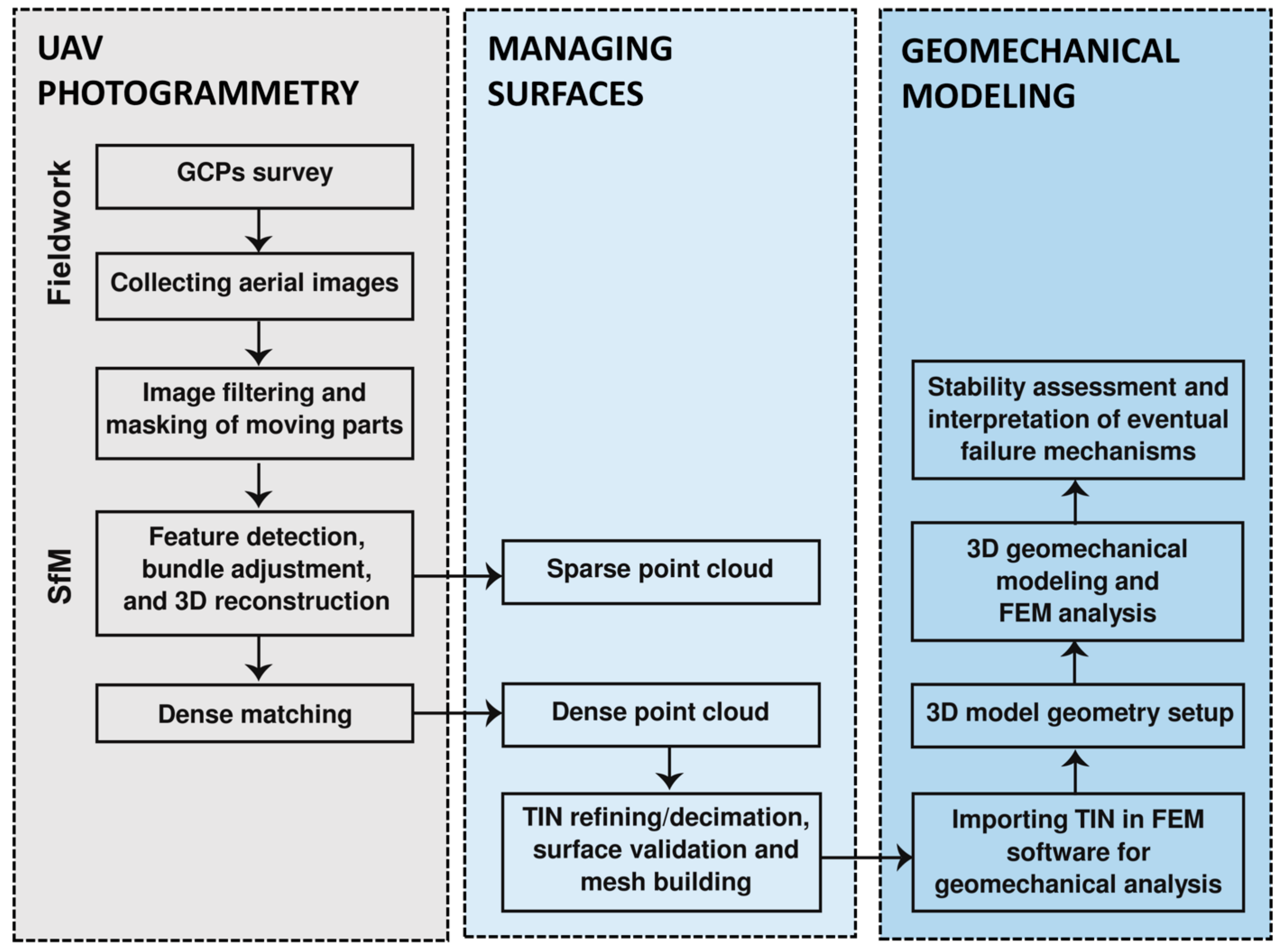
3.1. The Workflow

The methodology of integration between UAV photogrammetry to derive high resolution surface model of the rocky cliffs and successive application of geomechanical finite element modeling is summarized in Figure 2. In addition, the flowchart introduces the general organization of results reported in the present paper. To assess possible effect of mesh refining/decimation on the geomechanical modeling, several levels of surface simplification will be considered.

3.2. UAV Photogrammetry: Image Collection and Processing Strategy

The UAV airframe used was a hexacopter ESAFLY A2500 (designed and manufactured by SAL Engineering, Italy). The payload consisted of a Canon EOS 550D digital camera with focal length fixed at 25.0 mm during flights (sensor resolution: 5184 × 3456; average spatial resolution: at least 0.01 m) and navigation-grade GNSS receiver. By this configuration, the overall weight was 5.8 kg, which guaranteed a flight endurance of about 20 min. The aerial survey was carried out by nadir and oblique cameras. Three flights with a conventional parallel flight lines development were performed to cover the investigated area by nadir capture. These flights were planned using an aerial orthophoto as the reference map at an altitude of 50 m above ground level (a.g.l.) An autonomous mode of images acquisition with a shot per second was set. It resulted in 541 images acquired by the nadir camera with a forward and side overlap of 90% guaranteed. To collect aerial images of the sub-vertical portions of the sea cliff and represent complex topographic features with vertical development, additional oblique images were acquired by a single flight with a 60° off-nadir camera and manual piloting (flight line parallel to the seaside cliff profile). In total, 530 oblique aerial images were captured by the same equipment and timing at an average distance of 20 m from the cliff’s wall, thus producing a finer average spatial resolution. Blurred images and images acquired during the takeoff and landing operations were filtered out during the preliminary processing steps. The processing strategy consisted in the well-known SfM workflow to obtain a 3D georeferenced point cloud by reconstructing the camera pose and scene geometry simultaneously, through automatic identification of matching features in multiple images [38]. The scale-invariant feature-transform algorithm [39] detects and tracks these features from image to image, enabling the initial estimates of internal parameters, camera positions and object coordinates. Such parameters are then refined iteratively using nonlinear least squares minimization during the bundle adjustment step. Successively, the dense matching algorithms used the initial parameters to create the dense point cloud [40,41]. In the present study, the data were processed using the Agisoft PhotoScan photogrammetric software package (v.1.1.6, build 2038) and a standard approach to the images processing which include the usual steps: data import, image alignment, creation of the sparse cloud, optimization of image alignment and dense image matching. The dense cloud represents the reference surface for further three-dimensional geomechanical analysis based on finite element models.

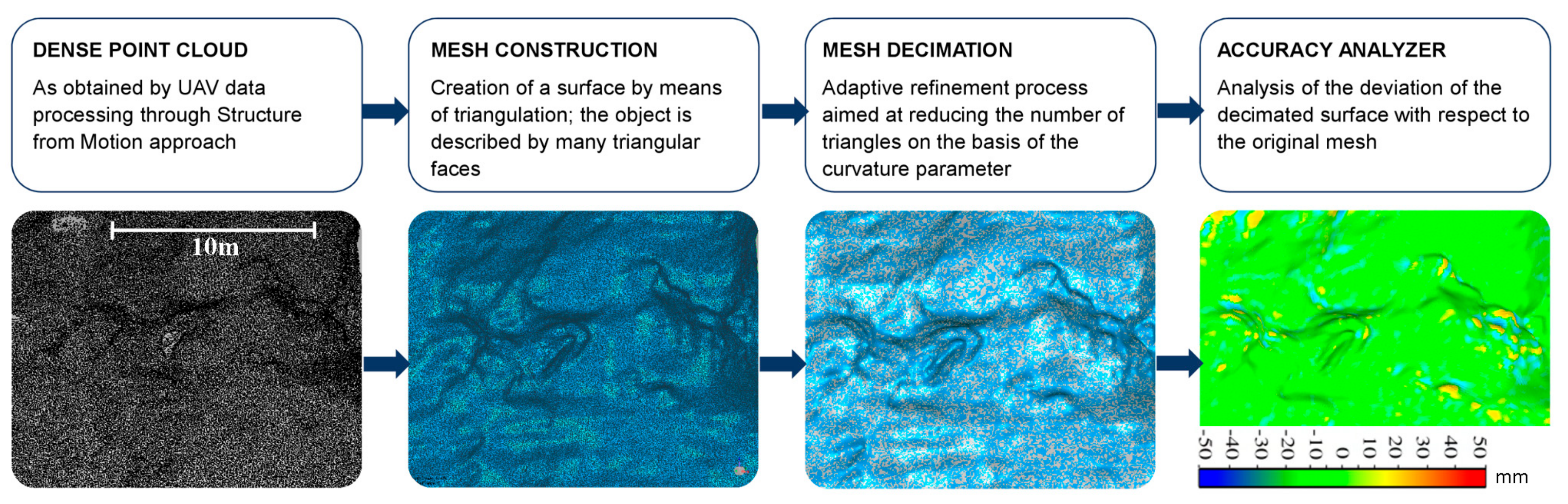
3.3. Managing Surfaces: Meshing Strategy of Point Cloud

As required by the geomechanical modeling suite, the dense point cloud obtained by UAV data processing was used to create a surface. Balancing the lower data storage requirements, while maintaining accuracy and efficiency in graphic manipulation, has always been a challenge for 3D geological and geomechanical modeling. Conventionally, surface models are being created using either regular grid or triangulated irregular network (TIN) techniques. Depending on the interpolation procedure, the accuracy of data represented through a regular grid model is relatively low, while TIN models are closer to the original point cloud. Despite a higher request in terms of data storage capacity, the TIN approach is the most widely adopted for accurately creating a surface starting from a point cloud. The majority of commercial software packages implement a triangulation approach, which is based on the 2.5-dimensions Delaunay algorithm [42]. This algorithm is widely used with terrain and environmental data while it encounters difficulties when manipulates steep or sub-vertical surfaces with complex geomorphic features. Such an approach could fail in the presence of narrowing patterns and inward shapes, which does not allow the projection onto a single virtual plane. The alternative approaches for triangulation proposed by Schumaker [43] provides a polygonal or polyhedral approximation of the desired object by generating poly-faces, the triangles, which follow the geometric shape of the point cloud. In the present work, the sea cliff surface will be initially reconstructed by means of triangular poly-faces with as much as possible uniform poly-edge lengths. By using the totality of vertices included in the dense point cloud the best surface resolution is achieved. The higher number of faces, thus requiring high storage capacity, will characterize the resulting meshed surface.
The search for a reliable and convenient surface for geomechanical modeling represents a key-factor. In particular, because of the large size of such models and limitation imposed by the geomechanical modeling suites, the import of data and successive processing could be challenging. Therefore, an optimization/refinement is required to reduce the dense cloud into a reliable three-dimensional model while preserving the full descriptive capacity and the ability to reconstruct the principal geological structures of the rock mass from the analysis of surface properties with further simplification of surface roughness. Moreover, the simplified model has to differentiate between geological structures (such as adjacent surfaces belonging to the same discontinuity set and adjacent surfaces belong to different sets). Nevertheless, the possible smoothing of sharp discontinuities delineated by the original model could compromise whatever structural analysis based on surfaces’ geometrical features. As refinement procedure, different strategies and degrees of decimation of polygons in the mesh could be implemented to optimize the dataset. Many of these utilize a penalty function that measures the errors in the surface properties incurred after a decimation process [44,45]. It could be accomplished using the original surface as benchmark in a distance analysis. Figure 3 summarizes the workflow followed in the present paper to provide a reliable surface obtained from UAV photogrammetry for further analysis and its validation.
In the attempt to preserve the ability to delineate the main geological structures from the surface analysis, in the present paper a criterion was selected. In particular, the decimation algorithm is forced to take into consideration the local surface curvature: the higher the curvature the lower the reduction ratio. In comparison with standard approaches to decimation, that homogeneously reduces the number of points depending on the chosen percentage of remaining points, the selected method was considered as more appropriate for natural irregular shapes. It is able to reduce the point density in flat surfaces while leaving the points distribution unchanged where discontinuities are found. Thus, the full descriptive capacity of the original dense point cloud is guaranteed. In these regions, the mesh representing the surface is fine while in regions where the surface is largely planar the density of the mesh can be coarser (in the present work this step has been carried out in Geomagic Studio v. 2013 suite with the Mesh tool Decimate). An example of different outcomes provided by standard and curvature-based approaches to the point cloud simplification is shown in Figure 4 for a small portion of the cliff surface (this area is also depicted in Figure 1b). In Figure 4, the decimation was at 4% of the full resolution, which represent one of the simplification levels used in the present paper.
As visible in Figure 4, the curvature-based approach shows higher point density in correspondence of surface discontinuities with respect to standard approach. By applying a 4% reduction rate to the original surface, the curvature-based approach shows a stronger reduction in point density of flat regions while points are preserved in correspondence of discontinuities.
The effects introduced by more or less conservative simplification procedure onto the quality of final models have to be monitored. Once the simplification criterion based on locale curvature analysis was selected, the level of similarity between surfaces could be also based on the assessment of deviation between the decimated surface and the original undecimated mesh in terms of absolute distances between surfaces along a preferred direction or eventual changing in the main geometrical features. Thus, in the attempt to proceed with simplification of original surfaces without altering the geometrical properties of the virtual sea cliff, a threshold of 5 cm has been selected as limit in the deviation between decimated and undecimated (full resolution) surfaces. Such value of accuracy is comparable with the average roughness of the planes and is fully compatible with the 1:1000 precision rates introduced by James and Robson [17] (in the present paper, the ratios refer to the maximum flight altitude of 50 m a.g.l. during flight with nadir cameras). Considering the shorter distances between cameras and the rocky cliff adopted during flight with oblique cameras, such threshold could be considered as precautionary. However, the geomechanical modeling could be very sensitive to changes in the morphometry of the cliff surfaces due to successive simplification procedures.

3.4. Three-Dimensional Finite Element Models for Geomechanical Analyses

A detailed quantitative assessment of the stability conditions of a rock cliff requires the application of numerical modeling to the problem examined to explore the evolution of the stress-strain state of the rock mass during the specific stage of the cliff history examined. Numerical methods, which can implement the field equations that govern the whole problem, represent the most advanced tool available to explore the potential rock cliff instability mechanisms, which could be only based on investigations and surveys carried out through phenomenological studies. In the last years, several papers faced the application of numerical methods to the analysis of the triggering mechanisms and/or the evolution of rock mass instability processes. Some of them highlighted the potentialities of methods such as finite element, discrete element or hybrid finite-discrete element methods [37,46,47,48]. Generally, the correct simulation of the behavior of a rock mass in a finite element model requires the assessment of several factors regarding the rock mass geometry, the rock constitutive model to be adopted and the corresponding geomechanical properties of the rock mass, the mechanical boundary conditions of the model, the initial stress state of the rock mass, and, finally, the simulation of the physical processes that are supposed to control the triggering of the instability process. For those problems where rock weathering is supposed to be dominant, the simulation of the weathering conditions affecting the examined rock masses can have a large impact on the accuracy of the modeling results. Based on the specific problem analyzed, the variation of the rock mass properties due to the environmental weathering processes should be adequately implemented by means of simplified uncoupled or more sophisticated chemo-mechanical analyses [35,37,49]. In the present paper, the three-dimensional finite element model of the rock cliff examined has been developed by means of PLAXIS-3D (PLAXIS-BV 2013, Delft, The Netherlands) to simulate the current stress–strain state of the rock mass and its potential evolution with time.

4. Results

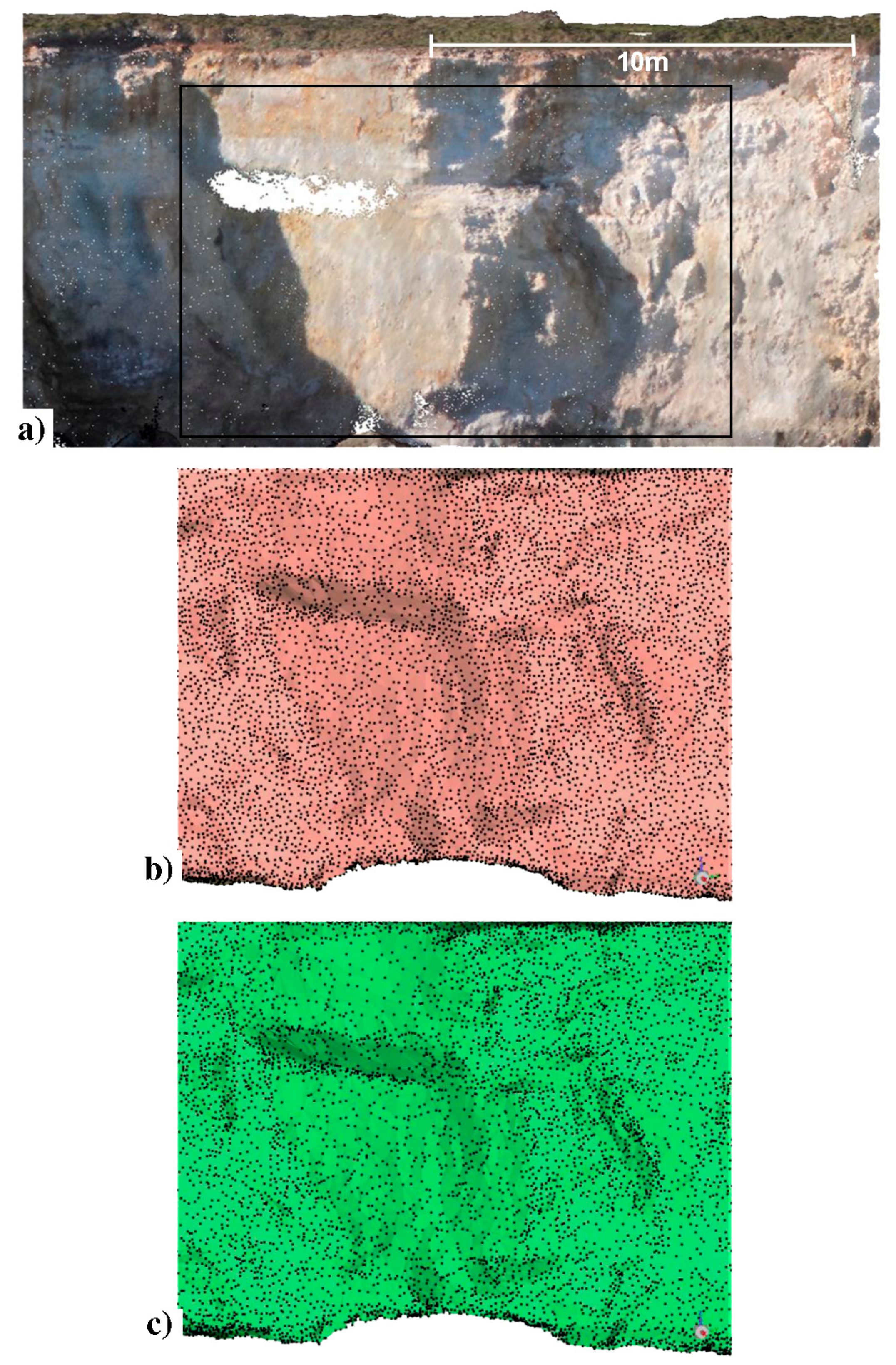
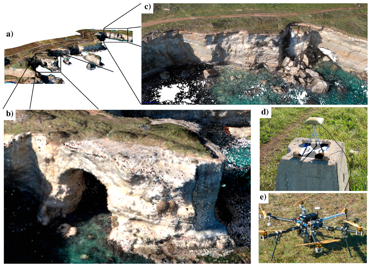
4.1. Point-Cloud Generation from UAV Images

The external orientation of point cloud was achieved by the survey of 13 evenly spaced ground control points (GCP) through survey-grade GNSS receivers (Topocon GB100 dual frequency model) and a static relative GNSS positioning, providing a final positional accuracy of GCPs at cm-level. To achieve such an accuracy, a reference station was set in the study area and its coordinates derived thanks to the computation and adjustment of two baselines connecting the reference station with two permanent GNSS stations belonging to the Apulian GNSS positioning facility (Regione Puglia GNSS Network, Reference Station Service Provider). Such stations are located at Giurdignano (Lecce) and Salice Salentino (Lecce) at an average distance of 40 km from the GNSS station set in the study area. Raw data acquired during the four hours long static surveys were post-processed with the Leica Geomatic Office package. GCPs were mainly located atop the cliff, at a mutual average distance of 50 m, with just one located over an accessible natural terrace located in the lower part and none located on the vertical surfaces of the cliff due to logistic constraints and unsafe conditions for personnel.
The 541 nadir and off-nadir images were processed simultaneously during the SfM workflow and the GCPs used in the bundle adjustment as constraint to create the model in a specific reference system (GCPs’ accuracy equal to 0.010 m). It resulted in a dense cloud composed of 13,255,337 points. Figure 5 depicts the dense point clouds of the investigated area (Figure 5a), and local geological features (Figure 5b,c) in addition to one of the targets used (Figure 5d) and the hexacopter (Figure 5e).
Being very difficult any survey with other technology, a reference model of the sea cliff was not available and the absolute accuracy of 3D-reconstruction process of the coastal cliff could not be validated. However, the geomechanical model is more sensitive to a close reconstruction of surface features and their orientations rather than the accuracy in the absolute positioning of the point cloud. In a previous paper, the present authors verified the ability to accurately map natural landforms with sub-vertical development by the combination of nadir and oblique images by adopting the same equipment and survey strategy [50].

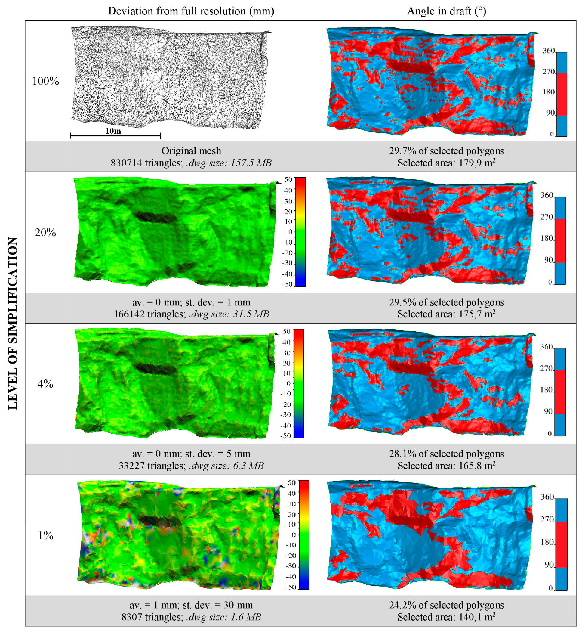
4.2. Building and Validating TIN Surfaces at Changing Resolution

Due to the mentioned computational limitation in the use of very dense point cloud, in this paper, we adopted several levels of decimation of the original TIN surfaces (100% of the available point cloud) towards decimated versions (20%, 4%, and 1% of the original surfaces). The average density of the point cloud was 730 pts/m2 at full resolution. The density decreased to 155 pts/m2, 21 pts/m2 and 8 pts/m2 at 20%, 4% and 1% level of simplification, respectively. These levels of simplification were arbitrarily selected to achieve a significant reduction in point density and a reduction factor of five between successive simplifications (the 1% level was selected in place of 0.8%). An inspection of some morphometric features could provide a contribution to the procedure of surface validation. Figure 6 shows the effect of successive cloud decimations by a couple of them; the distance between original and decimated surfaces along the local normal direction and the values of the angle in draft. By defining positive values of the vertical in the up direction and a draft angle = 0° polygons with negative normal values along the z axis can be selected. Results achieved by such analyses have been mapped over a limited portion of the cliff (the whole extent shown in Figure 4a and also depicted in Figure 1b).
The deviation analysis in Figure 6 shows a significant decrease in the number of triangles and vector files size when the level of simplification increases from 100 to 1%. Certainly, it facilitates the FEM analysis but the geometric accuracy of the surface has to be assessed further. The distance between the decimated and original surfaces shows average values close to zero mm in most cases and rarely reaches values of 50 mm, thus, without affecting in a significant manner the surfaces representation. By paying attention to the surface curvature while reducing the original surface at 1% of the full resolution, the simplified dataset does not differ in a significant manner. The angle in draft analysis can highlight sectors of the sea cliff with specific settings. In particular, the selected angle in draft put the overhanging sectors of the rocky cliff into evidence on the surfaces at 100%, 20%, 4%, and 1% level of simplification (see red areas representing orientation of surfaces from 90° to 270° with respect to the up direction). By reducing the surface complexity, such characteristic seems to be almost completely preserved, with only a reduction of selected features for very small surface features. Due to these findings, the simplified surface at 1% and 4% of the full resolution can be considered as suitable for geomechanical modeling and the decimation based on surface curvature very effective for proposed investigation.

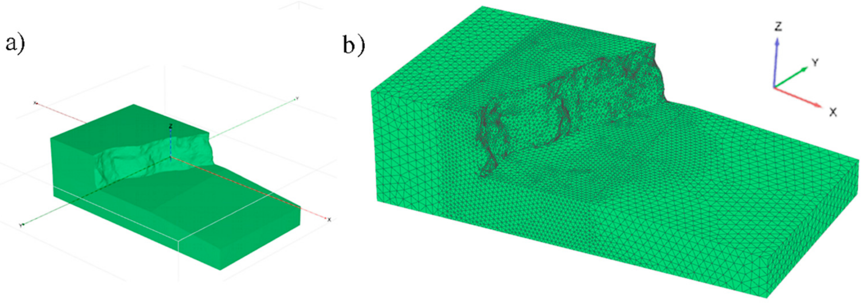
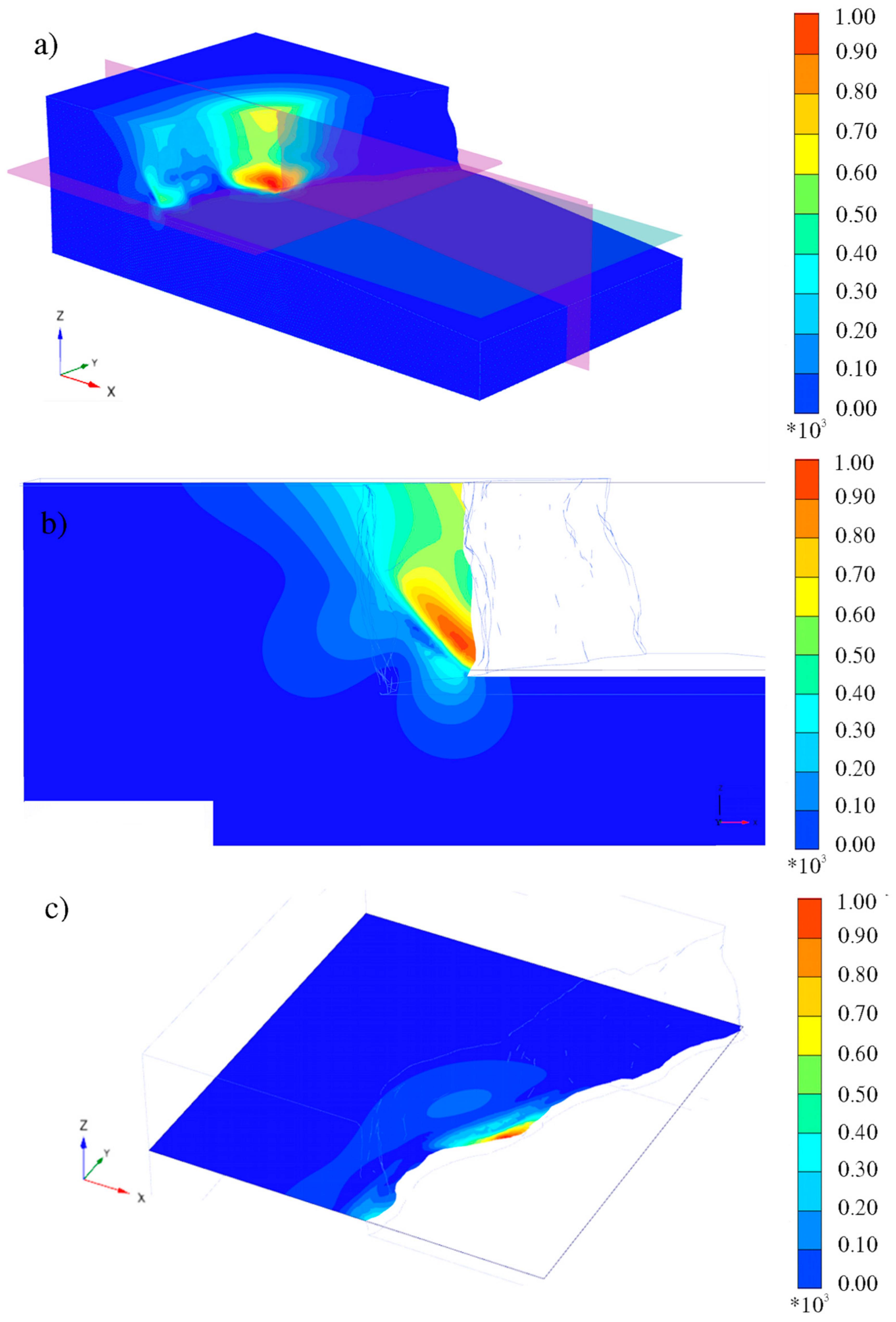
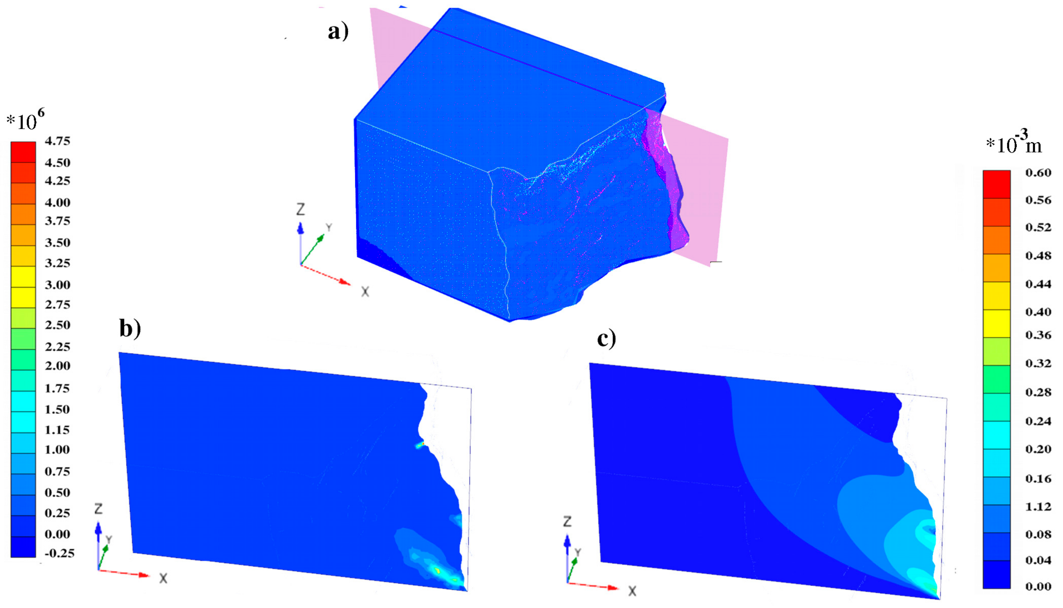
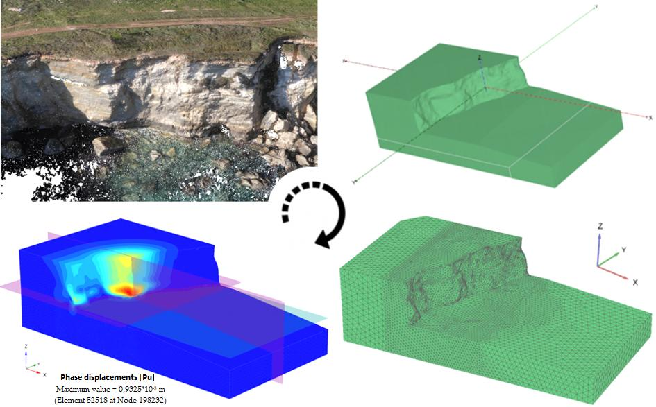
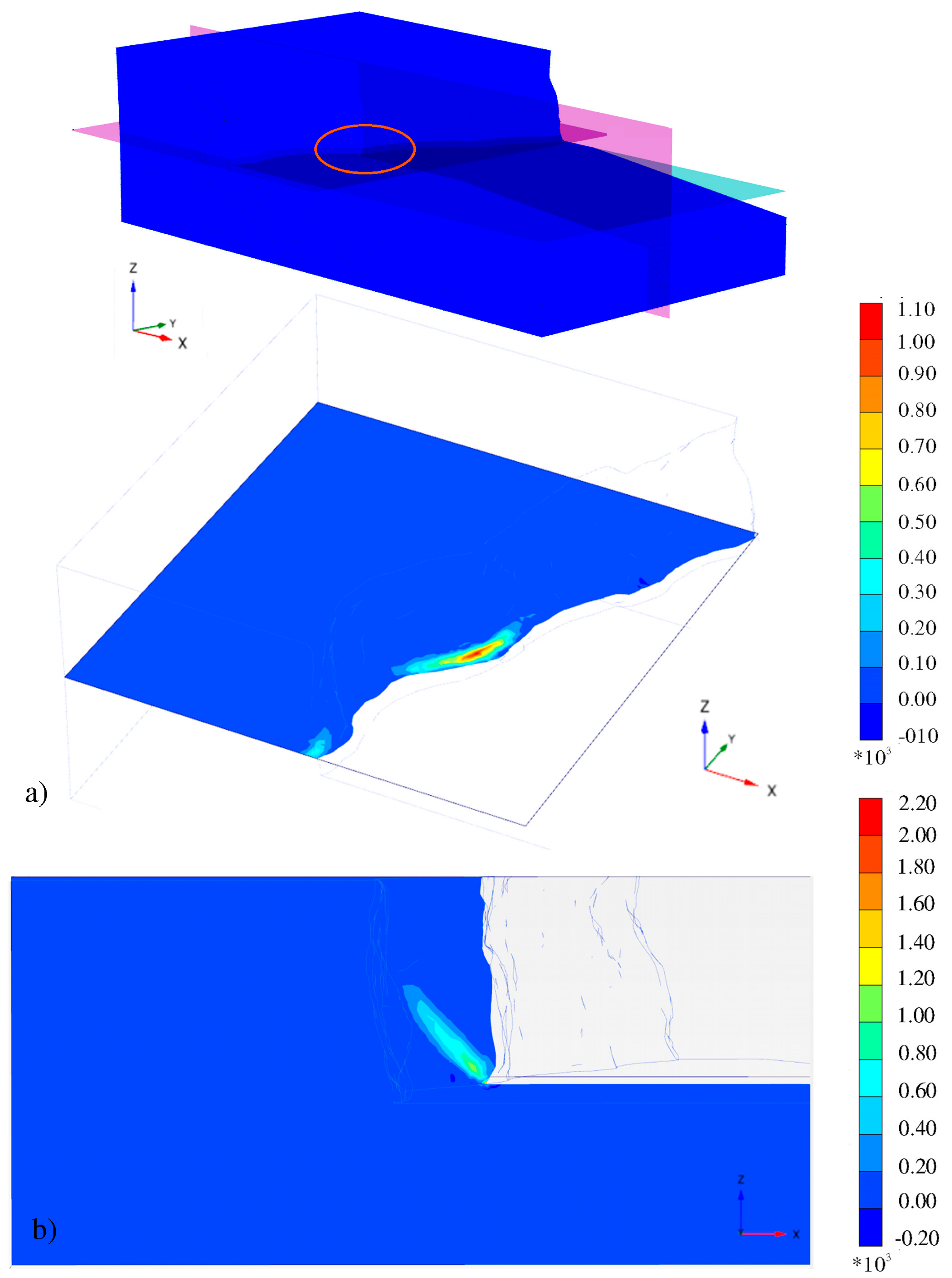
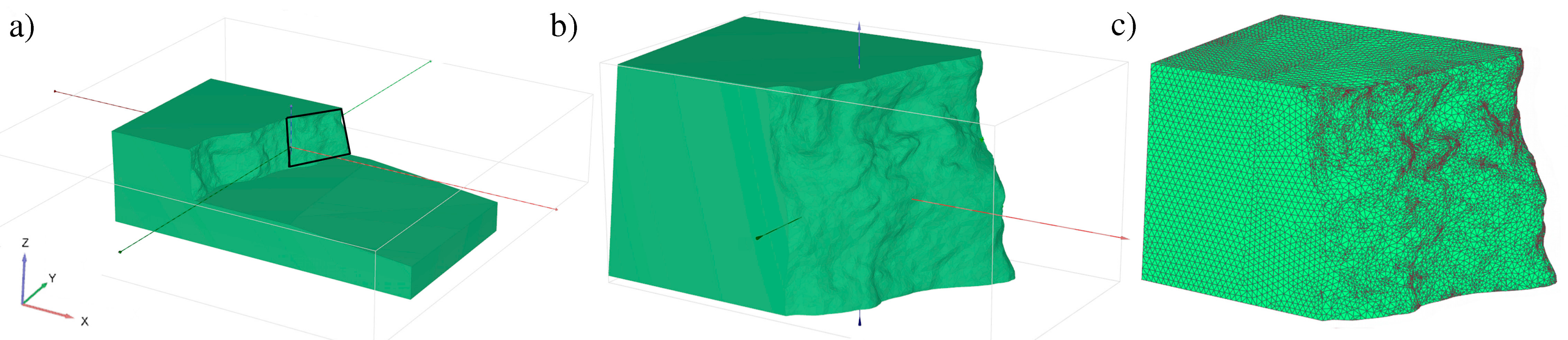
4.3. Finite Element Model of the Rock Cliff: Surface Importing, Model Construction and Main Results

The solid forming the whole analysis domain is shown in Figure 7 and derives from importing in the FEM code the 3D TIN surface of the rock cliff sector depicted in Figure 4a at 1% of the full resolution. Then, the domain has been built by extruding the surface in the x-direction and adding an approximate geometry of the rock volume below the sea surface characterized by a very low slope gradient. A vertical side boundary has been imposed to delimit the numerical domain in the x-direction, at a minimum distance of 20 m from the cliff surface in order to reduce the risk of end effects in the computational results, as well as two vertical boundaries have been assigned to delimit the domain in the y-direction. The numerical model has been also delimited by a horizontal surface at the top of the cliff, where ground surface is practically flat, and at the bottom of the domain. The three-dimensional discretization mesh is composed of 273,074 tetrahedral elements and is the result of a compromise between accuracy of the calculation and computational costs, whereas the number of nodes forming the 3D domain is equal to 386,974. The volume close to the cliff surface has been discretized with a very fine mesh (average element size = 0.48 m), whereas the remaining portion of the model has been discretized with a significantly coarser mesh (average size = 2.7 m).
An elastic–perfectly plastic constitutive model, with a Mohr–Coulomb failure criterion, non-associated flow (ψ = 0°) and tension cut-off, has been adopted for the calcarenite rock material to explore the areas where the onset of rock failure is reached, along with the corresponding failure mechanism. The parameter values adopted to characterize the calcarenite according to the Mohr-Coulomb model are reported in Table 1.
These parameters are representative of saturated conditions of the calcarenite, which correspond to the lower rock strength parameters and, therefore, to the most adverse conditions for rock stability. The analyses have been carried out under drained conditions and assuming the portion of the domain above the sea surface as above the water table.
Three stages of analysis have been assigned in the model: Phase 1 is represented by the assignment of the initial stress state. In Phase 2, the elasto-plastic behavior for the rock material has been assigned in accordance with the adopted parameters. Then, after numerical convergence is reached in the second stage analysis, which means stable conditions resulting from the model, a third stage, represented by a “strength reduction” analysis [51], has been performed in order to evaluate the safety factor SF along with the mobilized rock strength at failure (Phase 3).
The value of the rock cohesion has been set as variable to derive the conditions that give rise to the collapse of the cliff, whereas the friction angle value has been kept fixed. This reflects the process of reduction of the cementation as induced by environmental weathering in carbonate rocks [35,36,52], which can develop both in the short-term, that is after calcarenite saturation, and in the long-term, due to cyclic drying-wetting processes as well as after contact with salt water. In the proposed modeling, no different weathering rates has been assumed along the cliff surface and a uniform weathering degree for the whole cliff has been accounted for.
Starting from the initial value of c′ = 150 kPa, which represents a typical value of cohesion for the calcarenite examined under saturated conditions, cohesion c′ has been gradually reduced to assess the values corresponding to the occurrence of a cliff instability process. Assuming a value of c′ = 40 kPa the numerical results indicate a safety factor approximately equal to SF = 1.3. When the cohesion value is furtherly reduced, the safety factor progressively decreases. The cliff experiences failure when a cohesion value ranging between 30 and 35 kPa is assumed. Figure 8a,b show respectively a two-dimensional horizontal and vertical cross section of the contours of the cumulated deviatoric strains. It indicates that a strain mechanism develops in the central protruding volume of the cliff, starting from the toe of the cliff according to a high inclination, and then propagating about parallel to the cliff surface up to the top of the cliff structure.
The displacement field associated to this strain mechanism is shown in Figure 9a, where the three-dimensional contours of the vertical displacements are reported, whereas Figure 9b,c depicts the same contours in the vertical and horizontal cross-sections indicated in Figure 9a. Figure 9 confirms that the potentially unstable rock volume is limited to the protruding cliff portion, characterized by no lateral confinement. As shown in Figure 9a, the rock volume that tends to become unstable is of the same order of magnitude of the rock column already collapsed shown in Figure 5c, which is located at the right side of the cliff portion examined in the model here presented.
To explore the effect introduced by the surface decimation in the numerical modeling, the FE analysis was also performed from the 3D TIN surface of the rock cliff with a 4% level of simplification with respect to the original surface. In particular, the analysis was limited to the right-hand side of the whole cliff portion modeled in the 1% decimation analysis (see Figure 10). Then, the domain has been built by extruding the surface in the x-direction. To focus specifically on the potential instability of local areas of the cliff, in this model, only the cliff portion above the sea level has been accounted for. A vertical side boundary has been imposed to delimit the numerical domain in the x-direction as well as two vertical boundaries have been assigned to delimit the domain in the y-direction. The numerical model has been also delimited by a horizontal surface at the top of the cliff and at the bottom of the domain, at the sea level (see Figure 10a). The three-dimensional discretization mesh is composed of 302,865 tetrahedral elements and 429,195 nodes; the mesh is very fine (average element size = 0.1 m) along the cliff surface and is coarser (average size = 1 m) in the inner portion of the solid (Figure 10b,c).
The same numerical assumptions of the previous model have been adopted in this specific model. In this case, when the cohesion value is reduced to values ranging between 20 and 30 kPa, the cliff results to be unstable. By considering the cross section depicted in Figure 11a,b shows a two-dimensional cross section of the contours of the incremental deviatoric strains, whereas Figure 11c reports the corresponding contours of cumulated displacements. The images in Figure 11b,c suggest a strain mechanisms that propagates from the toe of the cliff up to the mid of the cliff, delimiting the protruding portion of the cliff in the same area.
The 4% decimation analysis shows the tendency of the propagation of deviatoric strains and cumulated displacements from the toe to the mid area of the cliff, although these are not evident as in the larger model (Figure 7, Figure 8 and Figure 9), which instead reveals larger strain levels and highlights the failure mechanism in the central area. However, the comparison between the two models shows the finer spatial modeling of the analysis based on the surface at 4% simplification level, which can be used as a detailed model focusing on the stability of specific cliff portions, i.e., local failure mechanisms. Global failure mechanism detected in the central area could not be simulated correctly with the model at 4% level of simplification. On the contrary, such mechanism has been characterized by the analysis performed from the surface based on the higher level of decimation (1% of the full resolution).

5. Discussion

The methodology described in the previous sections shows that the combination of UAV photogrammetry and geomechanical modeling is able to cover a gap in the investigation of the stability of long sectors of coastal rocky cliffs, so that an accurate three-dimensional finite element model has been developed based on a detailed geometrical survey of the rock surface. To this purpose, both a methodological procedure to manage the point clouds resulting from the UAV survey and a procedure to decimate the point clouds aimed at allowing for importing into commercial 3-D FEM geomechanical models have been proposed. In particular, a FEM model developed by importing a 1% point cloud decimation surface has been carried out for a limited part of the extensive morphological data detected with UAV, whereas a 4% decimation model has been performed with respect to a smaller portion of the same surface. The decimation procedures and the consequent reduction of the modeling areas arise from the need to make the point clouds compatible with the computational capacity of commercial geomechanical calculation codes running on ordinary-capacity workstations.
The analysis based on cliff surface after the decimation at 4% of the full resolution (see Figure 10 and Figure 11) results to be unstable when a cohesion value lower than 30 kPa is adopted for the rock material. By using these values, a lack of numerical convergence is observed and a clear tendency of the deviatoric strains to delimit a slice of rock prone to instability comes out from the model results. Instead, the analysis performed after the decimation at 1% provides indication of the occurrence of a general failure mechanism characterized by the development of shear failures starting from the toe with a high inclination and then propagating about parallel to the cliff surface, up to the top of the cliff. This phenomenon is visible in Figure 8 and Figure 9, when a cohesion value of 35 kPa is adopted.
It comes out that the 1% decimation model, involving a significantly larger cliff surface, resulted to be more unstable with respect to the 4% decimation model, the latter requiring a lower value of cohesion to trigger instability. These results are supposed to be an effect of the three-dimensional geometry of the cliff in the two models examined, since the larger 1% decimation model is characterized by a central area with protruding geometry (i.e., with no lateral confinement) where instability seems to be more likely. This suggests that these numerical models can be effectively applied to explore the effects of three-dimensionality, in terms of both general, i.e., failure mechanisms involving the whole cliff height, and local stability, i.e., the eventual occurrence of smaller rockfalls. Therefore, less accurate models (1% decimation) can be used to analyze large cliff portions to explore the general stability of the cliff and detect the areas potentially critical, whereas more accurate models focusing on specific areas can be used to investigate the potential occurrence of local instability mechanisms.
In comparison with geomechanical analysis based on 2D modeling, the three-dimensional approach for structures with sub-vertical setting, as is the case study proposed in the present paper, allows for a more reliable simulation about in-situ stress–strain states existing in the rock mass and the effects produced by the presence of lateral confinement. In particular, 3D models allowed for simulating the existence of protruding rock volumes (i.e., with no lateral confinement) or, alternatively, rock volumes highly confined in the direction parallel to the cliff. On the contrary, geomechanical analysis based on 2D models remains a fundamental approach in the investigation of the plane–strain behavior using a reference plane along a normal direction to the cliff. This is also the case of the present study, where instability conditions for a protruding volume of the cliff due to the absence of lateral confinement have been detected by the proposed 3D geomechanical modeling [53,54].

6. Conclusions

Results provided by the present paper show that the combination of UAV photogrammetry and geomechanical modeling is able to cover a gap in the investigation of the stability of long sectors of coastal rocky cliffs when no information could be acquired by alternative surveying methodologies due to the absence of vantage points to make stationing. The fieldwork is limited to the surveying of few accurate control points and the whole procedure could represent a rapid and highly automated investigation of hazards to slope failure in coastal areas. Indeed, the importing of dense surface models and the accuracy of corresponding geomechanical numerical analyses still represent open issues due to the extremely high density of points generated from the photogrammetric processing of UAV images. Thus, a refinement/decimation procedure is required by the geomechanical finite element modeling to have a feasible analysis at varying spatial scale. We found that, in the present study, decimation algorithms based on the preservation of more complex surface features can reduce the model size at 1% or 4% of the original size without significant loss of descriptive capacity. The geomechanical finite element modeling performed on a test area by importing the reduced-size surface is relatively insensitive to such degrees of simplification, since both the 1% and the 4% size models provided about the same results in terms of mobilized strength of the rock material. In particular, the numerical results indicate failure mechanisms due to possible propagation of shear fractures that involve protruding cliff volumes.
It is worthwhile pointing out that, in the geomechanical model here proposed, rock discontinuities have not been accounted for, since, in the specific case study, they are of limited number and do not have geological or tectonical origin. Since they generally represent the effect of on-going failure processes the assumption of a continuous rock mass is acceptable here. However, in general, the presence of structural joints within the rock mass examined is highly frequent and in the corresponding numerical model can be accounted for by introducing interface elements. This perspective is supposed to be explored in a future work.
Despite the feasibility of the proposed methodology, future works have to deal with the increasing necessity to process three-dimensional dataset at finer resolution and collected over large extents. Alternative approaches could be based on a different strategy for data organization without loss of accuracy and more convenient files for further modeling. An effective solution to model natural environments could be the design of NURBS (Non-Uniform Rational B-Spline) surface patch, a representation that is already and extensively used in the free form representation of objects because of its ability to model complex free-form curves and surfaces [55,56].

Acknowledgments

Field test carried out within the PRIN 2010–2011 were financed by the Italian Ministry of Education, University and Research.

Author Contributions

F.M. conceived and designed the experiments, wrote the introductory parts, sections related to the UAV survey and data processing, and wrote final comments; M.D. performed the UAV flight and terrestrial survey on-site for GCP location; C.C. defined the meshing strategy, faced the validation of surface data and wrote the relevant section; P.R. processed the UAV images to derive the three-dimensional model; N.L.F designed the use of geomechanical model with UAV data and managed the relevant data processing; M.P. provided the main contribution in the geomechanical modeling; and P.L. investigated the geological setting of the area and wrote the sections relevant to the geomechanical modeling and discussions.

Conflicts of Interest

The authors declare no conflict of interest.

References

  1. Corsini, A.; Castagnetti, C.; Bertacchini, E.; Rivola, R.; Ronchetti, F.; Capra, A. Integrating airborne and multi-temporal long-range terrestrial laser scanning with total station measurements for mapping and monitoring a compound slow moving rock slide. Earth Surf. Proc. Landf. 2013, 38, 1330–1338. [Google Scholar] [CrossRef]
  2. Assali, P.; Grussenmeyer, P.; Villemin, T.; Pollet, N.; Viguier, F. Surveying and modeling of rock discontinuities by terrestrial laser scanning and photogrammetry: Semi-automatic approaches for linear outcrop inspection. J. Struct. Geol. 2014, 66, 102–114. [Google Scholar] [CrossRef]
  3. Bemis, S.P.; Micklethwaite, S.; Turner, D.; James, M.R.; Akciz, S.; Thiele, S.T.; Bangash, H.A. Ground-based and UAV-based photogrammetry: A multi-scale, high-resolution mapping tool for structural geology and paleoseismology. J. Struct. Geol. 2014, 69, 163–178. [Google Scholar] [CrossRef]
  4. Cawood, A.J.; Bond, C.E.; Howell, J.A.; Butler, R.W.; Totake, Y. LiDAR, UAV or compass-clinometer? Accuracy, coverage and the effects on structural models. J. Struct. Geol. 2017, 98, 67–82. [Google Scholar] [CrossRef]
  5. Michoud, C.; Carrea, D.; Costa, S.; Derron, M.H.; Jaboyedoff, M.; Delacourt, C.; Maquaire, O.; Letortu, P.; Davidson, R. Landslide detection and monitoring capability of boat-based mobile laser scanning along Dieppe coastal cliffs, Normandy. Landslides 2015, 12, 403–418. [Google Scholar] [CrossRef]
  6. Rosnell, T.; Honkavaara, E. Point cloud generation from aerial image data acquired by a quadrocopter type micro unmanned aerial vehicle and a digital still camera. Sensors 2012, 12, 453–480. [Google Scholar] [CrossRef] [PubMed]
  7. Watts, A.C.; Ambrosia, V.G.; Hinkley, E.A. Unmanned aircraft systems in remote sensing and scientific research: Classification and considerations of use. Remote Sens. 2012, 4, 1671–1692. [Google Scholar] [CrossRef]
  8. Westoby, M.J.; Brasington, J.; Glasser, N.F.; Hambrey, M.J.; Reynolds, J.M. ‘Structure-from-Motion’photogrammetry: A low-cost, effective tool for geoscience applications. Geomorphology 2012, 179, 300–314. [Google Scholar] [CrossRef] [Green Version]
  9. Bryson, M.; Johnson-Roberson, M.; Murphy, R.J.; Bongiorno, D. Kite aerial photography for low-cost, ultra-high spatial resolution multi-spectral mapping of intertidal landscapes. PLoS ONE 2013, 8, e73550. [Google Scholar] [CrossRef] [PubMed]
  10. Mancini, F.; Dubbini, M.; Gattelli, M.; Stecchi, F.; Fabbri, S.; Gabbianelli, G. Using unmanned aerial vehicles (UAV) for high-resolution reconstruction of topography: The structure from motion approach on coastal environments. Remote Sens. 2013, 5, 6880–6898. [Google Scholar] [CrossRef] [Green Version]
  11. Fonstad, M.A.; Dietrich, J.T.; Courville, B.C.; Jensen, J.L.; Carbonneau, P.E. Topographic structure from motion: A new development in photogrammetric measurement. Earth Surf. Process. Landf. 2013, 38, 421–430. [Google Scholar] [CrossRef]
  12. Rupnik, E.; Nex, F.; Remondino, F. Oblique multi-camera systems-orientation and dense matching issues. In EuroCOW 2014, Proceedings of the European Calibration and Orientation Workshop, Castelldefels, Spain, 12–14 February 2014; The International Archives of Photogrammetry, Remote Sensing and Spatial Information Sciences: Kreuztal, Germany, 2014; Volume XL-3/W1, pp. 107–114. [Google Scholar] [CrossRef]
  13. Clapuyt, F.; Vanacker, V.; Van Oost, K. Reproducibility of UAV-based earth topography reconstructions based on Structure-from-Motion algorithms. Geomorphology 2016, 260, 4–15. [Google Scholar] [CrossRef]
  14. Harwin, S.; Lucieer, A.; Osborn, J. The impact of the calibration method on the accuracy of point clouds derived using unmanned aerial vehicle multi-view stereopsis. Remote Sens. 2015, 7, 11933–11953. [Google Scholar] [CrossRef]
  15. Agüera-Vega, F.; Carvajal-Ramírez, F.; Martínez-Carricondo, P. Accuracy of digital surface models and orthophotos derived from unmanned aerial vehicle photogrammetry. J. Surv. Eng. 2016, 143, 04016025. [Google Scholar] [CrossRef]
  16. Eltner, A.; Kaiser, A.; Castillo, C.; Rock, G.; Neugirg, F.; Abellán, A. Image-based surface reconstruction in geomorphometry–merits, limits and developments. Earth Surf. Dyn. 2016, 4, 359–389. [Google Scholar] [CrossRef]
  17. James, M.R.; Robson, S. Straightforward reconstruction of 3D surfaces and topography with a camera: Accuracy and geoscience application. J. Geophys. Res. Earth 2012, 117. [Google Scholar] [CrossRef] [Green Version]
  18. Genchi, S.A.; Vitale, A.J.; Perillo, G.M.; Delrieux, C.A. Structure-from-motion approach for characterization of bioerosion patterns using UAV imagery. Sensors 2015, 15, 3593–3609. [Google Scholar] [CrossRef] [PubMed]
  19. Warrick, J.A.; Ritchie, A.C.; Adelman, G.; Adelman, K.; Limber, P.W. New techniques to measure cliff change from historical oblique aerial photographs and Structure-from-Motion photogrammetry. J. Coast. Res. 2016, 33, 39–55. [Google Scholar] [CrossRef]
  20. Danzi, M.; Di Crescenzo, G.; Ramondini, M.; Santo, A. Use of unmanned aerial vehicles (UAVs) for photogrammetric surveys in rockfall instability studies. Rend. Online Soc. Geol. Ital. 2012, 24, 82–85. [Google Scholar]
  21. Nex, F.; Remondino, F. UAV for 3D mapping applications: a review. Appl. Geomat. 2014, 6, 1–15. [Google Scholar] [CrossRef]
  22. Giordan, D.; Manconi, A.; Facello, A.; Baldo, M.; Dell’Anese, F.; Allasia, P.; Dutto, F. Brief Communication: The use of an unmanned aerial vehicle in a rockfall emergency scenario. Nat. Hazards Earth Syst. Sci. 2015, 15, 163–169. [Google Scholar] [CrossRef]
  23. Dewez, T.J.B.; Leroux, J.; Morelli, S. Cliff collapse hazard from repeated multicopter UAV acquisitions: return on experience. In Proceedings of the XXIII ISPRS Congress, Prague, Czech Republic, 12–19 July 2016; Volume XLI-B5. [Google Scholar] [CrossRef]
  24. Piras, M.; Taddia, G.; Forno, M.G.; Gattiglio, M.; Aicardi, I.; Dabove, P.; Lo Russo, S.; Lingua, A. Detailed geological mapping in mountain areas using an unmanned aerial vehicle: application to the Rodoretto Valley, NW Italian Alps. Geomat. Nat. Hazards Risk 2017, 8, 137–149. [Google Scholar] [CrossRef]
  25. Quinn, J.D.; Rosser, N.J.; Murphy, W.; Lawrence, J.A. Identifying the behavioural characteristics of clay cliffs using intensive monitoring and geotechnical numerical modelling. Geomorphology 2010, 120, 107–122. [Google Scholar] [CrossRef]
  26. Ferrero, A.M.; Migliazza, M.; Roncella, R.; Rabbi, E. Rock slopes risk assessment based on advanced geostructural survey techniques. Landslides 2011, 8, 221–231. [Google Scholar] [CrossRef]
  27. Martino, S.; Mazzanti, P. Integrating geomechanical surveys and remote sensing for sea cliff slope stability analysis: the Mt. Pucci case study (Italy). Nat. Hazards Earth Syst. Sci. 2014, 14, 831–848. [Google Scholar] [CrossRef]
  28. Riquelme, A.J.; Tomás, R.; Abellán, A. Characterization of rock slopes through slope mass rating using 3D point clouds. Int. J. Rock Mech. Min. Sci. 2016, 84, 165–176. [Google Scholar] [CrossRef] [Green Version]
  29. Abellan, A.; Derron, M.H.; Jaboyedoff, M. Use of 3D Point Clouds in Geohazards. Remote Sens. 2016, 8, 130. [Google Scholar] [CrossRef]
  30. Balek, J.; Blahůt, J. A critical evaluation of the use of an inexpensive camera mounted on a recreational unmanned aerial vehicle as a tool for landslide research. Landslides 2017, 14, 1217–1224. [Google Scholar] [CrossRef]
  31. Largaiolli, T.; Martinis, B.; Mozzi, G.; Nardin, M.; Rossi, D.; Ungaro, S. Note illustrative della Carta Geologica d'Italia, Foglio 214, Gallipoli; Servizio Geologico d’Italia: Rome, Italy, 1969; 64p. (In Italian) [Google Scholar]
  32. Cruden, D.M.; Varnes, D.J. Landslide Types and Processes. In Landslides: Investigation and Mitigation; Turner, A.K., Schuster, R.L., Eds.; National Research Council: Washington, DC, USA, 1996; pp. 36–75, 247. [Google Scholar]
  33. Andriani, G.F.; Walsh, N. Petrophysical and mechanical properties of soft and porous building rocks used in Apulian monuments (south Italy). In Natural Stone Resources for Historical Monuments—Geological Society Special Publication (Book 333); Prikryl, R., Smith, B.J., Eds.; Geological Society of London: London, UK, 2010; pp. 129–141. [Google Scholar]
  34. International Society of Rock Mechanics. Suggested methods for the quantitative descriptions of discontinuities in rock masses. Int. J. Rock Mech. Min. Sci. 1978, 15, 319–368. [Google Scholar]
  35. Ciantia, M.O.; Castellanza, R.; Di Prisco, C. Experimental study on the water-induced weakening of calcarenites. Rock Mech. Rock Eng. 2015, 48, 441–461. [Google Scholar] [CrossRef]
  36. Andriani, G.F.; Walsh, N. The effects of wetting and drying, and marine salt crystallization on calcarenite rocks used as building material in historic monuments. In Building Stone Decay: from Diagnosis to Conservation—Geological Society Special Publication (Book 271); Prikryl, R., Smith, B.J., Eds.; Geological Society of London: London, UK, 2007; pp. 179–188. [Google Scholar]
  37. Parise, M.; Lollino, P. A preliminary analysis of failure mechanisms in karst and man-made underground caves in Southern Italy. Geomorphology 2011, 134, 132–143. [Google Scholar] [CrossRef]
  38. Snavely, N.; Seitz, S.M.; Szeliski, R. Photo tourism: Exploring photo collections in 3D. ACM Trans. Graph. 2006, 25, 835–846. [Google Scholar] [CrossRef]
  39. Lowe, D.G. Distinctive image features from scale invariant keypoints. Int. J. Comput. Vis. 2004, 60, 91–110. [Google Scholar] [CrossRef]
  40. Furukawa, Y.; Ponce, J. Accurate, dense, and robust multiview stereopsis. IEEE Trans. Pattern Anal. 2010, 32, 1362–1376. [Google Scholar] [CrossRef] [PubMed]
  41. Hirschmuller, H. Stereo processing by semiglobal matching and mutual information. IEEE Trans. Pattern Anal. 2008, 30, 328–341. [Google Scholar] [CrossRef] [PubMed]
  42. Delaunay, B. Sur la sphère vide. Izvestia Akademii Nauk SSSR. Otdelenie Matematicheskikh i Estestvennykh Nauk 1934, 7, 793–800. [Google Scholar]
  43. Schumaker, L. Triangulations in CAGD. IEEE Comput. Graph. 1993, 13, 47–52. [Google Scholar] [CrossRef]
  44. Hoppe, H.; DeRose, T.; Duchamp, T.; McDonald, J.; Stuetzle, W. Mesh optimization. In Proceedings of the 20th Annual Conference on Computer Graphics and Interactive Techniques; ACM: New York, NY, USA, 1993; pp. 19–26. [Google Scholar] [CrossRef]
  45. Lindstrom, P.; Turk, G. Fast and memory efficient polygonal simplification. In Proceedings of the IEEE Visualization ’98, Research Triangle Park, NC, USA, 18–23 October 1998; pp. 279–286. [Google Scholar] [CrossRef]
  46. Lisjak, A.; Grasselli, G. A review of discrete modeling techniques for fracturing processes in discontinuous rock masses. J. Rock Mech. Geotech. Eng. 2014, 6, 301–314. [Google Scholar] [CrossRef]
  47. Ciantia, M.O.; Castellanza, R.; Di Prisco, C.; Lollino, P.; Fernandez-Merodo, J.A.; Frigerio, G. Evaluation of the stability of underground cavities in calcarenite interacting with buildings using numerical analysis. In Engineering Geology for Society and Territory; Lollino, G., Manconi, A., Clague, J., Shan, W., Chiarle, M., Eds.; Springer International Publishing: Cham, Switzerland, 2015; Volume 8, pp. 65–69. [Google Scholar]
  48. Lollino, P.; Andriani, G.F. Role of brittle behaviour of soft calcarenites under low confinement: laboratory observations and numerical investigation. Rock Mech. Rock Eng. 2017, 50, 1863–1882. [Google Scholar] [CrossRef]
  49. Fazio, N.L.; Perrotti, M.; Lollino, P.; Parise, M.; Vattano, M.; Madonia, G.; Di Maggio, C. A three-dimensional back-analysis of the collapse of an underground cavity in soft rocks. Eng. Geol. 2017, 228, 301–311. [Google Scholar] [CrossRef]
  50. Rossi, P.; Mancini, F.; Dubbini, M.; Mazzone, F.; Capra, A. Combining nadir and oblique UAV imagery to reconstruct quarry topography: methodology and feasibility analysis. Eur. J. Remote Sens. 2017, 50, 211–221. [Google Scholar] [CrossRef]
  51. Matsui, T.; San, K.C. Finite Element Slope Stability Analysis by Shear Strength Reduction Technique. Soils Found. 1992, 32, 59–70. [Google Scholar] [CrossRef]
  52. Fookes, P.G.; Hawkins, A.B. Limestone weathering: Its engineering significance and a proposed classification scheme. Quart. J. Eng. Geol. 1988, 21, 7–31. [Google Scholar] [CrossRef]
  53. Stead, D.; Eberhardt, E.; Coggan, J.; Benko, B. Advanced numerical techniques in rock slope stability analysis: applications and limitations. In International Conference on Landslides: Causes, Impacts and Countermeasures 2001; VGE: Davos, Switzerland, 2001; pp. 615–624. [Google Scholar]
  54. Stead, D.; Coggan, J. Numerical modeling of rock-slope instability. In Landslides: Types, Mechanisms and Models; Clague, J., Stead, D., Eds.; Cambridge University Press: Cambridge, UK, 2012; pp. 144–158. [Google Scholar]
  55. Campbell, R.J.; Flynn, P.J. A survey of free-form object representation and recognition techniques. Comput. Vis. Image Underst. 2001, 81, 166–210. [Google Scholar] [CrossRef]
  56. Dimas, E.; Briassoulis, D. 3D geometric modelling based on NURBS: A review. Adv. Eng. Softw. 1999, 30, 741–751. [Google Scholar] [CrossRef]
Figure 1. Location map of the study area. Pictures show detailed views of the sea rocky cliffs: (a) warning panel highlighting the geomorphological risk; and (b,c) examples of the main geomorphological features.
Remotesensing 09 01235 g001
Figure 2. The workflow, from unmanned aerial vehicle (UAV) photogrammetry to geomechanical finite element modeling for an assessment of coastal rocky cliffs stability (GCP: ground control point; SfM: structure from motion; FEM: finite element modeling; TIN: triangulated irregular network).
Remotesensing 09 01235 g002
Figure 3. Steps in the generation and validation of mesh surface for geomechanical modeling for a sample portion of the investigated sea cliff.
Remotesensing 09 01235 g003
Figure 4. Representation of points spatial distribution over a limited portion of the sea cliff (a); and after simplification with: standard (b); and curvature (c) based methodologies at 4% of the full resolution. Point distributions were reported for the area included in the black rectangle of Figure 4a.
Remotesensing 09 01235 g004
Figure 5. (a) Point cloud of the whole extent of the surveyed area through a panoramic view; (b,c) details of some portions extrapolated from the point cloud; (d) adopted solution for GNSS antenna set-up; and (e) the airframe used.
Remotesensing 09 01235 g005
Figure 6. Modifications of the original surface after decimations. The sector of sea cliff under investigation is represented in Figure 4a (see also Figure 5c and Figure 1b to locate the area). The deviations from full resolution (mm) and the angle in draft (°) with respect to a vertical direction have been mapped on the shaded reference surface at 100%, 20%, 4%, and 1% degree of decimations. The decreasing number of triangles and file size are also reported for deviation analysis in addition to basic statistical parameters (av. = average; st. dev. = standard deviation). By selecting the angle in draft = 90°, the overhanging sectors are visible in red.
Remotesensing 09 01235 g006
Figure 7. FE model from three-dimensional surface decimated to the 1% of the full resolution: (a) solid model adopted to build the analysis domain; and (b) finite element discretization mesh.
Remotesensing 09 01235 g007
Figure 8. Contours of cumulated deviatoric strain calculated by the FE model using the surface model after decimation to the 1% of the full resolution: (a) 2D horizontal cross section (see section in 3D perspective in the box; and (b) 2D vertical cross-section.
Remotesensing 09 01235 g008
Figure 9. Contours of cumulated vertical displacements calculated by the FE model using the surface model after decimation to the 1% of the full resolution: (a) 3D perspective view; (b) vertical cross section; and (c) horizontal cross-section.
Remotesensing 09 01235 g009
Figure 10. FE model from three-dimensional surface decimated to the 4% of the full resolution: (a) portion of cliff surface modeled at finer resolution; (b) 3D FE model solid using the surface model after decimation to the 4% of the full resolution; and (c) finite element discretization mesh.
Remotesensing 09 01235 g010
Figure 11. Contours of cumulated deviatoric strain and cumulated displacement calculated after decimation to the 4% of the full resolution: (a) three-dimensional perspective; (b) 2D vertical cross-section of cumulated deviatoric strain; and (c) 2D vertical cross-section of cumulated displacement.
Remotesensing 09 01235 g011
Table 1. Parameter values adopted to characterize the Salento Calcarenite.
E′ (MPa)ν’γ (kN/m3)c′ (kPa)ϕ′ (°)σt (kPa)
1000.31815027120

