Article

Improving Land Use/Land Cover Classification by Integrating Pixel Unmixing and Decision Tree Methods

1
Key Laboratory for Geo-Environmental Monitoring of Coastal Zone of the National Administration of Surveying, Mapping and GeoInformation & Shenzhen Key Laboratory of Spatial Smart Sensing and Services, Shenzhen University, Shenzhen 518060, China
2
College of Information Engineering, Shenzhen University, Shenzhen 518060, China
3
College of Life Sciences and Oceanography, Shenzhen University, Shenzhen 518060, China
4
College of Tourism and Geographical Sciences, Yunnan Normal University, Kunming 650500, China
*
Authors to whom correspondence should be addressed.
Remote Sens. 2017, 9(12), 1222; https://doi.org/10.3390/rs9121222
Submission received: 6 November 2017 / Revised: 22 November 2017 / Accepted: 25 November 2017 / Published: 27 November 2017

Abstract

:
Decision tree classification is one of the most efficient methods for obtaining land use/land cover (LULC) information from remotely sensed imageries. However, traditional decision tree classification methods cannot effectively eliminate the influence of mixed pixels. This study aimed to integrate pixel unmixing and decision tree to improve LULC classification by removing mixed pixel influence. The abundance and minimum noise fraction (MNF) results that were obtained from mixed pixel decomposition were added to decision tree multi-features using a three-dimensional (3D) Terrain model, which was created using an image fusion digital elevation model (DEM), to select training samples (ROIs), and improve ROI separability. A Landsat-8 OLI image of the Yunlong Reservoir Basin in Kunming was used to test this proposed method. Study results showed that the Kappa coefficient and the overall accuracy of integrated pixel unmixing and decision tree method increased by 0.093% and 10%, respectively, as compared with the original decision tree method. This proposed method could effectively eliminate the influence of mixed pixels and improve the accuracy in complex LULC classifications.

Graphical Abstract

1. Introduction

Land use/land cover (LULC) information is urgently required for policy making for it provides vital inputs for various developmental, environmental and resource planning applications, as well as regional and global scale process modeling [1,2]. Remote sensing classification is an important way to extract LULC information, and the selection of classification methods is a key factor influencing its accuracy.
Traditional classification and intelligence methods have their own limitations. The most commonly used maximum likelihood classification shows difficulty in extracting different objects with same spectra and same objects with different spectra, which results in a low classification accuracy [3]. Artificial Neural Network (ANN) [4,5,6], Support Vector Machine (SVM) [7,8], and Fuzzy classification methods [9,10,11], which are based on image spectral characteristics, cannot take multi-features (such as Digital Elevation Model (DEM), spectral information, Iterative Self-organizing Data Analysis Technique (ISODATA) result, Minimum Noise Fraction (MNF) result, and abundance) into account, and their complex algorithms may also lead to low classification efficiency. Object-oriented classification delineates objects from remote sensing images by obtaining a variety of additional spatial and textural information, which is important for improving the accuracy of remote sensing classification [12,13]; however, for low resolution imagery or fragmented landscapes and complex terrain, its classification accuracy is much lower [14].
Decision tree (DT) has been widely used in remote sensing classification, for it can fuse complex features related to terrain, texture, spectral, and spatial distribution to improve classification accuracy, and its advantages include the ability to handle data measured at different scales and various resolutions, rapid DT algorithms, and no statistical assumptions [15]. In recent years, many applications have applied DT algorithms to classify remote sensing data, such as mapping tropical vegetation cover [16] or urban landscape dynamics [17], and they obtained good results. Although DT is very effective for LULC classification, it is also pixel-based and cannot effectively eliminate the influence of mixed pixels during the classification process, especially for low resolution imagery, fragmented landscapes, and complex terrain. The presence of mixed pixels reduces classification accuracy to a great extent for low resolution imagery, and the cost of using high-resolution images is very great for large-scale LULC classification.
There are two mainstream methods for eliminating mixed pixels: linear and nonlinear spectral models. The gray value of a mixed pixel is a linear combination of different pure pixel’s gray value in a linear spectral model, which has the advantages of clear physical meaning and strict theoretical basis. This kind of model is widely used, and the linear least squares algorithm is usually applied to decomposite mixed pixels. The construction and calculation of a nonlinear spectral model is much more difficult than those of a linear model, and a nonlinear spectral mixture model uses the sum of quadratic polynomials and residuals to represent the gray value. However, such a model is nonlinear and cannot be calculated directly, and thus an iterative algorithm is needed to solve the problem of nonlinear decomposition [18,19].
At present, mixed pixel unmixing methods are mainly emphasized in the selection of endmember and abundance extraction, especially for endmember selection, Endmember selection is an important part of mixed pixel decomposition, and the primary approaches are as follows: (1) obtaining spectral signals by using a spectrometer to measure in field or selecting from an available spectral library, such as ENVI standard spectral library, known as “Reference Endmembers” [20,21,22]; (2) directly selecting endmembers from the image to be classified, and then adjusting and modifying the endmembers until they are sufficient, known as “Image Endmembers”; and (3) using a combination of “Reference Endmembers” and “Image Endmembers”, in order to ensure that endmembers are primarily dependent on the adjustment of reference and the correction of image [23,24]. The key for mixed pixel decomposition is the selection of appropriate endmembers [25]. Theoretically, the premise for solving mixed pixel linear equations is to keep the number of endmembers as less than or equal to i + 1 (i is the number of image bands). The following methods are generally used to extract endmembers from images: Geometric Vertex method, Pure Pixel Index (PPI) combination n-dimensional scatter plot visualization tool [26], or Sequential Maximum Angle Convex Cone (SMACC) for automatic extraction. In addition, mixed pixel unmixing also emphasized the specific location of each mixed component, which can effectively improve image classification, object recognition, and extraction accuracy.
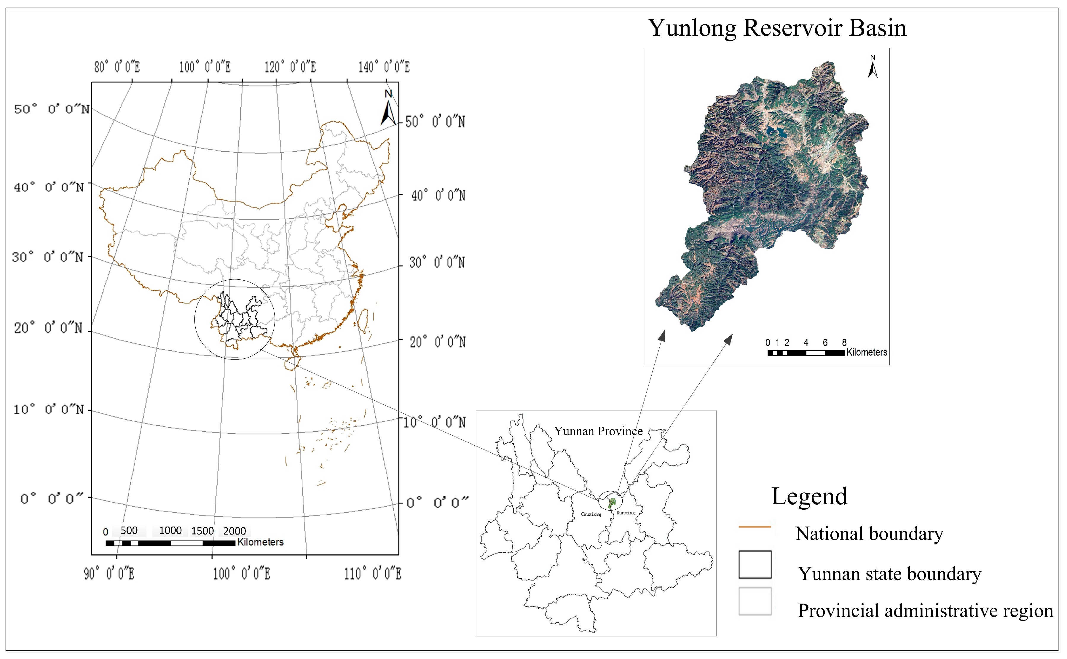
Little research has been done on integrating mixed pixel decomposition and decision trees to improve LULC classification. Therefore, this study aimed to design a methodological framework to carry out LULC classification by integrating pixel unmixing and decision tree, and a Landsat-8 OLI image of the Yunlong Reservoir Basin in Kunming, China, was used to test this proposed framework. The proposed method is provided in next section, followed by its main results and discussions in Section 3 and Section 4, and the conclusion is given at the end.

2. Data and Methods

2.1. Study Area

Yunlong Reservoir Basin (102°22′30′′~102°32′18′′E, 25°5′16′′~25°58′6′′N), with a total runoff area of 745 km2, is located in the northern Kunming City, Yunnan Province, China (Figure 1). The basin primarily belongs to a karst-tectonic origin canyon landform, a valley that was caused by mountainous tectonic erosion, and its landscape is fragmented. Yunlong Reservoir houses 70% of the total water supply for Kunming City and is responsible for maintaining sufficient drinking water for Kunming and its surrounding areas. Forest cover (including arboreal forest, shrubs, and herbs) makes up more than 70% of the basin [27].

2.2. Data Sources

2.2.1. Landsat-8 OLI Image

A Landsat-8 OLI image that was acquired on 4 August 2017 covering the study area was downloaded from the USGS Global Visualization Viewer [28]. It has seven multispectral bands with 30 m resolution (wavelength range of 0.43–2.29 um), one panchromatic band with 15 m resolution (0.50–0.68 um), and two thermal infrared bands with 100 m resolution (wavelength range of 10.6–12.51 µm).

2.2.2. Digital Elevation Model (DEM)

The DEM of study area with a resolution of 30 m was downloaded from the GloVis platform, and it is a subset of ASTER GDEM (Advanced Space borne Thermal Emission and Reflection Radiometer Global Digital Elevation Model) on 4 August 2017.

2.2.3. Ground Spectral Measurements

Ground spectral data were acquired on 4 August 2017 using an analytical spectral device (ASD) spectrometer based on field measurements, and they covered the typical spectral objects that were found in Yunlong Reservoir Basin, including coniferous forest (Yunnan pine and fir), broadleaf forest (e.g., eucalyptus trees), grassland, sparse shrub, and arable land (e.g., corn, potato, barley, and walnut).

2.2.4. LULC Classification Validation Data

603 field surveys of LULC evenly distributed across the study area were collected on 4 August 2017 for validating LULC classification, including: arable land (60 points), gardens (30 points), coniferous forest (55 points), broad-leaved forest (55 points), sparse forest (50), sparse shrub (45), medium coverage grassland (45 points), high coverage grassland (45 points), building region (43 points), roads (35 points), dams (20 points), other structures (25 points), artificial piling and digging land (25 points), revetment (25 points), desert and bare surface (25 points), and water (20 points), for a total of 16 LULC types.

2.3. Methods

The proposed methodological framework for improved decision tree classification (Figure 2) includes, mixed pixel decomposition, construction of an improved decision tree feature dataset, training sample selection based on three-dimensional (3D) Terrain, implementation of an improved decision tree, and accuracy evaluation. The basic premise of building an improved decision tree model is that (1) mixed pixel decomposition can be used to extract different endmember abundance quantities (the proportion of different kinds of features) from multispectral or hyperspectral data [29,30,31,32,33], (2) pixel unmixing can combine with classifier [34], and (3) the decision tree classification method can fuse various data features (such as terrain, texture, spectral information, Iterative Self-organizing Data Analysis Technique (ISODATA) results, Minimum Noise Fraction (MNF) results, and abundance) [35,36,37,38] Therefore, through decision tree algorithms, the potential ROI rules can be mined to establish classification tree for improving LULC analysis.

2.3.1. Mixed Pixel Decomposition

(1) Establishment of Spectral Library
The spectral reflectance values in different regions are generally different due to the different components and different influences of topography and phenology. To minimize the effects of spectral differences on decomposition accuracy, this study collected spectral data from typical objects in the study area. Environment for Visualizing Images (ENVI Version 5.3) software was used to construct spectral library, and the spectral measurements that were acquired using an ASD spectrometer were imported into ENVI. After smoothing, a typical object spectral database for the study area was built, and it was used to identify spectral curves that were in the selection of endmembers.
(2) Minimum Noise Fraction (MNF)
MNF is a linear transformation of Principal Components Analysis (PCA) with two folds. MNF transforms were used to separate noisy data and to reduce data dimensionality and the workload of subsequent processing. The correlations between any two bands were eliminated after MNF transformation, and noise was reduced [39]. Before MNF was applied, the Landsat OLI 30 m spatial resolution multispectral bands were fused with the 15 m panchromatic band, using the Gram-Schmidt (GS) fusion method. Such a fusion not only improves the spatial resolution of multi-spectral bands, but also retains the spectral information of source imagery [40,41], which may improve the accuracy and efficiency of endmember selection. In this study, the first four components of transformation results (MNF1-MNF4) were used to select endmembers due to fact that they retained 93.65% of original information.
(3) Endmember Selection
Based on the needs for this study and the available information (we found some land cover types with obvious phenomenon of mixed pixels in our study area at field investigation, especially for forest, arable land, and sparse shrub), the endmember selection method based on geometric vertex and PPI methods was adopted to select nine types of endmember objects (inclusing arboreal forest, sparse shrub, high albedo, grassland, water, arable land (including crops), arable land (no crops), low albedo, desert-, and bare surface). A fully constrained least squares mixed pixel decomposition tool was developed using Interactive data Language (IDL) for the extraction of abundance and ensuring no negative values [42]. Root Mean Square Error (RMSE) was applied to assess the accuracy of the mixed pixel decomposition results [43].

2.3.2. Construction of an Improved Decision Tree Feature Dataset

(1) Spectral Characteristics
Spectral characteristics represent the spectral information of objects in an image, and each object has specific characteristics [44]. In this study, based on the selected Landsat 8 image, several spectral characteristics were selected, including bands 1–7, Normalized Difference Vegetation Index (NDVI), Positive Vegetation Index (PVI), Ratio Vegetation Index (RVI), Enhanced Vegetation Index (EVI), Difference Vegetation Index (DVI) and the results of MNF1-MNF4 (Table 1).
(2) Texture Features
Generally, texture refers to the spatial variation of image’s hue as a function of rank, and it is defined as a clear texture area, while a gray level relative to different texture regions must be relatively close. A co-occurrence matrix was applied to extract texture features, which includes mean, variance, homogeneity, contrast, dissimilarity, entropy, second moment, and correlation (Table 2).
(3) Terrain Features
Terrain features affect the accuracy of LULC classification, especially in the regions with large topographic fluctuations [48,49]. A DEM is an important data source for terrain feature extraction, and the DEM, slope, and aspect were classified into terrain features to facilitate the construction of an improved decision tree dataset.
The improved decision tree proposed in this study incorporated five kinds of feature datasets, including ISODATA, texture, terrain, spectral characteristics and abundance of typical objects. Based on ISODATA result, DEM, slope, aspect, bands 1–7, NDVI, PVI, RVI, EVI, DVI, MNF1–MNF4, mean, variance, homogeneity, contrast, dissimilarity, entropy, second moment, and correlation, a total of 38 indicators (some of which incorporate multiple bands) were used to create an improved decision feature dataset, and the feature datasets were encoded in order to facilitate and improve the efficiency of decision tree algorithms for mining training samples (Table 3).

2.3.3. Training Sample Selection by 3D Terrain

Training sample selection (ROIs) is the most important component of most remote sensing classification methods, and assessing the quality of ROIs is also needed for improving the classification accuracy. However, the quality of ROIs is often overlooked when training samples are selected with high priori knowledge. ROI separability is often used to measure the accuracy of training samples. The ROI separability was determined by using the “Jeffries-Matusita and Transformed Divergence separability” measures, and a separability index was computed between each pair of training samples [50,51]. The values of ROI separability range from 0 to 2, and the value greater than 1.8 is often considered to be a high quality training sample [52]. Each training sample contains both spectral and pixel information. ROI separability is higher, but the correlation between the categories is lower, making it easier to distinguish between different categories and allow for classification algorithm to mine information from samples [53]. Therefore, classification accuracy is largely determined by ROI separability. However, for low or medium-resolution images and in regions with landscape fragmentation or complex terrain, ROI separability is often unsatisfactory. In this study, we proposed a new training sample selection method using a 3D terrain that was created by OLI image fusion with DEM to select ROIs, which departs from the traditional method based on a two-dimensional image.
The 3D terrain training sample selection utilizes the principle of color synthesis and integrated terrain from various angles (looking down, looking up, from top, from side) to select ROIs, and it can improve the efficiency and separability of samples to a great extent (Figure 3). In this study, the ROI separability of LULC types was greater than 1.9, and most of them reached 2.0.

2.3.4. Implementing Improved Decision Tree

Considering the “Contents and Indices of the First National Geographic Survey in Yunnan”, the actual conditions in the study area and the limited spatial resolution of Landsat OLI image, the LULC classification system of Yunlong reservoir basin was determined (Table 4).
To complete the LULC classification and accuracy assessment for the study area, 3D terrain scene was applied to select training samples of LULC types, and QUEST (Quick Unbiased Efficient Statistical Tree) [54,55,56], CRUISE (Classification Rule with Unbiased Interaction Selection and Estimation, 1D 2D) [35,57], and See5.0/C5.0 [35,58] algorithm for the decision tree were applied to mine the rules from training samples. The results that were derived from proposed improved decision tree (QUEST, CRUISE 1D, CRUISE 2D, and See5.0/C5.0) classification were compared with those of the original decision tree classification.

2.3.5. Accuracy Evaluation

Using 603 field surveys of LULC evenly distributed across the study area(Figure 4), the results derived from proposed decision tree (QUEST, CRUISE 1D, CRUISE 2D, and See5.0/C5.0) classification were compared with those of original decision tree classification to access the accuracy of the proposed method. Confusion matrix as the accuracy assessment standard, the basic precision index of overall accuracy and Kappa coefficient were used to assess the accuracy of LULC classification (Table 5).
The test is focused on the cases that are correctly classified by one classifier but misclassified by the other. With this test, two classifications may exhibit different accuracies at the 95% level of confidence, if Z > |1.96| [60].

3. Results

3.1. Mixed Pixel Decomposition

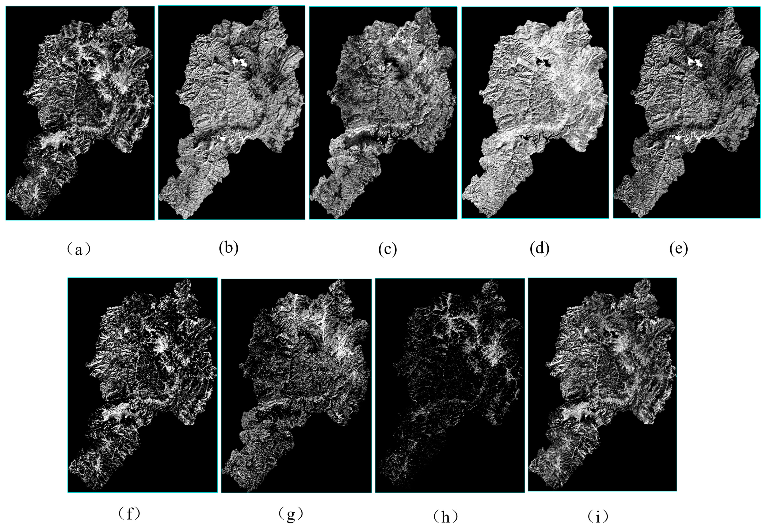
The abundance maps of nine endmembers that were derived from mixed pixel decomposition, including arboreal forest, sparse shrub, high albedo, grassland, water, arable land (including crops), arable land (no crops), low albedo, and desertand bare surface, were shown in Figure 5. Decomposition accuracy gradually increases with decreasing RMSE, and the overall RMSE error for endmember abundance was approximately 0.174913 (Table 7), which satisfied the demands of this study.

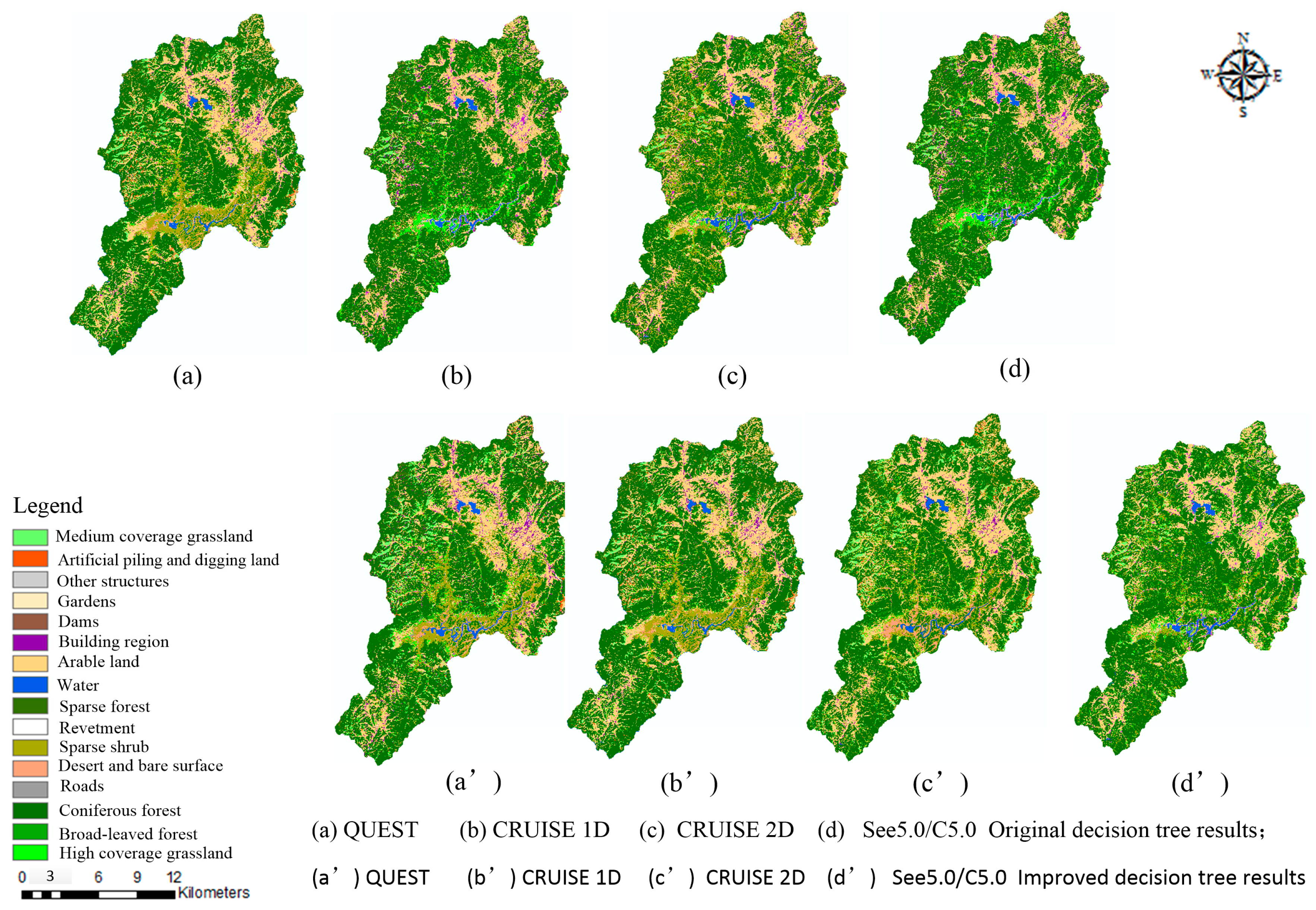
3.2. LULC Classification

Some LULC types were divided into Level 2 to Level 3 classes (Table 4), including: arable land, gardens, coniferous forest, broad-leaved forest, sparse forest, sparse shrub, medium coverage grassland, high coverage grassland, building region, roads, dams, other structures, artificial piling and digging land, revetment, desert and bare surface, and water, for a total of 16 LULC types (Figure 6).
The basic precision index of overall accuracy, user’s accuracy and Kappa coefficient were calculated, as shown in Table 8. The classification accuracy for the improved decision tree method was generally higher than that of the original decision tree (Table 8). Accuracy was gradually reduced from QUEST, CRUISE 2D, CRUISE 1D to See5.0/C5.0. Kappa coefficients, overall accuracies of the original and improved decision tree method using QUEST were more than 85%, and the improved decision tree method even reached 95%. On the contrary, the accuracies of the original decision tree method using CRUISE 2D, CRUISE 1D and See5.0/C5.0 were no more than 85%, while the improved decision tree method were more than 85%, and those results were better than those of the original decision tree method using QUEST. The Kappa coefficient and overall accuracy of the QUEST improved decision tree were 0.1% and 10%, respectively, and they were better than those of the original method. Those values also increased by 0.1% and 10% for CRUISE 1D, by 0.06% and 8% for CRUISE 2D, by 0.11% and 12% for See5.0/C5.0. Overall, the Kappa coefficients and overall accuracy of the improved decision tree method were improved by averages of 0.093% and 10%, respectively.
McNemar’s test confirmed that the improved decision tree method was significantly better than original decision tree method using QUEST (Z = 5.35, p < 0.05), CRUISE 2D (Z = 5.01, p < 0.05), CRUISE 1D (Z = 4.30, p < 0.05) and See5.0/C5.0 (Z = 4.12, p < 0.05). These results indicate that each of the proposed improved decision tree methods plays important roles in LULC classification.

3.3. Classification Error Analysis

The areas of all the LULC types that were derived from the original and improved decision tree were calculated to analyze the classification accuracy and error (Table 9). The areas for LULC types with clear spectral and texture features (arable land, coniferous forest, dams, desert and bare surface, and water) were consistent across different extraction algorithms, considering the original and improved decision tree method.
There were significant differences, however, in the areas for LULC types with spectral confusion and mixed pixels, such as sparse shrub, sparse forest, high coverage grassland, building region, other structures, and artificial piling and digging land. Clear under- or over-estimations occurred, in particular, in high coverage grassland, medium coverage grassland, and construction areas. For example, the area results from the original decision tree using QUEST, CRUISE 1D, CRUISE 2D and See5.0/C5.0 were 24.33, 10.43, 26.65 and 24.88 km2 for medium coverage grassland, and 32.44, 27.83, 27.25, and 36.77 km2 for high coverage grassland, respectively, while under the improved decision tree method, they were 34.33, 20.43, 36.65, and 34.88 km2 for low coverage grassland, and 17.44, 11.82, 10.25, and 24.77 km2 for high coverage grassland, respectively; and, on average, the area estimations for these classes were improved by nearly 10 km2. The area estimations for gardens and structures differed by an order of magnitude. While the area results from the original decision tree using QUEST and CRUISE 1D were 9.39 and 9.04 km2 for building region, but under the improved decision tree method, they were 24.38 and 12.04 km2, respectively; and on average, the area estimations for this class was improved by nearly 3 km2.

4. Discussion

We found that the improved decision tree classification method that was proposed in this study was very effective in improving LULC classification accuracy. This result may be explained by that the improved decision tree method not only combined multi-features, but also fused mixed pixel decomposition theory and introduced abundance into decision tree calculations, which has rarely been done in prior classifications. This method solved issues that the original decision tree classification for LULC types with serious spectral confusion and mixed pixels was poor, such as arboreal forest, sparse shrub, high albedo, grassland, water, arable land (including crops), arable land (no crops), low albedo, desert, and bare surface . These objects contained mixed pixels, resulting in lower classification accuracy, but for the classification of the LULC types with obvious characteristics, such as water and arable land, it was more accurate. The improved decision tree method was able to successfully classify mixed pixels, and it had high accuracy, especially in regions with fragmented landscape and complex terrain. When abundance maps were introduced into the decision tree dataset, the decision tree algorithms could better mine potential classification rules that increased the probability of identifying objects. Therefore, it was easy to identify LULC types like sparse shrub, sparse forest, grassland, construction area, other structures and artificial digging pile.
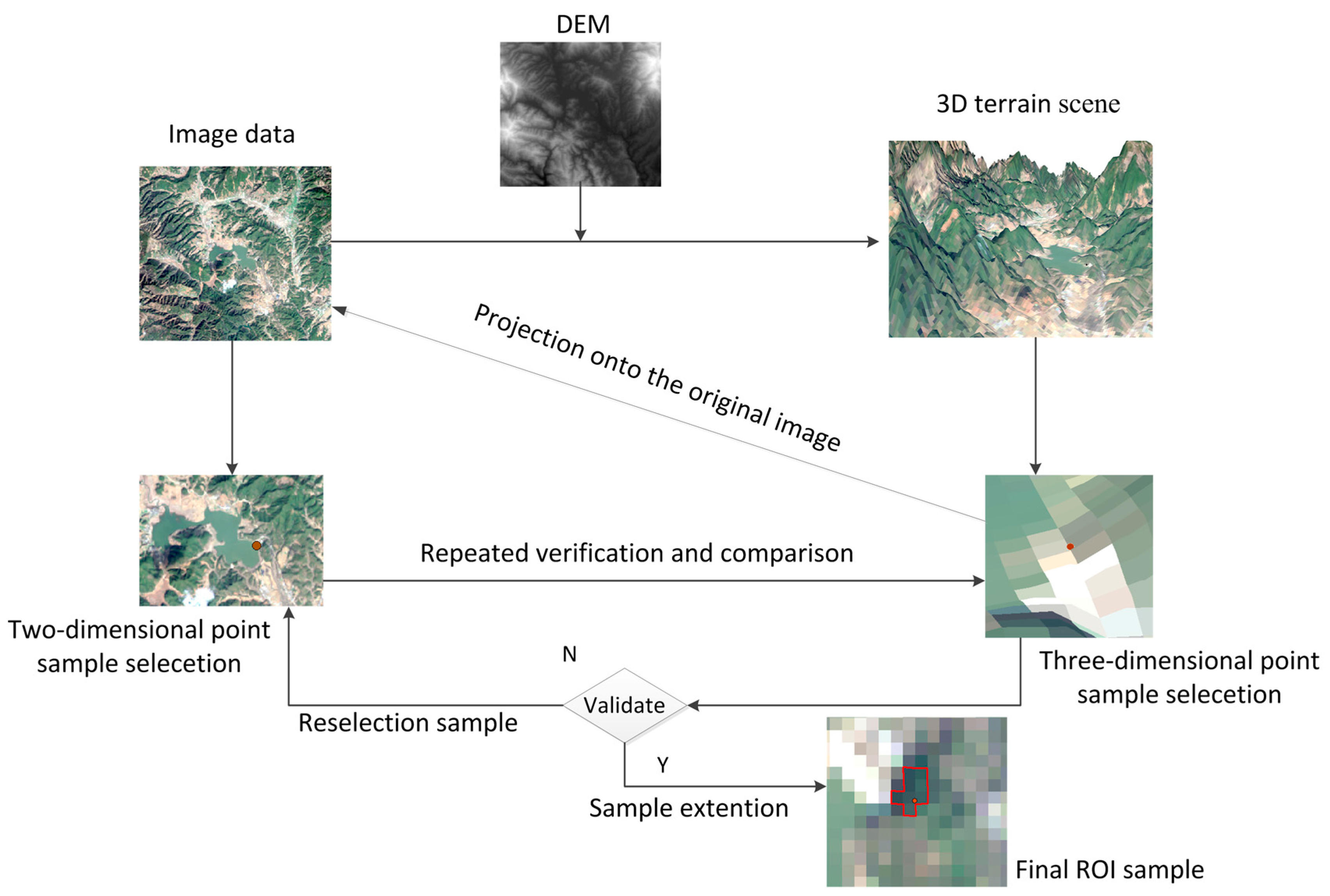
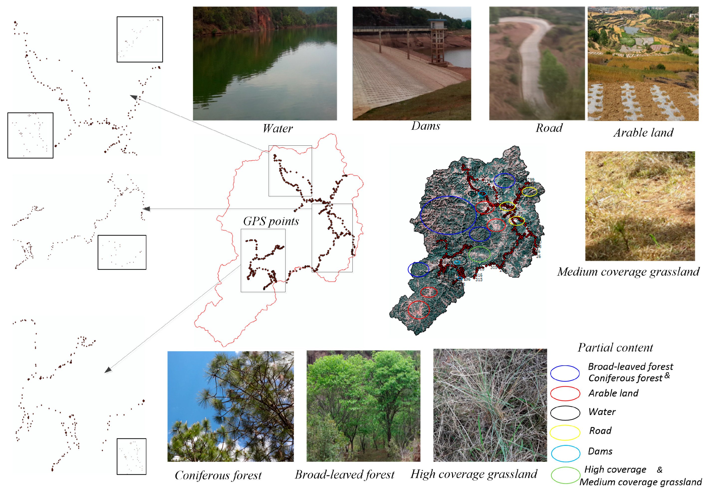
Due to the fragmented landscape and complex terrain in this study area, the traditional training sample selection method that was based on two-dimensional imagery was limited. Although it was attempted repeatedly, it was impossible to select 16 LULC types, while ensuring that their ROI separability was greater than 1.8. Unqualified training samples can reduce the classification accuracy to a large extent. To overcome this limitation, we proposed a new training sample selection method using a 3D terrain that was created by OLI image fusion DEM to select ROIs, which circumvented the traditional method that was based on a two-dimensional image. This method was not limited to the color synthesis principle, but also used different 3D angles (looking-down, looking-up, head, side-looking) to select ROIs. It allowed for us to efficiently select 16 LULC samples and to improve their ROI separability to greater than 1.9, and most of them reached 2.0. These highly qualified training samples helped improving the accuracy of subsequent classification.
Although the improved decision tree method for LULC classification that is proposed in this study was effective and obtained a high classification accuracy, only the main decision tree algorithms (QUEST, CRUISE 2D, CRUISE 1D, See5.0/C5.0) were tested, while other algorithms, such as Classification and Regression Tree (CART) and Iterative Dichotomiser 3 (ID3), were not tested. We just used linear spectral model to obtain abundance maps of nine endmembers, not using non-linear spectral model in this study. It is worthwhile to study whether non-linear spectral models can obtain better abundance of mixed pixel decomposition. We also did not compare this proposed method with other methods, such as maximum likelihood, ANN, and SVM. The future works should be carried out to simplify the decision tree dataset without affecting the classification accuracy, and to try to use additional decision tree algorithms to finalize the comparison. In addition, non-linear spectral models will be used to obtain abundance maps in this study, and the results should be compared with the linear spectral model. Besides, we will strengthen the contrast of different methods and establish an adaptive method to implement the comparative assessment of classification accuracy.

5. Conclusions

Because of the accuracy and application limitations of the traditional decision tree method, we proposed a classification method integrating decision tree classification method and mixed pixel decomposition theory, while using 3D Terrain to select training samples to improve the ROI separability. This method improved the LULC classification in the study area, and resolved the problem of distinguishing between LULC types with severe spectral confusion or clearly mixed pixels. The improved decision tree classification method was able to adapt, not only to a complex LULC classification problem, but also to other classification efforts as well, such as vegetation classification and built-up urban area extraction, making it a promising tool for future remote sensing applications.

Acknowledgments

This research was funded by the National Natural Science Foundation of China (No. 91546106) and (No. 2017YFC0506200, 2017YFC0506201). The authors thank five anonymous reviewers whose comments and suggestions greatly improved the manuscript.

Author Contributions

C.Y. conducted data analyses and prepared the manuscript; C.Y., Q.L., J.W. and G.W. developed methodology; C.Y., K.D. contributed to LULC classification; T.Z. and G.W. provided valuable insights and edited manuscript.

Conflicts of Interest

The authors declare no conflict of interest.

References

  1. Sophia, S.R.; Rwanga, J.; Ndambuki, M. Accuracy assessment of land use/land cover classification using remote sensing and GIS. Int. J. Geosci. 2017, 8, 611–622. [Google Scholar] [CrossRef]
  2. Punia, M.J.; Joshi, P.K.; Porwal, M.C. Decision tree classification of land use land cover for Delhi, India using IRS-P6 AWiFS data. Expert Syst. Appl. 2011, 38, 5577–5583. [Google Scholar] [CrossRef]
  3. Xu, C.G.; Anwar, A. Based on the decision tree classification of remote sensing image classification method application. Appl. Mech. Mater. 2013, 316, 193–196. [Google Scholar] [CrossRef]
  4. Jenkins, B.K.; Tanguay, A. Handbook of Neural Computing and Neural Networks; MIT Press: Boston, MA, USA, 1995; pp. 10–157. [Google Scholar]
  5. Han, L.Q. Artificial Neural Network; Beijing University of Posts and Telecommunications Press: Beijing, China, 2006; pp. 56–216. [Google Scholar]
  6. Dong, J.; Hu, S.X. The research progress and prospects of chaotic neural network. Inf. Control 1997, 26, 360–368. [Google Scholar] [CrossRef]
  7. Vapnik, V.N. The Nature of Statistical Leaning Theory, 2nd ed.; Springer: New York, NY, USA, 2000; pp. 10–157. [Google Scholar]
  8. Corinna, C.; Vladimir, V. Support vector networks. Mach. Learn. 1995, 20, 273–297. [Google Scholar] [CrossRef]
  9. Zadeh, L.A. Soft computing, fuzzy logic and recognition technology. In Proceedings of the IEEE World Congress on Computational Intelligence, Anchorage, AK, USA, 4–9 May 1998; pp. 1678–1679. [Google Scholar]
  10. Nuaek, D.; Kurse, R. A neuro-fuzzy method to learn fuzzy classification rules from data. Fuzzy Sets Syst. 1997, 89, 277–288. [Google Scholar] [CrossRef]
  11. Richard, O.; Duda, P.E.; Hart, D.G. Pattern Classification, 2nd ed.; China Machine Press: Beijing, China, 2004; pp. 192–195. [Google Scholar]
  12. Li, C.K.; Fang, W.; Dong, X.J. Research on the classification of high resolution image based on object-oriented and class rule. Int. Arch. Photogramm. Remote Sens. 2015, XL, 75–80. [Google Scholar] [CrossRef]
  13. Benz, U.C.; Hofmann, P.; Willhauck, G.; Lingenfelder, I.; Heynen, M. Multi-resolution, object-oriented fuzzy analysis of remote sensing data for GIS-ready information. ISPRS J. Photogramm. Remote Sens. 2004, 58, 239–258. [Google Scholar] [CrossRef]
  14. Zhang, Y.; Zhang, J.; Huang, G.; Zhao, Z. Object-Oriented classification of Polarimetric SAR imagery based on texture features. Int. Symp. Image Data Fusion 2011. [Google Scholar] [CrossRef]
  15. Friedl, M.A.; Brodley, C.E. Decision tree classification of land cover from remotely sensed data. Remote Sen. Environ. 1997, 61, 399–409. [Google Scholar] [CrossRef]
  16. Simard, M.; Saatchi, S.S.; Grandi, G.D. The use of decision tree and multi-scale texture for classification of JERS-1 SAR data over tropical forest. IEEE Trans. Geosci. Remote Sens. 2000, 38, 2310–2321. [Google Scholar] [CrossRef]
  17. Pavuluri, M.K.; Ramanathan, S.; Daniel, Z. A rule-based classifier using classification and regression tree (CART) approach for urban landscape dynamics. In Proceedings of the Geoscience and Remote Sensing Symposium, Toronto, ON, Canada, 24–28 June 2002; pp. 24–28. [Google Scholar]
  18. Dai, E.; Zhuo, W.U.; Haihua, L.U.; Hua, F.U. Linear spectral unmixing-based method for the detection of land cover change in Naidong County, Qinghai-Tibet Plateau. Prog. Geogr. 2015, 34, 854–861. [Google Scholar] [CrossRef]
  19. Charles, I.; Arnon, K. A review of mixture modeling techniques for sub-pixel land cover estimation. Remote Sens. Rev. 1996, 13, 161–186. [Google Scholar] [CrossRef]
  20. Roberts, D.A.; Gardner, M.; Church, R.; Ustin, S.; Scheer, G.; Green, R.O. Mapping chaparral in the Santa Monica Mountains using multiple end member spectral mixture mode. Remote Sens. Environ. 1998, 65, 267–279. [Google Scholar] [CrossRef]
  21. Rashed, T.; Weeks, J.R.; Gadalla, M.S.; Hill, A.G. Revealing the anatomy of cities through spectral mixture analysis of multispectral satellite imagery: A case study of the Greater Cairo Region, Egypt. Geocarto Int. 2001, 16, 5–16. [Google Scholar] [CrossRef]
  22. Rashed, T.; Weeks, J.R. Measuring the physical composition of urban morphology using multiple end-member spectral mixture models. Photogramm. Eng. Remote Sens. 2003, 69, 1011–1020. [Google Scholar] [CrossRef]
  23. Smith, M.O.; Ustin, S.L.; Adams, J.B.; Gillespie, A.R.; Smith, M.O. Vegetation in deserts: I. A regional measure of abundance from multispectral images. Remote Sens. Environ. 1990, 31, 1–26. [Google Scholar] [CrossRef]
  24. Roberts, D.A.; Smith, M.O.; Adams, J.B. Green vegetation, non-photosynthetic vegetation, and soil in AVIRIS. Remote Sens. Environ. 1993, 44, 255–269. [Google Scholar] [CrossRef]
  25. Xu, N.; Hu, Y.X.; Lei, B.; Zhang, C.; Wang, D.M.; Shi, T. Automated mineral information extraction based on PPI algorithm for hyperspectral imagery. Sci. Surv. Mapp. 2013, 38, 138–141. [Google Scholar] [CrossRef]
  26. Chang, C.I.; Plaza, A. A fast iterative algorithm for implementation of pixel purity index. IEEE Geosci. Remote Sens. Lett. 2006, 3, 63–67. [Google Scholar] [CrossRef]
  27. Liu, W.G.; Tang, F.L.; Liu, S.J. The southwest drought on different forest vegetation watershed-taking Songhuaba Reservoir and Yun Long Reservoir as an example. For. Econ. 2012, 10, 12–17. [Google Scholar]
  28. United State Geological Survey. GloVis. Available online: https://glovis.usgs.gov/ (accessed on 4 August 2017).
  29. Xu, M.; Du, B.; Zhang, L. Spatial-spectral information based abundance-constrained endmember extraction methods. J. Sel. Top. Appl. 2014, 7, 2004–2015. [Google Scholar] [CrossRef]
  30. Wu, J.C.; Tsuei, G.C. Comparison of hyperspectral endmember extraction algorithms. J. Appl. Remote Sens. 2013, 7, 073525. [Google Scholar] [CrossRef]
  31. Weng, F.; Pu, R. Mapping and assessing of urban impervious areas using multiple endmember spectral mixture analysis: A case study in the city of Tampa, Florida. Geocarto Int. 2013, 28, 594–615. [Google Scholar] [CrossRef]
  32. Nie, M.; Liu, Z.; He, X.; Qiu, Q.; Zhang, Y. End-member extraction based on segmented vertex component analysis in hyperspectral images. Appl. Opt. 2017, 56, 2476–2480. [Google Scholar] [CrossRef] [PubMed]
  33. Heylen, R.; Parente, M.; Scheunders, P. Estimation of the number of endmembers in a hyperspectral image via the Hubness phenomenon. IEEE Trans. Geosci. Remote Sens. 2017, 99, 1–10. [Google Scholar] [CrossRef]
  34. Dópido, I.; Li, J.; Gamba, P.; Plaza, A. A new hybrid strategy combining semisupervised classification and unmixing of hyperspectral data. IEEE J. Sel. Top. Appl. Earth Obs. Remote Sens. 2014, 7, 3619–3629. [Google Scholar] [CrossRef]
  35. Quinlan, J.R. Induction on decision tree. Mach. Learn. 1986, 1, 81–106. [Google Scholar] [CrossRef]
  36. Rajeswari, K.; Preeti, K. Selection of significant features using decision tree classifiers. Preeti Kumari Int. J. Eng. Res. Appl. 2014, 4, 48–51. [Google Scholar]
  37. Racoviteanu, A.; Williams, M.W. Decision tree and texture analysis for mapping debris-covered glaciers in the Kangchenjunga area, Eastern Himalaya. Remote Sens. 2012, 4, 3078–3109. [Google Scholar] [CrossRef]
  38. Landgrebe, D. A survey of decision tree classifier methodology. IEEE Trans. Syst. Man Cybern. 2002, 21, 660–674. [Google Scholar] [CrossRef]
  39. Guan, L.; Xie, W.; Pei, J. Segmented minimum noise fraction transformation for efficient feature extraction of hyperspectral images. Pattern Recogn. 2015, 48, 3216–3226. [Google Scholar] [CrossRef]
  40. Yang, C.; Wang, J.L.; Qu, L.Q.; Li, S.H.; Sun, X.Q. Research on the extraction of surface feature abundance based on the least square mixed pixel decomposition. Sci. Surv. Mapp. 2017, 229, 147–158. [Google Scholar]
  41. Li, C.J.; Liu, L.Y.; Wang, J.H.; Wang, R.C. Comparison of Two Methods of Fusing Remote Sensing Images with Fidelity of Spectra Information. In Proceedings of the Geoscience and Remote Sensing Symposium, Anchorage, AK, USA, 20–24 September 2004; pp. 1376–1385. [Google Scholar]
  42. Heinz, D.C.; Chang, C. Fully constrained least squares linear spectral mixture analysis method for material quantification in hyperspectral imagery. IEEE Trans. Geosci. Remote Sens. 2002, 39, 529–545. [Google Scholar] [CrossRef]
  43. Zhang, F.F.; Sun, X.; Xue, L.Y.; Gao, L.R.; Liu, C.X. Hyperspectral mixed pixel decomposition policy merging simple linear iterative clustering. Trans. CSAE 2015, 31, 199–206. [Google Scholar] [CrossRef]
  44. Myneni, R.B.; Hall, F.G. The interpretation of spectral vegetation indexes. IEEE Trans. Geosci. Remote Sens. 1995, 33, 481–486. [Google Scholar] [CrossRef]
  45. Halounová, L. Reclamation areas and their development studied by vegetation indices. Int. J. Digit. Earth 2008, 1, 155–164. [Google Scholar] [CrossRef]
  46. Zhao, Y.S. Principles and Methods of Analysis of Remote Sensing Applications; Science Press: Beijing, China, 2003; pp. 1–206. [Google Scholar]
  47. Dai, C.D. Remote Sensing Image Application Processing and Analysis; Tsinghua University Press: Beijing, China, 2004; pp. 45–187. [Google Scholar]
  48. Vanonckelen, S.; Lhermitte, S.; Rompaey, A.V. The effect of atmospheric and topographic correction methods on land cover classification accuracy. Int. J. Appl. Earth Obs. 2013, 24, 9–21. [Google Scholar] [CrossRef]
  49. Moreira, E.P.; Valeriano, M.M. Application and evaluation of topographic correction methods to improve land cover mapping using object-based classification. Int. J. Appl. Earth Obs. 2014, 32, 208–217. [Google Scholar] [CrossRef]
  50. Richards, J.A.; Jia, X. Remote Sensing Digital Image Analysis: An Introduction, 3rd ed.; Springer: New York, NY, USA, 2006; pp. 47–54. [Google Scholar]
  51. Sunil, B.; Shanka, P.; Maria, R. Per-pixel and object-oriented classification methods for mapping urban features using Ikonos satellite data. Appl. Geogr. 2010, 4, 650–665. [Google Scholar] [CrossRef]
  52. Zhu, X.F.; Pan, Y.; Zang, J.S.; Wang, S.; Gu, X.H.; Xu, C. The effects of training samples on the wheat planting areameasure accuracy in TM scale (I): The accuracy response of different classifiers to training samples. J. Remote Sens. 2007, 6, 826–836. [Google Scholar]
  53. Jin, H.; Stehman, S.V.; Mountrakis, G. Assessing the impact of training sample selection on accuracy of an urban classification: A case study in Denver, Colorado. Int. J. Remote Sens. 2014, 35, 2067–2081. [Google Scholar] [CrossRef]
  54. Bag, M.; Gauri, S.K.; Chakraborty, S. Feature-based decision rules for control charts pattern recognition: A comparison between CART and QUEST algorithm. Int. J. Ind. Eng. Comput. 2012, 3, 199–210. [Google Scholar] [CrossRef]
  55. JianSheng, W.U.; Pan, K.Y.; Peng, J.; Huang, X.L. Research on the accuracy of TM images land-use classification based on QUEST decision tree: A case study of Lijiang in Yunnan. Geogr. Res. 2012, 31, 1973–1980. [Google Scholar]
  56. Duan, H.; Deng, Z.; Deng, F. Classification of groundwater potential in Chaoyang area based on QUEST algorithm. In Proceedings of the Geoscience and Remote Sensing Symposium (IGARSS), Beijing, China, 10–15 July 2016; pp. 890–893. [Google Scholar]
  57. Kim, H.; Loh, W.Y. Classification trees with unbiased multi-way splits. J. Am. Stat. Assoc. 2001, 96, 589–604. [Google Scholar] [CrossRef]
  58. Bai, X.; Wuliangha, B.; Hasiqiqige. The study of the remote sensing image classification based on C5.0 algorithm of decision tree. Remote Sens. Technol. Appl. 2014, 29, 338–343. [Google Scholar]
  59. Foody, G.M. Thematic map comparison: Evaluating the statistical significance of differences in classification accuracy. Photogramm. Eng. Remote Sens. 2004, 70, 627–633. [Google Scholar] [CrossRef]
  60. Shi, T.; Liu, J.Z.; Hu, J.; Liu, H.; Wang, J.; Wu, G.F. New spectral metrics for mangrove forest identification. Remote Sens. Lett. 2016, 9, 885–894. [Google Scholar] [CrossRef]
Figure 1. Location of Yunlong Reservoir Basin.
Remotesensing 09 01222 g001
Figure 2. Methodological framework for proposed improved decision tree method. The abundance data derived from mixed pixel decomposition as the most important features together with other features to establish multi-feature dataset for decision tree, then using a three-dimensional (3D) Terrain model to select training samples (ROIs) of land use/land cover (LULC), finally decision tree algorithms (QUEST, CRUISE, See5.0/C5.0) were used to mine potential ROIs rules of LULC, and complete LULC classification.
Remotesensing 09 01222 g002
Figure 3. The flow chart of 3D terrain-aided ROI selection.
Remotesensing 09 01222 g003
Figure 4. GPS points for LULC analysis in the study area.
Remotesensing 09 01222 g004
Figure 5. Endmember abundance maps of mixed pixel unmixing, (a) Grassland abundance, (b) Water abundance, (c) Arable land (including crops) abundance, (d) Arboreal forest abundance, (e) Low albedo abundance, (f) Arable land (no crops) abundance, (g) Desert and bare surface abundance, (h) High albedo abundance, and (i) Sparse shrub abundance. The range of abundance values is 0–1, and the brighter (values closer to 1) indicates the greater probability of approaching pure pixel.
Remotesensing 09 01222 g005
Figure 6. Land use/land cover classification results derived from the original and improved decision tree, respectively.
Remotesensing 09 01222 g006
Table 1. Expression and characteristic table of vegetation index [44,45,46,47].
Vegetation IndexExpressionIndex Characteristics
NDVI N D V I = ρ N I R ρ R E D ρ N I R + ρ R E D The range of NDVI values is [−1, 1], the greater the NDVI value, the more green vegetation cover there is.
PVI P V I = 0.939 ρ N I R 0.344 ρ R E D + 0.09 PVI can better eliminate the influence of soil in background.
RVI R V I = ρ N I R ρ R E D The value of RVI is greater than 1 for green healthy vegetation, while on a non-vegetated land surface (bare soil, water bodies, artificial buildings, serious disease, and insect pests or a vegetation dead zone), the RVI value is near 1. RVI is usually greater than 2.
EVI E V I = 2.5 ( ρ N I R ρ R E D ρ N I R + 6 ρ R E D 7.5 ρ B L U E + 1 ) EVI can correct for the influence of soil background and aerosol scattering. The range of values is [−1, 1], and green vegetation is generally [0.2–0.8].
DVI D V I = ρ N I R ρ R E D DVI is extremely sensitive to changes in soil background.
Note: ρ N I R , ρ R E D and ρ B L U E represent the reflectance in near infrared, red and blue regions, respectively.
Table 2. A commonly used model for texture characteristics [46,48].
NumberFeature NameExpression Model
1Mean M E = i , j = 0 n 1 i × P i , j
2Variance V A = i , j = 0 n 1 i × P i , j ( i M E ) 2
3Homogeneity H O = i , j = 0 n 1 i × p i , j 1 + ( i j ) 2
4Contract C O = i , j = 0 n 1 i × p i , j ( 1 j ) 2
5Dissimilarity D I = i , j = 0 n 1 i × p i , j | i j |
6Entropy E N = i , j = 0 n 1 i × p i , j ( Ln p i , j )
7Second Moment S M = i , j = 0 n 1 i × p i , j 2
8Correlation C R = i , j = 0 n 1 i × p i , j [ ( i M E ) ( j M E ) V A i × V A j ]
Note: p i , j = V i , j i , j = 0 n 1 V i j , V i , j represents the pixel brightness value at column j of line i, and n represents the size of the moving window when calculating each texture measure.
Table 3. Feature dataset of improved decision tree.
EncodeFeature DataEncodeFeature Data
B1OLI1B20Arable land (including crops) abundance
B2OLI2B21Arable land (no crops) abundance
B3OLI3B22Desert and bare surface abundance
B4OLI4B23High albedo abundance
B5OLI5B24Sparse shrub abundance
B6OLI6B25Arboreal forest abundance
B7OLI7B26Low albedo abundance
B8MNF1B27DEM
B9MNF2B28Slop
B10MNF3B29Aspect
B11MNF4B30Other topographic elements
B12ISODATAB31Mean
B13NDVIB32Variance
B14PVIB33Homogeneity
B15RVIB34Contract
B16EVIB35Dissimilarity
B17DVIB36Entropy
B18Grassland abundanceB37Second moment
B19Water abundanceB38Correlation
Table 4. LULC classification system used in this study.
First ClassSecond ClassThird Class
1 farming land12 arable land-
2 garden--
3 forest land31 arbor forest311 broad-leaved forest
312 coniferous forest
32 sparse forest-
33 sparse shrub-
4 grassland41 natural grassland411 high coverage grassland
412 medium coverage grassland
5 building region--
6 roads--
7 structure71 hardened surface711 revetment
72 hydraulic facilities721 dams
73 other structures-
8 artificial piling and digging land--
9 desert and bare surface--
10 water--
Note: “-” for classification only to the upper class in this study, not divided into “-” types.
Table 5. Precision index of LULC classification.
NumberPrecision IndexExpression Model
1Overall accuracy p o = i = 1 n N i i / N
2Kappa coefficient K a p p a = N i = 1 n N i i - i = 1 n ( N i + N + i ) N 2 i = 1 n ( N i + N + i )
n and N represent the number of classes, and the total number of samples, respectively. Nii, Ni+ and N+i represent the correctly classified pixel, the sum of the class i in the classified data, and the sum of class i in the validation data, respectively. The statistical significance of the difference between classifications was evaluated using McNemar’s test [59,60]. This non-parametric test is based on a binary distinction between correct and incorrect class allocations (Table 6). McNemar’s test is also based on the standardized normal test statistic, expressed as following Equation:
Z = f 12 f 21 f 12 + f 21 .
Table 6. Assessment of the statistical significance between two classifications using McNemar’s test.
Classification 2
Allocation CorrectIncorrect
Classification 1Correctf11f12
Incorrectf21f22
f12, the test pixels that are correctly classified by classification 1 but misclassified by classification 2; f21, the test pixels that are correctly classified by classification 2 but misclassified by classification 1.
Table 7. Root Mean Square Error (RMSE) error.
Endmember Abundance CombinationRMSE ErrorRMSE Mean Value
Grassland, water, arable land (including crops)RMSE10.174913
Arboreal forest, high albedo, sparse shrubRMSE20.174913
Arboreal forest, low albedo, arable land (including crops)RMSE30.174914
Low albedo, desert and bare surface, arable land (no crops)RMSE40.174913
Table 8. Accuracy comparison derived from the original and improved decision tree, respectively.
AlgorithmsKappa CoefficientOverall AccuracyAlgorithmsKappa CoefficientOverall Accuracy
Original decision treeQUEST0.840987.84% Improved decision treeQUEST0.951996.26%
CRUISE 1D0.757281.69% CRUISE 1D0.862189.55%
CRUISE 2D0.811185.81% CRUISE 2D0.897192.14%
See5.0/C5.00.740579.36% See5.0/C5.00.849588.52%
Table 9. Area comparison using the original and improved decision tree. Unit: (km2).
LULC TypesOriginal Decision TreeImproved Decision Tree
QUESTCRUISE 1DCRUISE 2DSee5.0/C5.0QUESTCRUISE 1DCRUISE 2DSee5.0/C5.0
Arable land154.15163.50169.40162.00154.18163.70169.47162.03
Garden1.082.102.010.771.283.103.011.77
Coniferous forest350.29381.53379.21361.97356.29381.53379.14361.99
Broad-leaved forest26.2911.9410.3822.5220.2611.9410.3822.48
Sparse forest39.6745.9233.5330.6127.6734.9226.5320.60
Sparse shrub66.8755.6170.8650.0376.8765.4176.8659.04
Medium coverage grassland24.3310.4326.6524.8834.3320.4336.6534.88
High coverage grassland32.4427.8327.2536.7717.4411.8210.2524.77
Building region19.399.048.067.6024.3812.048.759.59
Roads6.8510.281.477.586.8613.291.487.59
Dams0.160.180.080.080.140.180.080.09
Revetment0.950.700.161.780.970.750.161.77
Other structure3.475.402.124.891.463.340.112.87
Artificial piling and digging land3.486.082.869.715.498.094.8711.73
Desert and bare surface11.359.2912.6418.5511.339.2412.5418.45
Water6.976.105.536.176.996.155.636.27
Total745.94745.93745.91745.92745.94745.93745.91745.92

