Article

A Hyperspectral Imaging Approach to White Matter Hyperintensities Detection in Brain Magnetic Resonance Images

1
Center for Quantitative Imaging in Medicine (CQUIM), Department of Medical Research, Taichung Veterans General Hospital, Taichung 40705, Taiwan
2
Department of Biomedical Engineering, Hungkuang University, Taichung 43302, Taiwan
3
Department of Radiology, Taichung Veterans General Hospital, Taichung 40705, Taiwan
4
College of Medicine, China Medical University, Taichung 40402, Taiwan
5
Remote Sensing Signal and Image Processing Laboratory, Department of Computer Science and Electrical Engineering, University of Maryland, Baltimore County, Baltimore, MD 21250, USA
6
School of Physics and Optoelectronic Engineering, Xidian University, Xi’an 710126, China
7
Center for Hyperspectral Imaging in Remote Sensing (CHIRS), Information and Technology College, Dalian Maritime University, Dalian 116026, China
8
State Key Laboratory of Integrated Services Networks, Xi’an 710071, China
9
Department of Computer Science and Information Engineering, National Yunlin University of Science and Technology, Yunlin 64002, Taiwan
10
Department of Computer Science and Information Management, Providence University, Taichung 43301, Taiwan
*
Author to whom correspondence should be addressed.
Remote Sens. 2017, 9(11), 1174; https://doi.org/10.3390/rs9111174
Submission received: 4 September 2017 / Revised: 9 November 2017 / Accepted: 13 November 2017 / Published: 16 November 2017
(This article belongs to the Special Issue Hyperspectral Imaging and Applications)

Abstract

:
White matter hyperintensities (WMHs) are closely related to various geriatric disorders including cerebrovascular diseases, cardiovascular diseases, dementia, and psychiatric disorders of elderly people, and can be generally detected on T2 weighted (T2W) or fluid attenuation inversion recovery (FLAIR) brain magnetic resonance (MR) images. This paper develops a new approach to detect WMH in MR brain images from a hyperspectral imaging perspective. To take advantage of hyperspectral imaging, a nonlinear band expansion (NBE) process is proposed to expand MR images to a hyperspectral image. It then redesigns the well-known hyperspectral subpixel target detection, called constrained energy minimization (CEM), as an iterative version of CEM (ICEM) for WMH detection. Its idea is to implement CEM iteratively by feeding back Gaussian filtered CEM-detection maps to capture spatial information. To show effectiveness of NBE-ICEM in WMH detection, the lesion segmentation tool (LST), which is an open source toolbox for statistical parametric mapping (SPM), is used for comparative study. For quantitative analysis, the synthetic images in BrainWeb provided by McGill University are used for experiments where our proposed NBE-ICEM performs better than LST in all cases, especially for noisy MR images. As for real images collected by Taichung Veterans General Hospital, the NBE-ICEM also shows its advantages over and superiority to LST.

1. Introduction

White matter hyperintensities (WMHs) are commonly observed on T2W or FLAIR brain MR images of elderly people and related to various geriatric disorders including cerebrovascular diseases, cardiovascular diseases, dementia, and psychiatric disorders [1]. According to [2], WMHs are brain lesions that generally show up as brighter areas and can be visualized by T2W and FLAIR MRI sequences. It is also referred to as Leukoaraiosis and is often found in computed tomography (CT) or MRI of older patients. It is a marker of small-vessel vascular disease. In clinical practice, it is indicative of cognitive and emotional dysfunction, particularly in the ageing population. Its initial discovery was observed in the late 1980s by Hachinski and colleagues [2] who described WMH as patchy low attenuation in the periventricular and deep white matter. Since then, detection of WMH has received considerable interest. Although a supervised method may produce better results, it requires human intervention which is very time-consuming and also suffer the issues of intra- and inter-observer variation [3]. Accordingly, segmentation of WMH has been recently directed to semi-unsupervised and automatic methods which rely on computer assisted tools to help diagnosis to avoid human subjective interpretation. Most importantly, such computer assisted diagnosis can be further used to quantify WMH and calculate its volume [3,4,5,6,7]. However, it also comes with two major issues. One is that most works are based on T1 weighted (T1W), T2W and photon density (PD) or FLAIR images to produce spatial statistics to segment WMH. The other is selection of an appropriate threshold, which ultimately determines the detection results of WMH. Generally, such automatic method is not fully automatic but rather semi-unsupervised because it requires adaptively adjusting threshold values by visual inspection. This paper takes a quite different approach to designing a joint spectral–spatial method that takes advantage of spectral properties provided by MR image sequences to perform subvoxel detection in conjunction with a Gaussian spatial filter to capture spatial contextual information surrounding the WMH detected voxels.
One of the strengths of magnetic resonance imaging (MRI) is its ability in imaging structures of soft tissues. Because an MR image is collected by specifically designed image sequences such as T1W, T2W or PD, it can be considered as a multispectral image [8]. Hyperspectral imaging has recently emerged as an advanced technique in remote sensing to deal with many issues that cannot be resolved by multispectral imaging, specifically, subpixel target detection and mixed pixel classification [9]. Its applications to MRI classification have been also explored in [10,11,12,13,14,15]. However, it seems that using the concept of hyperspectral imaging techniques for WMH detection in brain MRI has not been investigated. This paper presents a new application of hyperspectral imaging in WMH detection of MR brain images.
To expand capability of multispectral imaging to hyperspectral imaging in data analysis, it suffers from insufficient band dimensionality. To resolve this dilemma, a nonlinear band expansion (NBE) process was previously proposed in [16] which used nonlinear functions to produce a new set of nonlinear band images that can be incorporated into the original images to create a new data set. As more such nonlinearly generated images are included, the resulting multispectral image has become a hyperspectral image. In this case, we can take advantage of the well-known hyperspectral subpixel target detection technique, called constrained energy minimization (CEM) [9,17,18,19], to detect the lesion of interest [20]. However, the nonlinearly expanded band images by NBE used in [20] can only capture spectral information nonlinearly but not spatial information. As noted above, effectively detecting the boundary of a lesion may also require spatial information due to the shape of the boundary that is closely related to spatial correlation.
This paper develops a novel NBE approach that expands NBE [20] to produce new band images that can capture not only nonlinear spectral information but also spatial information. Since CEM is a pixel-based technique and does not take into account spatial information. In order for CEM to capture spatial information an iterative version of CEM, to be called Iterative CEM (ICEM), is developed for this purpose. Its idea is to apply a Gaussian filter to a CEM-detection map so that the Gaussian-filtered CEM detection map will contain spatial information to be further fed back as a new band image to create a new image cube. The same process of operating CEM on this new data cube is repeated over again in an iterative manner via feedback loops. To terminate ICEM an automatic stopping rule is also designed, which uses Otsu’s method [21] to threshold the Gaussian-filtered CEM detection map obtained at each iteration as a binary image. If the two consecutive binary images agree within an error threshold measured by Dice similarity index (DSI) [22], then ICEM is terminated and the final Otsu’s thresholded binary image is the desired lesion detection map.
There are several main contributions derived from NBE-ICEM. One is using NBE to create new band images to make a multispectral image a hyperspectral image. Another is including Gaussian filters to capture spatial information. Thirdly, such Gaussian-filtered spatial information is further fed back to be included in the data cube being processed as new images to account for spatial information of detected WMH lesions. Fourthly, the spatial information included in CEM is increased via repeated feedback loop in an iterative manner. That is, the more feedbacks the more spatial information to be included in the data cube for better boundary detection. Fifthly, Otsu’s method is introduced to automatically terminate the iterative process carried out by ICEM. Finally, once the ICEM is terminated, the resulting Otsu’s thresholded binary image is the desired final lesion detection result.

2. Methods

2.1. Nonlinear Band Dimensionality Expansion

An early attempt to expand the original set of band images is to utilize nonlinear functions, for example, auto-correlation and cross-correlation, an idea derived from [16,20]. This type of NBE process is referred to as correlation band expansion process (CBEP). Combining these new CBEP-generated band images with the original set of band images produces a hyperspectral image with sufficient band images.
The CBEP presented in this section is an NBE process using correlation functions to generate new band images from the original set of multispectral images. Its original idea was developed in [16,20].
Correlation Band Expansion Process (CBEP)
Step 1. First-order band image: { B l } l = 1 L = set of original band images
Step 2. Second-order correlated band images:
(i)
{ B l 2 } l = 1 L = set of auto-correlated band images
(ii)
{ B k B l } k = 1 , l = 1 , k l L , L = set of cross-correlated band images
Step 3. Third order correlated band images
(i)
{ B l 3 } l = 1 L = set of auto-correlated band images
(ii)
{ B k 2 B l } k = 1 , l = 1 , l k L , L = set of two cross-correlated band images
(iii)
{ B k B l B m } k = 1 , l = 1 , m = 1 , k l m L , L , L = set of three cross-correlated band images
Step 4. Other nonlinear correlated band images
(i)
{ B l } l = 1 L = set of band images stretched out by the square-root.
(ii)
{ log ( B l ) } l = 1 L = set of band images stretched out by the logarithmic function.
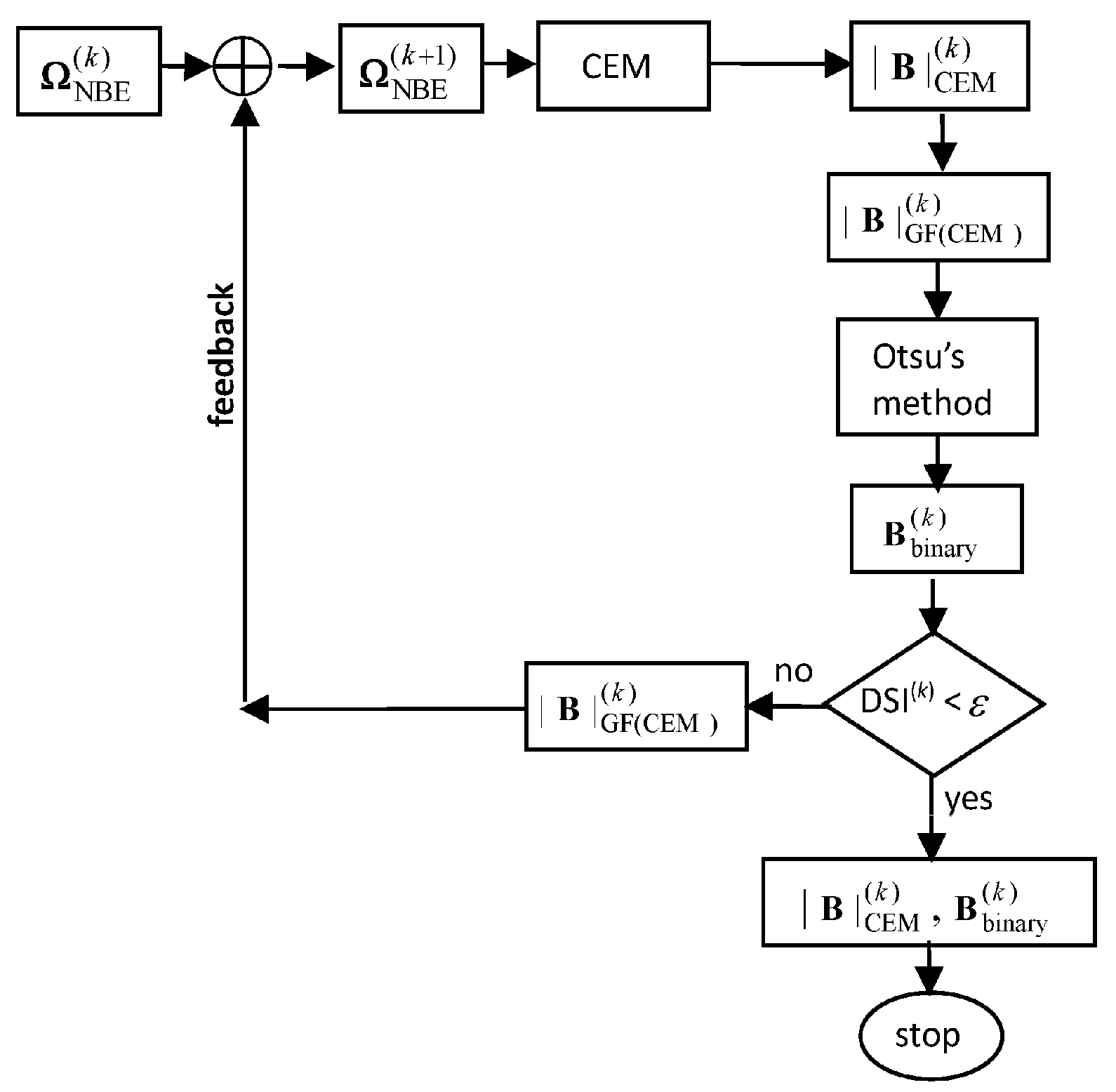
It should be noted that, according to the nonlinear functions described in Steps (1)–(4), the band images generated by CBEP contain only nonlinear spectral information but not spatial information. In what follows, we develop an iterative CEM (ICEM) to address this issue where spatial information can be captured by using a Gaussian filter and feed it back to expand images currently being processed to create a new set of image data cubes.

2.2. Iterative CEM

ICEM, presented in this section, is implemented in conjunction with CBEP in an iterative manner. More specifically, it utilizes CBEP to create new band images via an NBE process. Once CBEP process is completed, a new set of image data cubes is generated for CEM to perform subpixel target detection. To obtain class spatial information, a Gaussian filter is introduced in the CEM-detected maps so that spatial contextual information of data sample vectors can be captured by a Gaussian filter. The resulting Gaussian-filtered CEM-detection abundance fractional map is fed back to create a new band incorporated into NBE to form a new hyperspectral cube which will be further used for re-processing CEM again. The same process is repeated over and over again until a stopping rule is satisfied. This repeated implementation of CEM via feedback loops in an iterative fashion is ICEM.
Specifically, at each iteration, say kth iteration, a Gaussian filter is used to blur | B | CEM ( k ) which is the absolute value of CEM-detection abundance fractional map, B CEM ( k ) . This Gaussian-filtered band image, | B | GF ( CEM ) ( k ) provides spatial classification information as similar filters used in [23] and will be further fed back to Ω NBE ( k ) to create a new set of hyperspectral images, Ω NBE ( k + 1 ) = Ω NBE ( k ) { | B | GF ( CEM ) ( k ) } to be used by CEM again for next iteration. The same procedure is continued. To terminate the process, an automatic stopping rule is designed. It applies Otsu’s method [21] to | B | GF ( CEM ) ( k ) to produce a binary classification map, B binary ( k ) that will be used to calculate DSI [22]. If two consecutive DSI values are within an error threshold, ICEM will be terminated and | B | CEM ( k ) and B binary ( k ) will be the desired final real-valued WMH lesion detection map for visual inspection and binary value detection maps of WMH lesions for quantitative analysis.
In the following, we describe detailed step-by-step implementation of ICEM in great detail.
ICEM
  • Initial condition: Let { B l } l = 1 L be the original set of band images.
  • Use an NBE process to create a new set of nonlinear band images, { B i NB } i = 1 n NB where nNB is the number of new band images by the NBE process.
  • Form a new set of band images, Ω ( 0 ) = { B l } l = 1 L { B i NB } i = 1 n NB . Let d ( 0 ) = ( d 1 , , d L , d 1 NB , , d n NB NB ) T be the desired target pixels in Ω ( 0 ) . Let δ 0 CEM be CEM using d(0) and R(0) which are obtained from Ω ( 0 ) . Let k = 1 .
  • At the kth iteration, update d ( k ) and R ( k ) = i = 1 N r i ( k ) ( r i ( k ) ) T from Ω ( k ) .
  • Use new generated d(k) and R(k) for δ k CEM to be implemented on Ω ( k ) . Let B CEM ( k ) be the detection abundance fractional map produced by δ k CEM .
  • Use a Gaussian filter to blur | B | CEM ( k ) where | B | CEM ( k ) is the absolute value of B CEM ( k ) . The resulting image is denoted by Gaussian-filter | B | GFCEM ( k ) .
  • Check if | B | k CEM satisfies a given stopping rule. If no, continue. Otherwise, go to Step 9.
  • Form Ω ( k + 1 ) = Ω ( k ) { | B | GFCEM ( k ) } . Let k k + 1 and go to Step 4.
  • B CEM ( k ) is the desired detection abundance fractional map and ICEM is terminated.
Figure 1 delineates how ICEM is processed as a detector where ICEM uses Gaussian filters to smooth CEM-detection abundance fractional maps and feeds back Gaussian-filtered CEM detection abundance fractional maps to provide spatial information for re-processing CEM iteratively. By gradually increasing more spatial information through feedback loops the boundaries of WMH lesions can be detected more effectively. It should also be noted that, if a particular NBE technique is used such as CBEP, then NBE-ICEM can be specified by CBEP-ICEM.

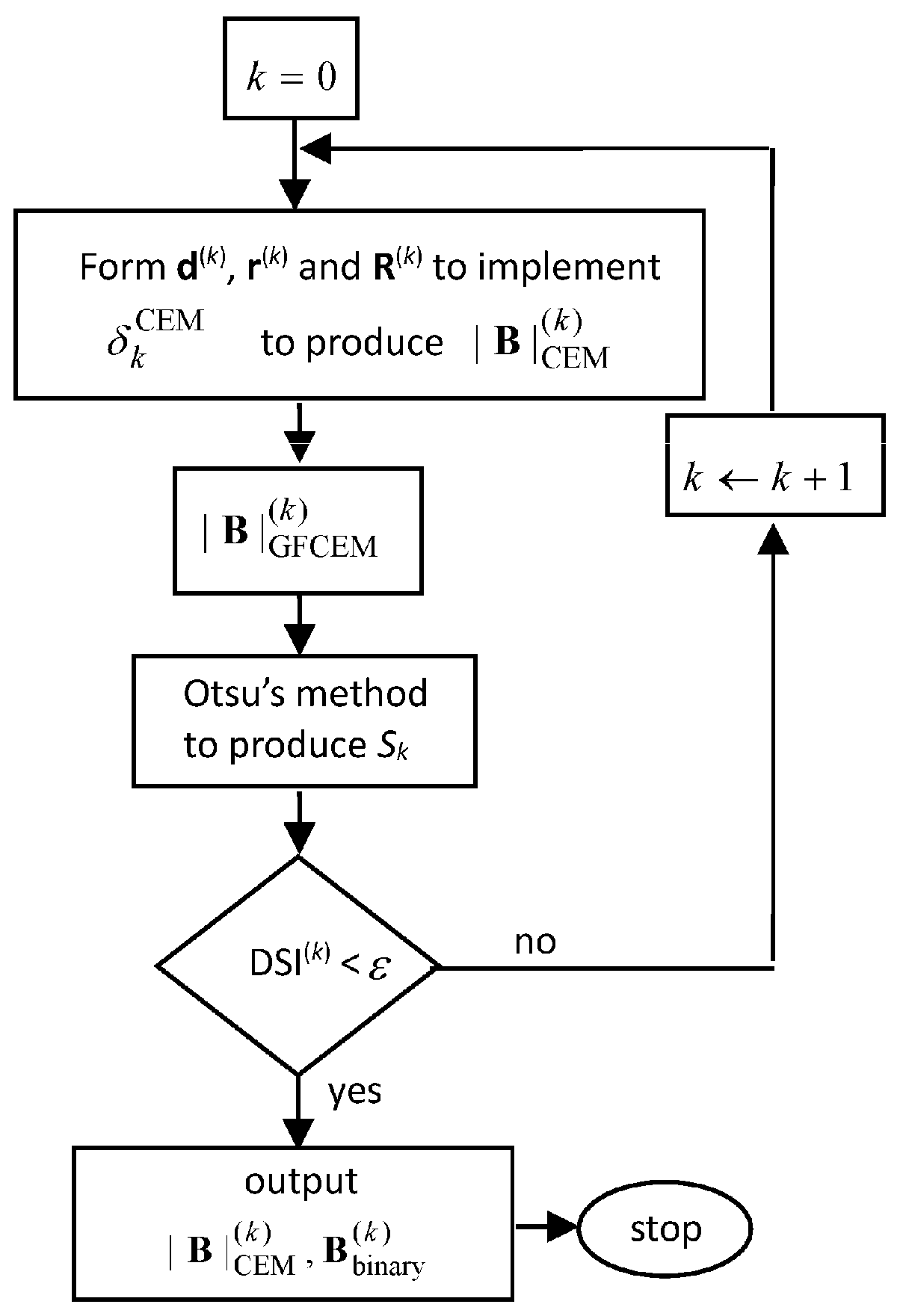
2.3. Stopping Rule for ICEM

To effectively terminate ICEM, DSI defined in [22] as
DSI ( k ) = 2 | S k S k 1 | | S k S k 1 |
is used a stopping criterion where |S| is size of a set S, Sk and Sk−1 are the kth thresholded binary image of the kth CEM detection abundance fractional map, | B | k CEM and k − 1st thresholded binary image of the k − 1st CEM detection abundance fractional map, | B | k 1 CEM . Figure 2 depicts a flow chart of a stopping rule using DSI with ε as a prescribed error threshold.

2.4. Algorithm for NBE-ICEM

Using Figure 1 and Figure 2, an algorithm developed to implement ICEM in conjunction with NBE can be described as follows. Figure 3 describes a graphic flow chart of implementing NBE-ICEM.
NBE-ICEM
  • Initial conditions:
    • For each class, find its sample mean to calculate the desired signature d for the particular class.
    • Select the values of the parameter σ used for Gaussian filters in ICEM,
    • Prescribe an error threshold ε for DSI in Equation (1)
  • Use the NBE process described in Section 2.1 to generate a set of nonlinear band images, { B l NB } l = 1 n NB .
  • Apply ICEM described in Figure 1 to Ω ( 0 ) = { B l } l = 1 L { B l NB } l = 1 n NB .
  • Use DSI described in Figure 2 as a stopping rule to terminate ICEM.
  • Output | B | CEM ( k ) , which is real-valued, and B binary ( k ) , which is binary-valued, to produce a confusion matrix for classification.

3. Results

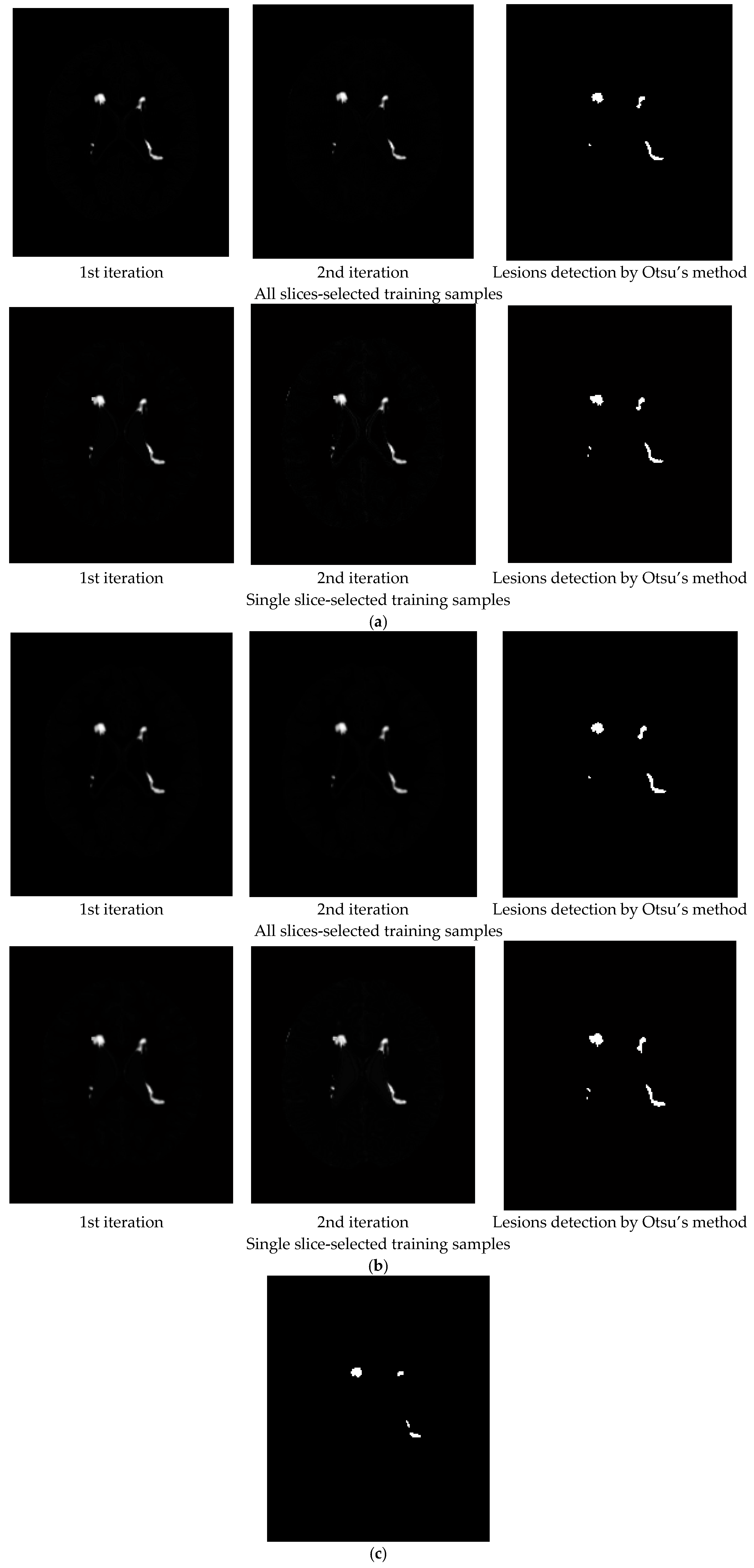
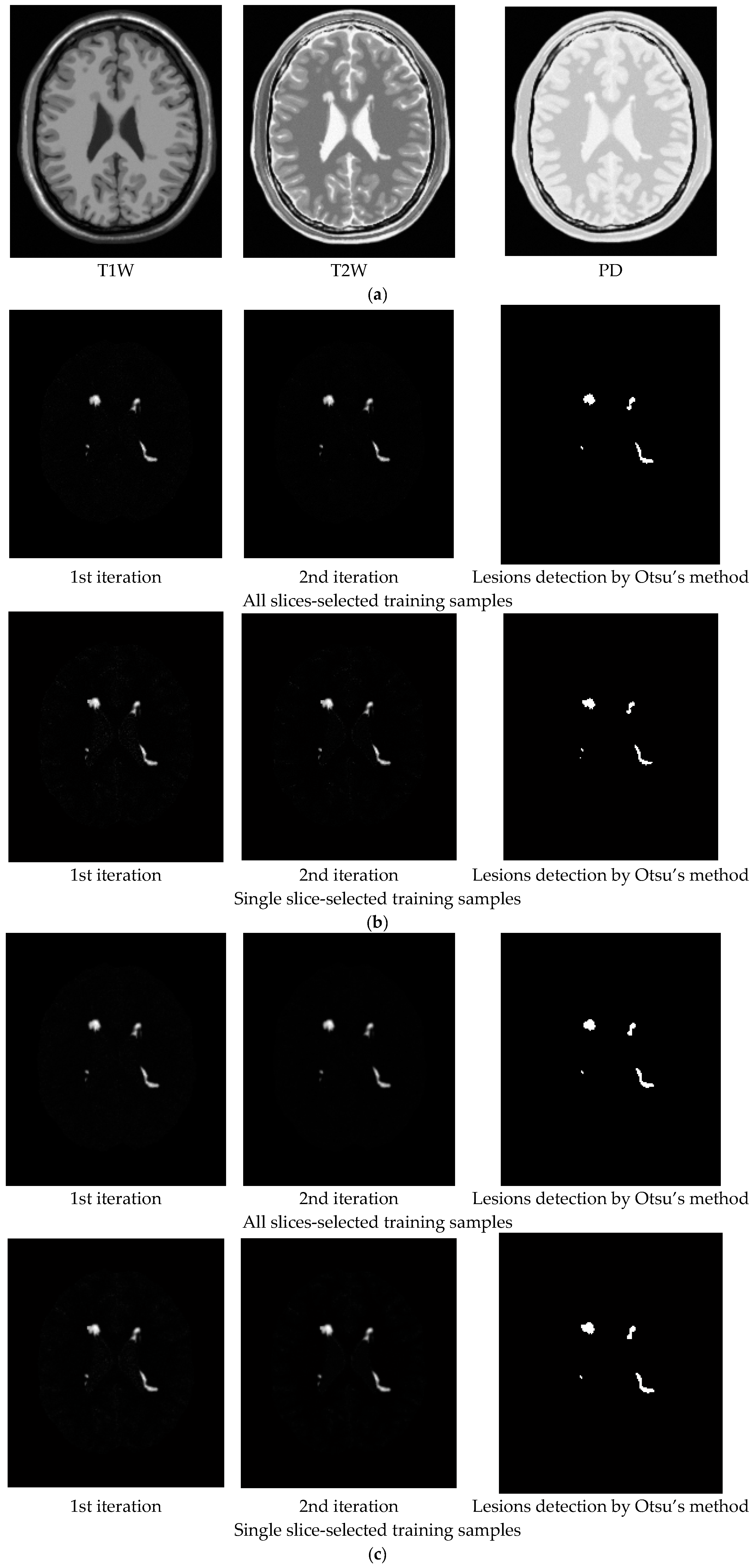
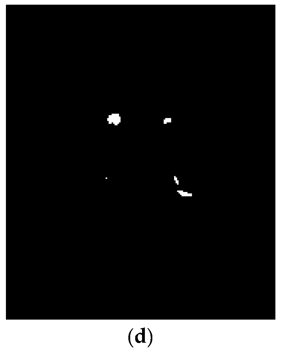
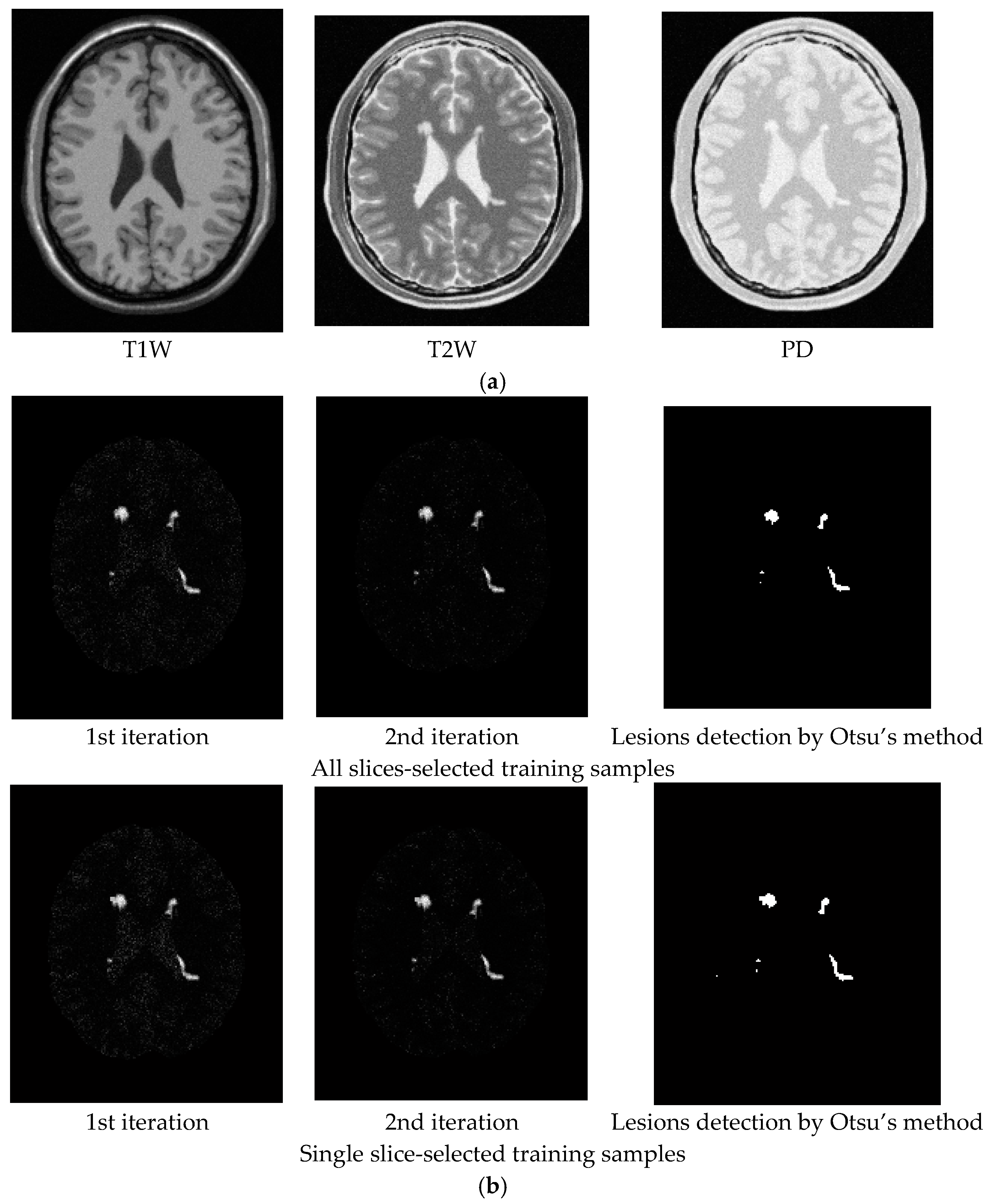
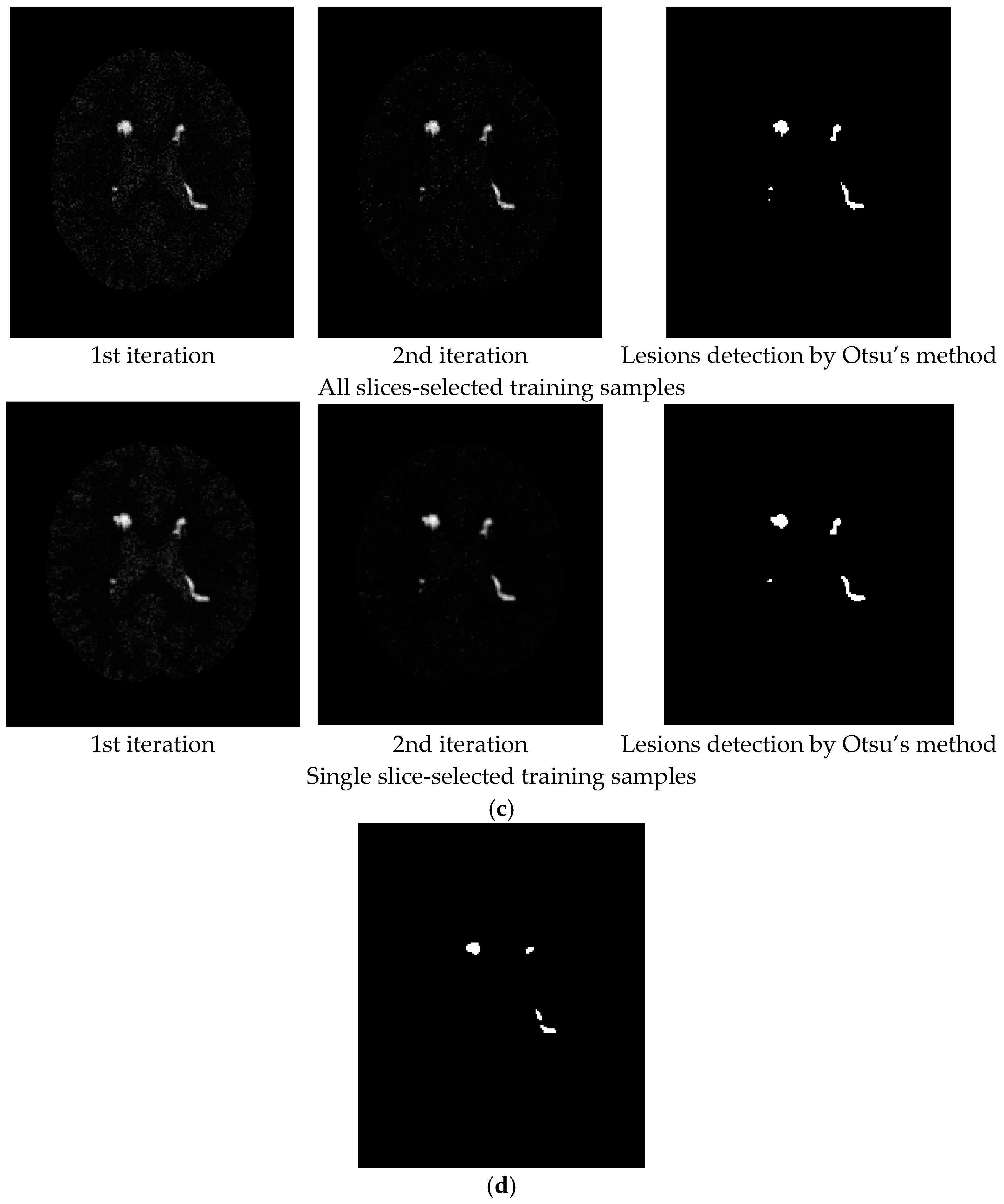
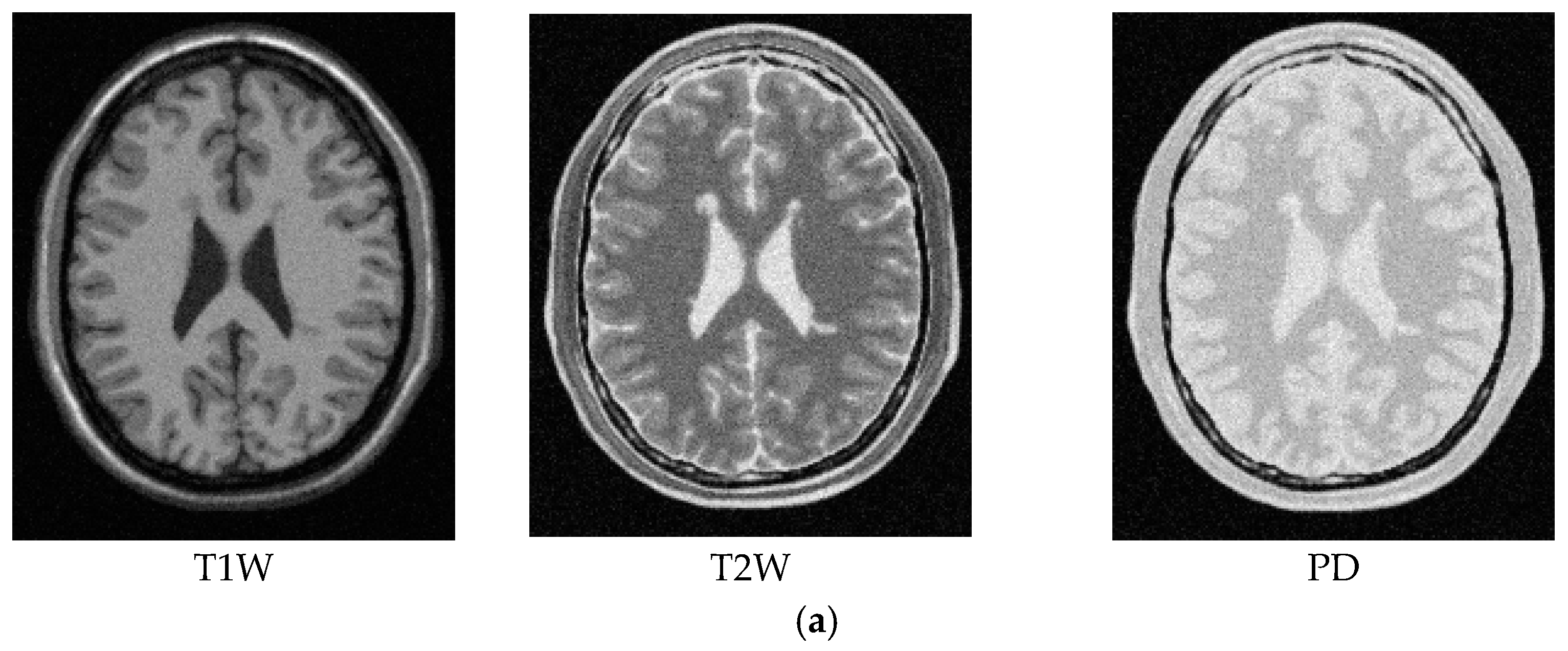
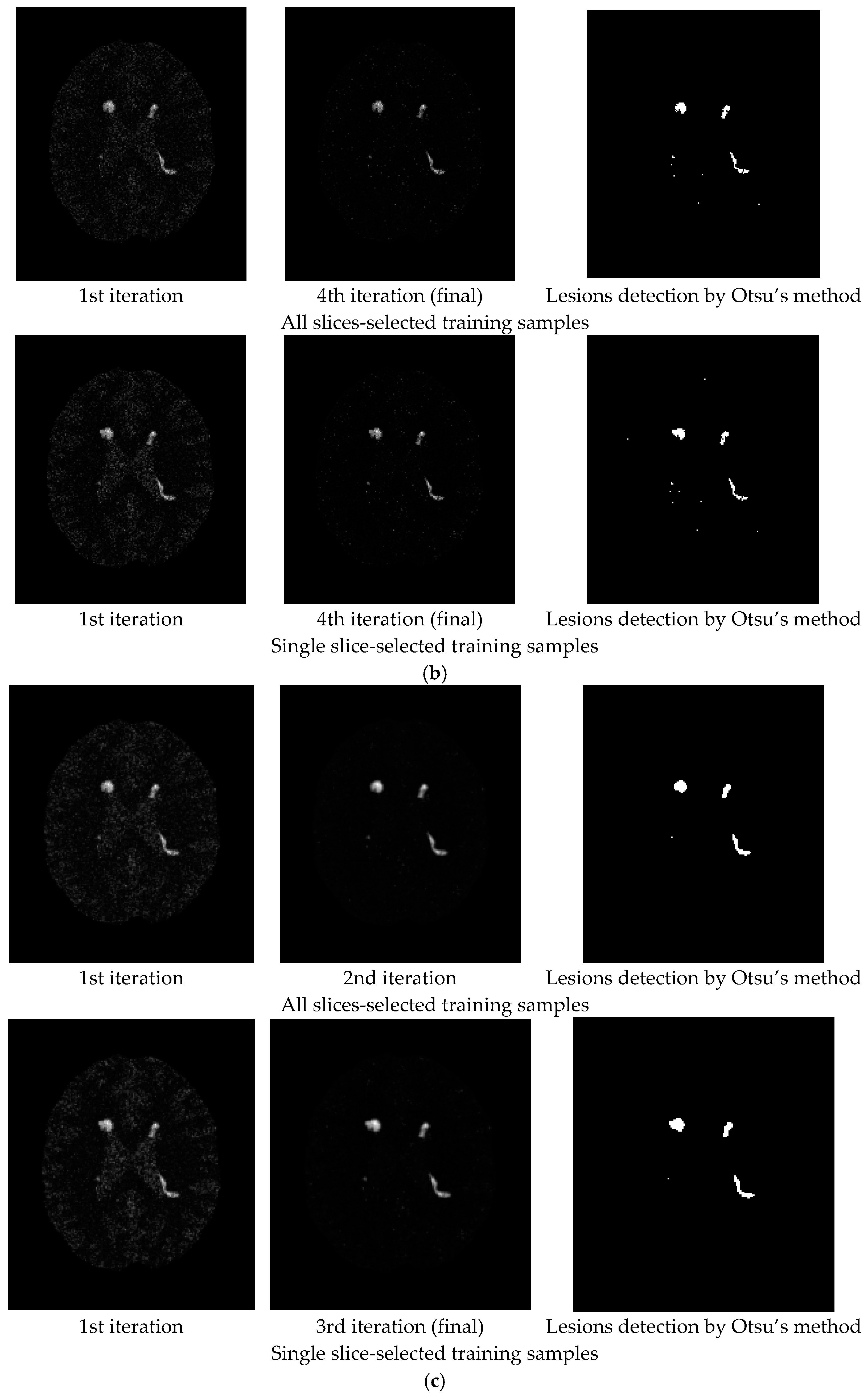
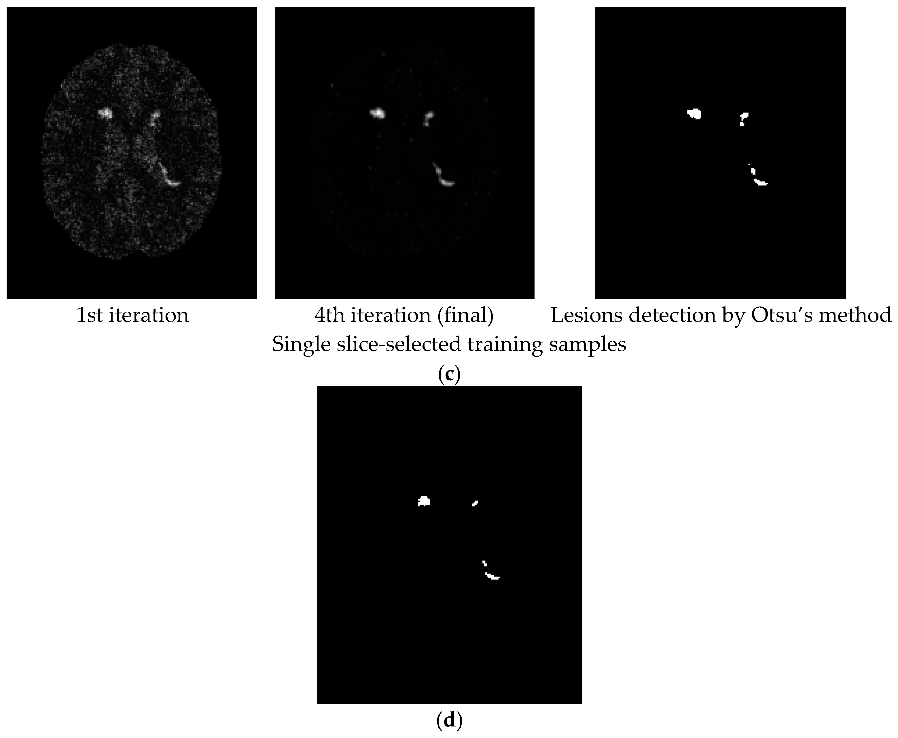
3.1. Synthetic Image Experiments

To conduct an objective quantitative study, the synthetic MR brain images containing multiple sclerosis (MS) lesions obtained from the MR imaging simulator of McGill University, Montreal, Canada were used for experiments [24]. MS lesions are typically hyperintense on T2W or FLAIR sequence image. Figure 4a–c shows a slice MR brain image along with the ground truth of MS lesion shown in Figure 4d. The MR brain images are acquired by the modalities of T1W, T2W and PD with specifications provided in BrainWeb site [24]. The thickness of slice is 1 mm with size of 181 × 217 × 181 . Each slice is specified by INU (intensity non-uniformity) 0% or 20%, denoted by rf0 and rf20 with six different levels of noise, 0%, 1%, 3%, 5%, 7% and 9%. The noise in the background of the simulated images is simulated by Rayleigh statistics and signal regions are simulated by Rician statistics. The “percentage (%) of noise” represents the ratio of the standard deviation of the white Gaussian noise to the signal for a reference tissue [24] in terms of %. There were 23 MR images from 91 to 113 slices for our study. To implement ICEM, we need to know the desired target signature d. Two ways were suggested to select training samples to calculate d. One is called all slices-selected training samples, which selects a small set of training samples from all MR image slices. The other is called single slice-selected training samples, which selects a small set of training samples from a particular single MR image slice that can be further used to find training samples for entire MR image slices. Its idea was derived from the extrapolation process used in volume sphering analysis (VSA) developed in [14,15]. Table 1 specifies the values of parameters used for experiments where two Gaussian filters using window sizes of 3 × 3 and 5 × 5 , and two different σ = 0.1 and 0.5. The experiments were conducted for all MR image slices according to Table 1 where the results obtained by Gaussian window of 5 × 5 with σ = 0.5 are tabulated in parentheses.
To further evaluate the performance of the proposed NBE-ICEM, a commonly used segmentation approach, called lesion segmentation tool (LST) [25,26], was used for comparative study. It was originally developed for the segmentation of MS lesions and has also been proven to be useful for the segmentation of brain lesions. Table 2 tabulates DSI values calculated by Equation (1) averaged over 23 MR image slices 91–113 of lesion detection produced by CBEP-ICEM1, CBEP-ICEM2 and LST for six different noise levels and two INU levels where all slices-selected training samples were used to find the knowledge of d. The shaded DSI values in Table 2 are the best results. As we can see from the table, CBEP-ICEM1 performed better than CBEP-ICEM2 when noise level is low. However, when noise level is high, CBEP-ICEM2 performed better than CBEP-ICEM1. Nonetheless, both NBE-ICEM-based methods, i.e., CBEP-ICEM1 and CBEP-ICEM2, performed better than LST. It should be also noted that, since LST produced real-valued gray scale images, it required a threshold value to segment WMH lesions. The LST results in Table 2 were obtained by manually adjusting threshold values in order to yield the highest detection rate.
Similarly, Table 3 also tabulates DSI values calculated by Equation (1) averaged over 23 MR image slices 91–113 of lesion detection produced by CBEP-ICEM1, CBEP-ICEM2 and LST for six different noise levels and two INU levels where single slice-selected training samples were used to find the knowledge of d and the slice 102 was chosen as the desired single slice. The selection of slice 102 is empirical as long as it includes sufficient tissue information, in which case the middle MR image slice can serve as this purpose. The same conclusions drawn from Table 2 were also valid for Table 3, even though the results in Table 3 were slightly degraded compared to the results in Table 2 because the single slice-selected training samples were used. It should be noted that the results of LST in Table 2 and Table 3 were the same because LST did not allow users to select training samples. This disadvantage is further offset by a need of finding an appropriate threshold value to segment lesion out from the background.
For an illustrative purpose, Figure 5, Figure 6, Figure 7, Figure 8, Figure 9 and Figure 10 only show detection results of WMH lesions of the 97th MR image slice with six levels of noise and 0% INU by two versions of CBEP-ICEM, using the Gaussian window size of 3 × 3 specified by σ = 0.1 and the Gaussian window size of 5 × 5 specified by σ = 0.5, referred to as CBEP-ICEM1 and CBEP-ICEM2, respectively, where two sets of training samples selected by all slices and the single 102nd slice were used to calculate the desired target signatures d to implement NBE-ICEM. As we can see by visual inspection against the ground truth in Figure 4d, CBEP-ICEM1 and CBEP-ICEM2 using two sets of training samples, i.e., all slices-selected and single slice-selected training samples, produced very close results and they both also performed better lesion detection than LST did.
Two comments are noteworthy.
  • Despite the fact that the training samples used for our proposed NBE-ICEM were selected based on 2D images such as by all slices and a single slice, these training samples were either stacked as voxels from all slices or extrapolated from a single slice as voxels by VSA. Accordingly, NBE-ICEM is actually run on 3D images as image cubes.
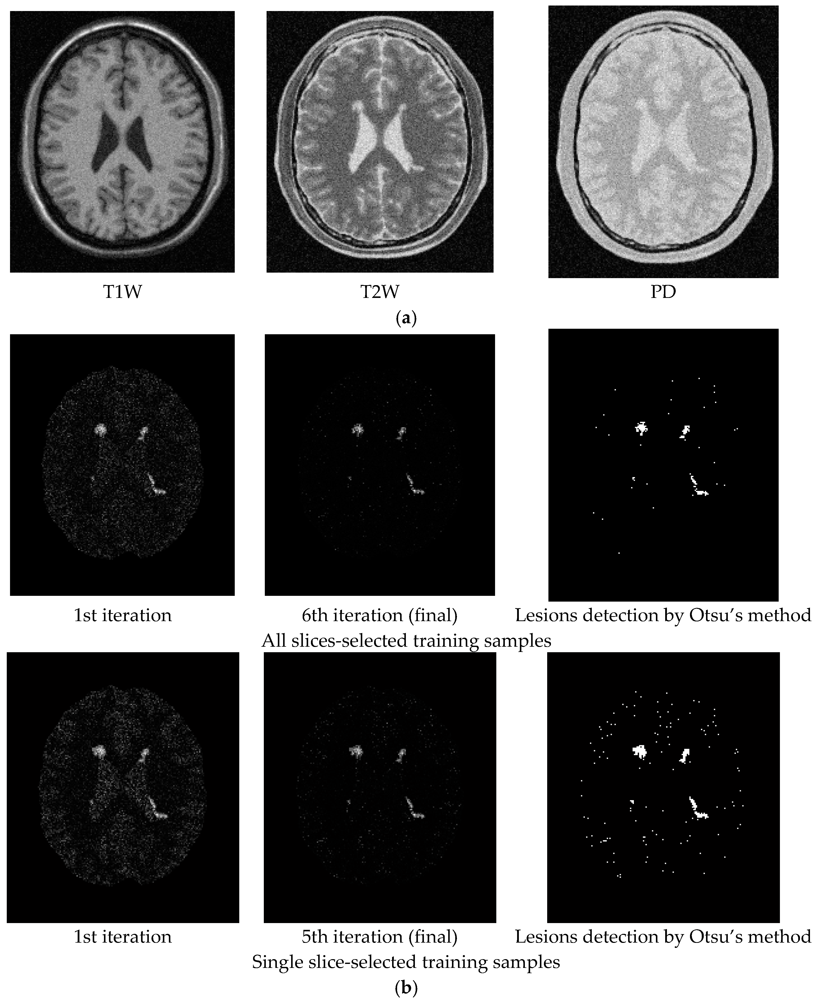
  • There is an issue in implementing LST. Since it is packaged as a software algorithm, there is no flexibility for users to choose parameters at their discretion. Besides, it cannot implement T1W, T2W or FLAIR images alone. Instead, it must require T1W images as reference images to segment WMHs [26]. Most importantly, it produces real valued gray level images, which require users selecting a threshold value from a range from 0.05 to 0.95 with a step size of 0.05 to detect WMHs. In [26], this threshold value was suggested between 0.25 and 0.4. However, in practical applications, the best value is generally selected manually. Thus, technically speaking, LST is not fully automatic. Specifically, when synthetic images from the BainWeb were used for experiments, it was found that using both T1W and T2W could not segment WMHs. It must use T1W and PD to detect WMHs and the threshold value must be set to around 0.2 to segment WMHs.

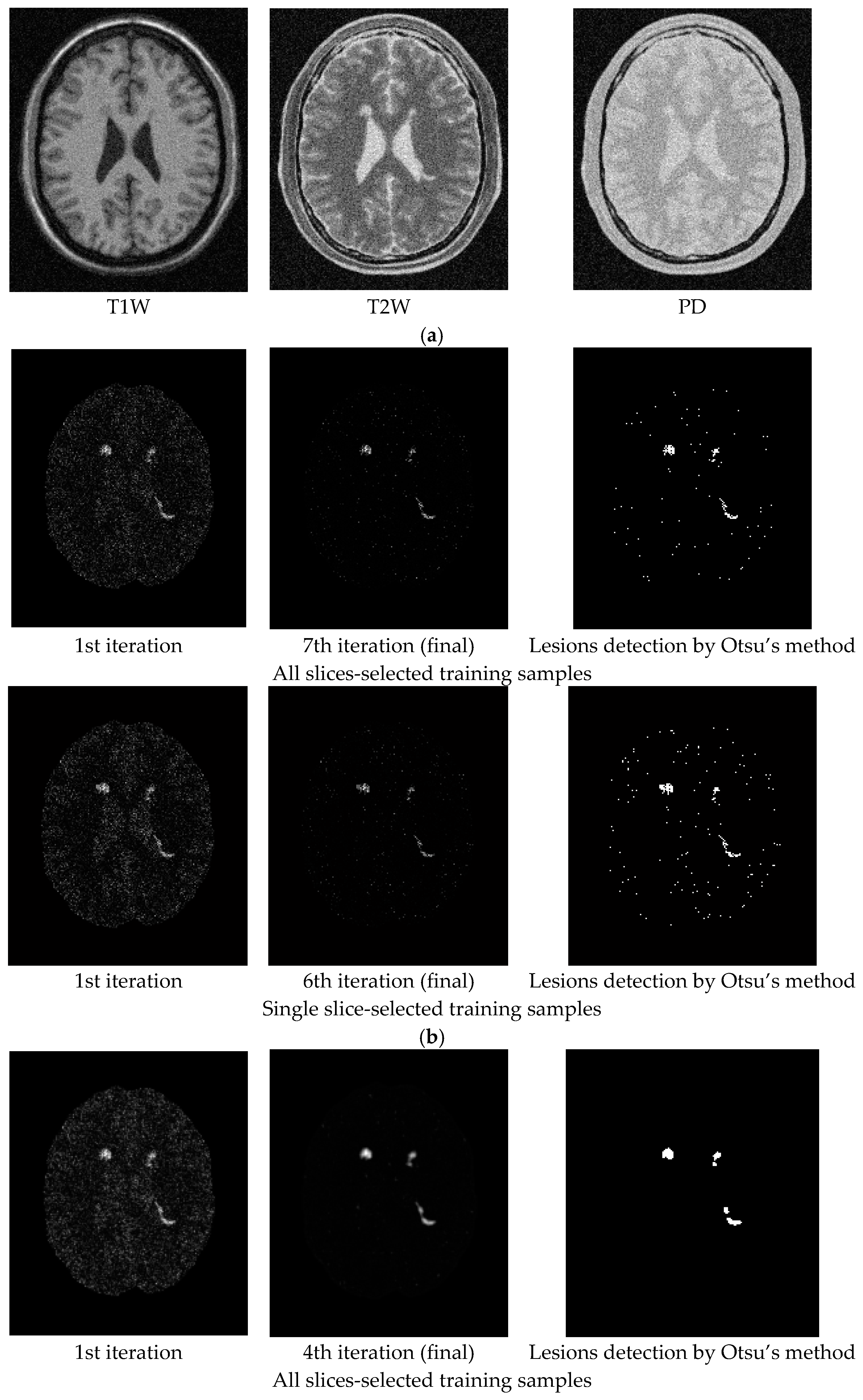
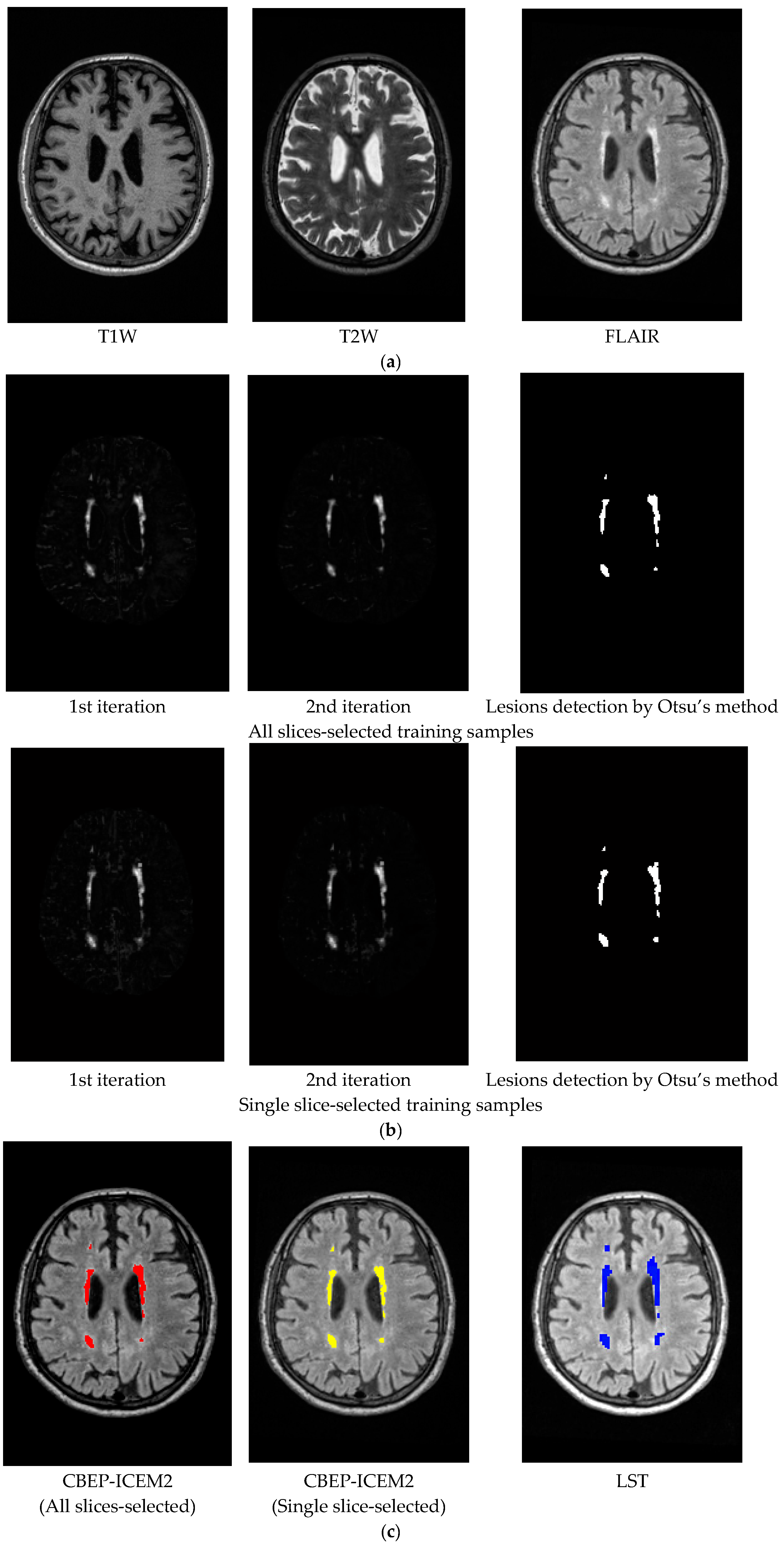
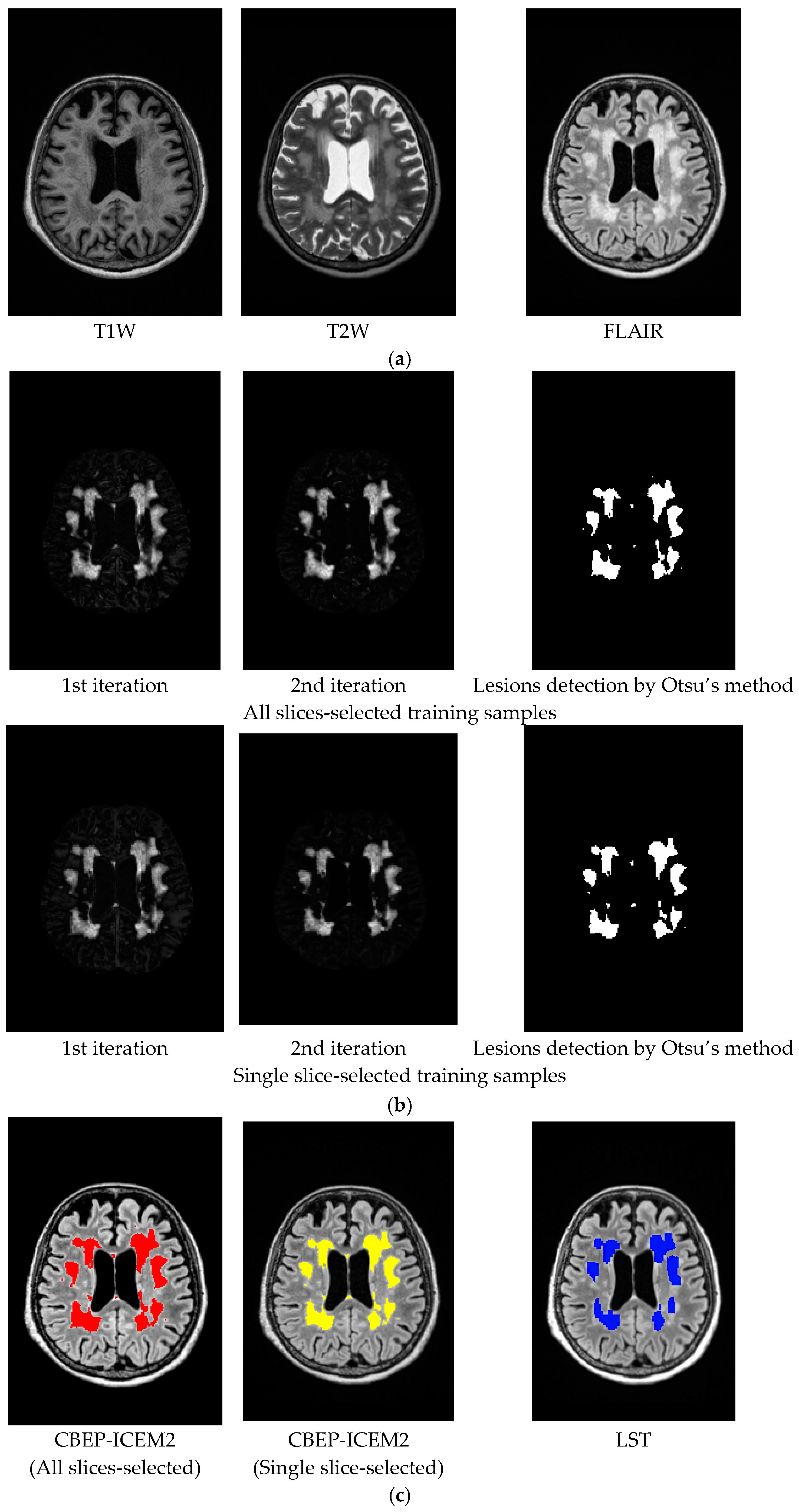
3.2. Real Image Experiments

Real MRI brain images were acquired at the Taichung Veterans General Hospital (TCVGH) by Siemens Magnetom Aera 1.5 Tesla (Erlangen, Germany) MR scanner with a 16-channel phase-array head coil. MR imaging protocol included T1W with 3D MPRAGE, T2W and FLAIR. Since T1W, T2W and FLAIR images used for experiments were collected by 3D high resolution sequences with each voxel of size, 1 × 1 × 1 mm3, the interpolation artifacts and partial volume do not have much effect on imaging. However, as a part of trade-off, this also requires additional 2 min for image acquisition. Other imaging parameters used for data acquisition were voxel size of 1 × 1 × 1 mm3, matrix size = 256 × 256 × 176, NEX = 1. According to a clinical visual inspection criterion [27], the WMH lesions can be graded by Fazekas with three grades of Fazekas shown in Figure 11 for illustration.
A total of 111 cases were collected and all the participants have been well-informed and signed their consents. In addition, the study conducted in this paper was approved by the Ethics Committee of Clinical Research, Taichung Veterans General Hospital (IRB number: CE16138A). Among all the 111 cases there are 58 cases of Fazekas grade 1, 44 cases of Fazekas grade 2 and 9 cases of Fazekas grade 3. Thus, in this study, we selected 10 cases from Fazekas grade 1, 11 cases from Fazekas grade 2, and 9 cases from Fazekas grade 3.
As demonstrated by synthetic image experiments, CBEP-ICEM2 was shown to be a better WMH detection technique. Thus, CBEP-ICEM 2 was used in real image experiments. Table 4 tabulates the values of parameters used by CBEP-ICEM2 where two sets of training samples selected by all slices and the single 90th slice were selected to calculate the desired target signature d to implement NBE-ICEM.
Figure 12, Figure 13 and Figure 14 show the WMH lesion detection results produced by CBEP-ICEM2 and LST for three Fazekas grades, respectively, where Figure 12a, Figure 13a and Figure 14a are original T1W, T2W and FLAIR MR images; Figure 12b, Figure 13b and Figure 14b are iterative WMH lesion detection images by CBEP-ICEM2 along with final WMH lesion detection by Otsu’s method; and Figure 12c, Figure 13c and Figure 14c show comparisons between lesion detections by CBEP-ICEM2 and LST.
As demonstrated in Figure 12, Figure 13 and Figure 14, our proposed NBE-ICEM using two sets of training samples performed very similarly and also better than LST according to clinical visual evaluation criterion, Fazekas grades [27].

4. Discussion

This paper is believed to be the first work ever reported in the literature to attempt to use a hyperspectral subpixel detection, NBE-ICEM, to detect WMHs on MRI. As demonstrated in Table 2 and Table 3 and Figure 5, Figure 6, Figure 7, Figure 8, Figure 9 and Figure 10 and Figure 12, Figure 13 and Figure 14 the synthetic and real image experiments confirm significant improvements using NBE-ICEM over the LST method in WMH detection.
In comparison between CBEP-CEM1 and CBEP-CEM2, we found from Table 2 and Table 3 in the synthetic image experiments that, when the noise level is low (0%, 1%, 3%), CBEP-ICEM1 using a smaller Gaussian window performed better than CBEP-ICEM2 using a larger Gaussian window. However, when the noise level is high (5%, 7%, 9%), the conclusion is reversed, i.e., CBEP-ICEM2 performed better than CBEP-ICEM1. It is also interesting to note that CBEP-ICEM1 performed very poorly when noise level reached 7% and above and even worse than LST. Table 2 and Table 3 also shown that it was noise not INU that had an impact on lesion detection. On the other hand, CBEP-ICEM2 generally performed well regardless of noise level if DSI value was set to at least or above 0.8 compared to LST whose DSI values did not go beyond 0.8. The synthetic image experiments suggested that CBEP-ICEM2 was a better technique due to its robustness to noise level and ability in WMH detection.
In addition, based on the results of real image experiments from Figure 12, Figure 13 and Figure 14, there are three interesting findings. Firstly, the number of iterations carried out by CBEP-ICEM is always two for all three Fazekas grades. Secondly, in Figure 12c, CBEP-ICEM2 and LST performed similarly but quite different in Figure 13c and Figure 14c, where the areas of lesions detected by LST were much smaller than CBEP-ICEM2. Thirdly, the iterative images produced in Figure 12b, Figure 13b and Figure 14b by CBEP-ICEM2 showed that including spatial information captured by Gaussian-filtered CEM detection images did improve lesion detection, particularly edge and boundary pixels.
This paper makes several main contributions to WMH lesions detection in MR brain images. First, it develops NBE to resolve two issues arising in WMH detection, insufficient spectral dimensionality and linear non-separability problem. NBE plays a similar role that kernels play in pattern classification such as support vector machine (SVM). Second, it introduces Gaussian filters to be included in CEM to expand capability of CEM in capturing spatial information surrounding CEM-detected WMH lesions. Third, the real-valued CEM-detection abundance fractional maps provide soft decisions for visual inspection. Fourth, Otsu’s method is incorporated in ICEM to produce thresholded binary maps as hard decisions that show WMH lesions detection. This resolves the main issue encountered in LST. Fifth, the feedbacks of Gaussian filtered CEM detection abundance fractional maps allow CEM to perform better detection in WMH lesions when spatial information of lesions is crucial, specifically, their boundaries. Finally, an automatic stopping rule is particularly designed to determine how much spatial information is needed for CEM to perform its best in detection of WMH lesions.

5. Conclusions

In conclusion, this paper develops a novel approach, called NBE-ICEM, for WMH lesions detection in MR brain images. It is derived from a hyperspectral imaging-based subpixel target detection method (CEM), but is rather different from CEM in two aspects. One is an introduction of NBE into CEM, which expands the original MR images by including nonlinearly correlated band images generated by NBE to make a multispectral MR image into a hyperspectral MR image since CEM is a hyperspectral imaging technique. The other is the development of an iterative version of CEM, ICEM, which can feed back spatial information captured by Gaussian filters in an iterative manner. More specifically, it applies a Gaussian filter to CEM-detection maps to produce Gaussian-filtered CEM-detected abundance fractional maps that can be further fed back iteratively to form a new set of MR image cubes which will be used a new data set to be re-processed by CEM to improve WMH lesions detection performance. ICEM can be considered as a joint spectral–spatial filter. The more iterations carried out by ICEM, the more spatial information captured. The work on NBE-ICEM presents a potential and promising technique for WMH lesions detection. It is our belief that there would be new applications of NBE-ICEM to MRI yet to explore in the future, specifically, partial volume estimation for specific tissues of interest.

Acknowledgments

The work of this paper was supported by grants from Taichung Veterans General Hospital (TCVGH-1047315C, and TCVGH-1057315C), and grants from Ministry of Science and Technology (MOST 104-2221-E-075A-002, and MOST-105-2221-E-075A-001). The work of L. Wang is supported by the Fundamental Research Funds for Central Universities under Grant JB150508 and the 111 Project (B17035). The works of Y. Wang and M. Song are supported by Fundamental Research Funds for Central Universities (3132016028 and 3132016331) and National Nature Science Foundation of China (61601077 and 61301228), respectively. The work of C.-I Chang is supported by the Fundamental Research Funds for Central Universities under Grant 3132016331.

Author Contributions

H.-M.C., J.-W.C., and C.-C.C.C. conceived and designed the experiments; L.W., C.Y., and Y.W. performed the experiments; H.C.W., M.S., and B.X. analyzed the data; C.-I.C., H.-M.C., J.-W.C., and C.-C.C.C. contributed reagents/materials/analysis tools; C.-I C. wrote the paper.

Conflicts of Interest

All authors have declared no conflict of interest.

References

  1. Callisaya, M.L.; Beare, R.; Phan, T.; Blizzard, L.; Thrift, A.G.; Chen, J.; Srikanth, V.K. Progression of White Matter Hyperintensities of Presumed Vascular Origin Increases the Risk of Falls in Older People. J. Gerontol. A Biol. Sci. Med. Sci. 2015, 70, 360–366. [Google Scholar] [CrossRef] [PubMed]
  2. Hachinski, V.C.; Potter, P.; Merskey, H. Leuko-araiosis: an ancient term for a new problem. Can. J. Neurol. Sci. J. Can. Sci. Neurol. 1986, 13, 533–534. [Google Scholar] [CrossRef]
  3. Boutet, C.; Rouffiange-Leclair, L.; Schneider, F.; Camdessanché, J.-P.; Antoine, J.-C.; Barral, F.-G. Visual Assessment of Age-Related White Matter Hyperintensities Using FLAIR Images at 3 T: Inter- and Intra-Rater Agreement. Neurodegener. Dis. 2015. [Google Scholar] [CrossRef] [PubMed]
  4. Valverde, S.; Oliver, A.; Roura, E.; González-Villà, S.; Pareto, D.; Vilanova, J.C.; Ramió-Torrentà, L.; Rovira, À.; Lladó, X. Automated tissue segmentation of MR brain images in the presence of white matter lesions. Med. Image Anal. 2017, 35, 446–457. [Google Scholar] [CrossRef] [PubMed]
  5. Roura, E.; Oliver, A.; Cabezas, M.; Valverde, S.; Pareto, D.; Vilanova, J.C.; Ramió-Torrentà, L.; Rovira, À.; Lladó, X. A toolbox for multiple sclerosis lesion segmentation. Neuroradiology 2015, 57, 1031–1043. [Google Scholar] [CrossRef] [PubMed]
  6. Samaille, T.; Fillon, L.; Cuingnet, R.; Jouvent, E.; Chabriat, H.; Dormont, D.; Colliot, O.; Chupin, M. Contrast-Based Fully Automatic Segmentation of White Matter Hyperintensities: Method and Validation. PLoS ONE 2012, 7. [Google Scholar] [CrossRef] [PubMed]
  7. Gibson, E.; Gao, F.; Black, S.E.; Lobaugh, N.J. Automatic segmentation of white matter hyperintensities in the elderly using FLAIR images at 3T. J. Magn. Reson. Imaging 2010, 31, 1311–1322. [Google Scholar] [CrossRef] [PubMed]
  8. Vannier, M.W.; Butterfield, R.L.; Jordan, D.; Murphy, W.A.; Levitt, R.G.; Gado, M. Multispectral analysis of magnetic resonance images. Radiology 1985, 154, 221–224. [Google Scholar] [CrossRef] [PubMed]
  9. Chang, C.-I. Hyperspectral Imaging: Techniques for Spectral Detection and Classification; Springer: New York, NY, USA, 2003; ISBN 978-0-306-47483-5. [Google Scholar]
  10. Nakai, T.; Muraki, S.; Bagarinao, E.; Miki, Y.; Takehara, Y.; Matsuo, K.; Kato, C.; Sakahara, H.; Isoda, H. Application of independent component analysis to magnetic resonance imaging for enhancing the contrast of gray and white matter. NeuroImage 2004, 21, 251–260. [Google Scholar] [CrossRef] [PubMed]
  11. Ouyang, Y.-C.; Chen, H.-M.; Chai, J.-W.; Chen, C.-C.; Chen, C.C.-C.; Poon, S.-K.; Yang, C.-W.; Lee, S.-K. Independent Component Analysis for Magnetic Resonance Image Analysis. EURASIP J. Adv. Signal Process. 2008, 2008. [Google Scholar] [CrossRef]
  12. Ouyang, Y.-C.; Chen, H.-M.; Chai, J.-W.; Chen, C.C.-C.; Poon, S.-K.; Yang, C.-W.; Lee, S.-K.; Chang, C.-I. Band Expansion-Based Over-Complete Independent Component Analysis for Multispectral Processing of Magnetic Resonance Images. IEEE Trans. Biomed. Eng. 2008, 55, 1666–1677. [Google Scholar] [CrossRef] [PubMed]
  13. Chai, J.-W.; Chen, C.C.-C.; Chiang, C.-M.; Ho, Y.-J.; Chen, H.-M.; Ouyang, Y.-C.; Yang, C.-W.; Lee, S.-K.; Chang, C.-I. Quantitative analysis in clinical applications of brain MRI using independent component analysis coupled with support vector machine. J. Magn. Reson. Imaging 2010, 32, 24–34. [Google Scholar] [CrossRef] [PubMed]
  14. Chai, J.-W.; Chen, C.C.; Wu, Y.-Y.; Chen, H.-C.; Tsai, Y.-H.; Chen, H.-M.; Lan, T.-H.; Ouyang, Y.-C.; Lee, S.-K. Robust Volume Assessment of Brain Tissues for 3-Dimensional Fourier Transformation MRI via a Novel Multispectral Technique. PLOS ONE 2015, 10. [Google Scholar] [CrossRef] [PubMed]
  15. Chiou, Y.-J.; Chen, C.C.-C.; Chen, S.-Y.; Chen, H.-M.; Chai, J.-W.; Ouyang, Y.-C.; Su, W.-C.; Yang, C.-W.; Lee, S.-K.; Chang, C.-I. Magnetic resonance brain tissue classification and volume calculation. J. Chin. Inst. Eng. 2015, 38, 1055–1066. [Google Scholar] [CrossRef]
  16. Ren, H.; Chang, C.-I. A generalized orthogonal subspace projection approach to unsupervised multispectral image classification. IEEE Trans. Geosci. Remote Sens. 2000, 38, 2515–2528. [Google Scholar]
  17. Harsanyi, J.C. Detection and Classification of Subpixel Spectral Signatures in Hyperspectral Image Sequences; Department of Electrical Engineering, University of Maryland, Baltimore County: Baltimore, MD, USA, 1993. [Google Scholar]
  18. Farrand, W.H.; Harsanyi, J.C. Mapping the distribution of mine tailings in the Coeur d’Alene River Valley, Idaho, through the use of a constrained energy minimization technique. Remote Sens. Environ. 1997, 59, 64–76. [Google Scholar] [CrossRef]
  19. Chang, C.-I. Target signature-constrained mixed pixel classification for hyperspectral imagery. IEEE Trans. Geosci. Remote Sens. 2002, 40, 1065–1081. [Google Scholar] [CrossRef]
  20. Xue, B.; Wang, L.; Li, H.-C.; Chen, H.M.; Chang, C.-I. Lesion Detection in Magnetic Resonance Brain Images by Hyperspectral Imaging Algorithms. In Proceedings Volume 9874, Remotely Sensed Data Compression, Communications, and Processing XII; International Society for Optics and Photonics: Baltimore, MD, USA, 2016; Vol. 9874, p. 98740M. [Google Scholar]
  21. Otsu, N. A threshold selection method from gray-level histgram. IEEE Trans. Syst. Man Cybern. 1979, 9, 62–66. [Google Scholar] [CrossRef]
  22. Dice, L.R. Measures of the amount of ecologic association between species. Ecology 1945, 26, 297–302. [Google Scholar] [CrossRef]
  23. Kang, X.; Li, S.; Benediktsson, J.A. Spectral-Spatial Hyperspectral Image Classification with Edge-Preserving Filtering. IEEE Trans. Geosci. Remote Sens. 2014, 52, 2666–2677. [Google Scholar] [CrossRef]
  24. BrainWeb: Simulated Brain Database. Available online: http://www.bic.mni.mcgill.ca/brainweb/ (accessed on 15 November 2017).
  25. LST: A Lesion Segmentation Tool for SPM. Available online: http://www.statistical-modelling.de/lst.html (accessed on 15 November 2017).
  26. Schmidt, P.; Gaser, C.; Arsic, M.; Buck, D.; Förschler, A.; Berthele, A.; Hoshi, M.; Ilg, R.; Schmid, V.J.; Zimmer, C.; et al. An automated tool for detection of FLAIR-hyperintense white-matter lesions in Multiple Sclerosis. NeuroImage 2012, 59, 3774–3783. [Google Scholar] [CrossRef] [PubMed]
  27. Fazekas, F.; Chawluk, J.B.; Alavi, A.; Hurtig, H.I.; Zimmerman, R.A. MR signal abnormalities at 1.5 T in Alzheimer’s dementia and normal aging. Am. J. Roentgenol. 1987, 149, 351–356. [Google Scholar] [CrossRef] [PubMed]
Figure 1. A diagram of the kth iteration carried out by hyperspectral image classification implementing ICEM on Ω NBE ( k )
Remotesensing 09 01174 g001
Figure 2. A flow chart of the stopping rule used for NBE-ICEM.
Remotesensing 09 01174 g002
Figure 3. Graphic implementation of NBE-ICEM in Figure 1.
Remotesensing 09 01174 g003
Figure 4. Three MR images containing MS lesions acquired by T1W, T2W and PD with 0% noise and 0% INU. (a) T1W; (b) T2W; (c) PD; (d) ground truth (lesions)
Remotesensing 09 01174 g004
Figure 5. Lesion detection of Slice 97 with 0% noise and 0% INU by CBEP-ICEM1 and CBEP-ICEM2. (a) CBEP-ICEM1; (b) CBEP-ICEM2; (c) Lesion detection LST.
Remotesensing 09 01174 g005
Figure 6. Lesion detection of Slice 97 with 1% noise and 0% INU by CBEP-ICEM1 and CBEP-ICEM2. (a) Original 97th slice of MS MR brain images with 1% noise and 0% INU; (b) CBEP-ICEM1; (c) CBEP-ICEM2; (d) Lesion detection LST.
Remotesensing 09 01174 g006aRemotesensing 09 01174 g006b
Figure 7. Lesion detection of Slice 97 with 3% noise and 0% INU by CBEP-ICEM1 and CBEP-ICEM2. (a) Original 97th slice of MS MR brain images with 3% noise and 0% INU; (b) CBEP-ICEM1; (c) CBEP-ICEM2; (d) Lesion detection LST.
Remotesensing 09 01174 g007aRemotesensing 09 01174 g007b
Figure 8. Lesion detection of Slice 97 with 5% noise and 0% INU by CBEP-ICEM1 and CBEP-ICEM2. (a) Original 97th slice of MS MR brain images with 5% noise and 0% INU; (b) CBEP-ICEM1; (c) CBEP-ICEM2; (d) Lesion detection LST.
Remotesensing 09 01174 g008aRemotesensing 09 01174 g008bRemotesensing 09 01174 g008c
Figure 9. Lesion detection of Slice 97 with 7% noise and 0% INU by CBEP-ICEM1 and CBEP-ICEM2. (a) Original 97th slice of MS MR brain images with 7% noise and 0% INU; (b) CBEP-ICEM1; (c) CBEP-ICEM2; (d) Lesion detection LST.
Remotesensing 09 01174 g009aRemotesensing 09 01174 g009b
Figure 10. Lesion detection of Slice 97 with 9% noise and 0% INU by CBEP-ICEM1 and CBEP-ICEM2. (a) Original 97th slice of MS MR brain images with 9% noise and 0% INU; (b) CBEP-ICEM1; (c) CBEP-ICEM2; (d) Lesion detection LST.
Remotesensing 09 01174 g010aRemotesensing 09 01174 g010b
Figure 11. Lesion categorized by three grades of Fazekas shown in FLAIR images. (a) Fazekas grade 1; (b) Fazekas grade 2; (c) Fazekas grade 3
Remotesensing 09 01174 g011
Figure 12. Lesion detection of Fazekas grade 1 by CBEP-ICEM2 and LST (a) Original MR images (T1W, T2W, FLAIR) with lesions of Fazekas grade 1; (b) CBEP-ICEM2-detected lesion of Fazekas grade 1; (c) Comparison between lesion detections by CBEP-ICEM2 and LST.
Remotesensing 09 01174 g012
Figure 13. Lesion detection of Fazekas grade 2 By CBEP-ICEM2 and LST. (a) Original MR images (T1W, T2W, FLAIR) with lesions of Fazekas grade 2; (b) Lesion detection by CBEP-ICEM2; (c) Comparison between lesion detections by CBEP-ICEM2 and LST.
Remotesensing 09 01174 g013
Figure 14. Lesion detection of Fazekas grade 3 By CBEP-ICEM2 and LST. (a) Original MR images (T1W, T2W, FLAIR) with lesions of Fazekas grade 3; (b) Lesion detection by CBEP-ICEM2; (c) Comparison between lesion detections by CBEP-ICEM2 and LST.
Remotesensing 09 01174 g014
Table 1. Specifications of parameters used by NBE-ICEM for BrainWeb images.
Band imagesT1W, T2W, PD (3 bands)
Correlation Band Expansion Process (CBEP)3rd order correlated band images
dfound by all slices-selected or single slice-selected training samples
Gaussian window size 3 × 3 ( 5 × 5 )
σ used in Gaussian filter0.1 with window size 3 × 3 (0.5 with window size 5 × 5 )
Thresholding methodOtsu’s method
error threshold (DSI)0.80
Table 2. Averaged DSI values of lesions detection by CBEP-ICEM1, CBEP-ICEM2 and LST over MR image slices 91–113.
MethodsCBEP-ICEM1CBEP-ICEM2LST
Noise/INU Level
n0/rf00.8650.8080.739
n1/rf00.8860.8640.749
n3/rf00.8930.8630.750
n5/rf00.8060.8390.731
n7/rf00.6520.8220.693
n9/rf00.5790.8010.714
n0/rf200.8610.8290.733
n1/rf200.8670.8340.753
n3/rf200.8810.8270.746
n5/rf200.8140.8310.732
n7/rf200.7140.8250.694
n9/rf200.5400.8060.655
Table 3. Averaged DSI values of lesions detection by CBEP-ICEM1, CBEP-ICEM2 and LST over MR image slices 91–113 using slice 102 to select training samples.
MethodsCBEP-ICEM1CBEP-ICEM2LST
Noise/INU Level
n0/rf00.7980.7840.739
n1/rf00.8480.8470.749
n3/rf00.8710.8580.750
n5/rf00.7760.8360.731
n7/rf00.6250.8160.693
n9/rf00.3890.7780.714
n0/rf200.8440.8340.733
n1/rf200.8590.8370.753
n3/rf200.8540.8140.746
n5/rf200.8110.8190.732
n7/rf200.7100.8040.694
n9/rf200.5490.7990.655
Table 4. Parameters used by CBEP-ICEM2.
BandT1W, T2W, FLAIR (3 bands)
CBEP3rd order correlated band images
dfound by all slices-selected or single slice-selected training samples
Fazekas grade123
Gaussian window size5 × 5
σ used in Gaussian filter0.5 with window size 5 × 5
Thresholding methodOtsu’s method
stopping threshold (DSI)0.80

