Technical Note

Measurement of Precipitation in the Alps Using Dual-Polarization C-Band Ground-Based Radars, the GPM Spaceborne Ku-Band Radar, and Rain Gauges

1
MeteoSwiss, via ai Monti 146, CH-6605 Locarno-Monti, Switzerland
2
Environmental Remote Sensing Lab, EPFL, CH-1015 Lausanne, Switzerland
3
Institute of Applied Physics, University of Bern, CH-3012 Bern, Switzerland
*
Author to whom correspondence should be addressed.
Remote Sens. 2017, 9(11), 1147; https://doi.org/10.3390/rs9111147
Submission received: 31 July 2017 / Revised: 26 October 2017 / Accepted: 2 November 2017 / Published: 8 November 2017

Abstract

:
The complex problem of quantitative precipitation estimation in the Alpine region is tackled from four different points of view: (1) the modern MeteoSwiss network of automatic telemetered rain gauges (GAUGE); (2) the recently upgraded MeteoSwiss dual-polarization Doppler, ground-based weather radar network (RADAR); (3) a real-time merging of GAUGE and RADAR, implemented at MeteoSwiss, in which a technique based on co-kriging with external drift (CombiPrecip) is used; (4) spaceborne observations, acquired by the dual-wavelength precipitation radar on board the Global Precipitation Measuring (GPM) core satellite. There are obviously large differences in these sampling modes, which we have tried to minimize by integrating synchronous observations taken during the first 2 years of the GPM mission. The data comprises 327 “wet” overpasses of Switzerland, taken after the launch of GPM in February 2014. By comparing the GPM radar estimates with the MeteoSwiss products, a similar performance was found in terms of bias. On average (whole country, all days and seasons, both solid and liquid phases), underestimation is as large as −3.0 (−3.4) dB with respect to RADAR (GAUGE). GPM is not suitable for assessing what product is the best in terms of average precipitation over the Alps. GPM can nevertheless be used to evaluate the dispersion of the error around the mean, which is a measure of the geographical distribution of the error inside the country. Using 221 rain-gauge sites, the result is clear both in terms of correlation and in terms of scatter (a robust, weighted measure of the dispersion of the multiplicative error around the mean). The best agreement was observed between GPM and CombiPrecip, and, next, between GPM and RADAR, whereas a larger disagreement was found between GPM and GAUGE. Hence, GPM confirms that, for precipitation mapping in the Alpine region, the best results are obtained by combining ground-based radar with rain-gauge measurements using a geostatistical approach. The GPM mission is adding significant new coverage to mountainous areas, especially in poorly instrumented parts of the world and at latitudes not previously covered by the Tropical Rainfall Measuring Mission (TRMM). According to this study, one could expect an underestimation of the precipitation product by the dual-frequency precipitation radar (DPR) also in other mountainous areas of the world.

Graphical Abstract

1. Introduction

With the introduction of a precipitation radar on board the Tropical Rainfall Measuring Mission (TRMM) satellite, meteorological radar applications could be expanded to the oceans and lands between ±35° latitude on Earth. The Global Precipitation Measurement (GPM) mission Core Observatory satellite, launched on 27 February 2014 [1], has extended the TRMM coverage to ±65° latitude, hence including the Alps. Because of the roughly 5 km diameter footprint of the GPM dual-frequency precipitation radar (DPR), clutter contamination will typically limit GPM measurements to areas above the mountains, except where very broad valleys are present. The DPR adds significant new coverage to orographically complex areas, especially in poorly instrumented regions of the world.
Precipitation in orographically complex regions like the Alps is inherently complex because of the interactions between the mountainous terrain and the atmosphere. The resultant effects have been the subject of extensive research (e.g., [2]). Additionally, the higher altitudes (and hence lower temperatures) mean that a large proportion of precipitation falls in solid phase, resulting in significant amounts of water being stored in the Alps as snow. This makes the mountains a vital water source in many parts of the world. Better knowledge of precipitation fields in the Alps is necessary in weather, nowcasting, and climate research, and more accurate precipitation measurements, especially in orographically complex catchments, are essential to develop reliable warnings. However, the same complex orography and colder temperatures that make the Alpine environment an important water reservoir in Europe, also make the measurement of precipitation challenging not only for spaceborne radars, but also for ground-based weather radars. The rough and complex orography together with cold and windy conditions make the installation of large radar antennas difficult [3]; the terrain may cause partial or almost total shielding of the radar beam, restricting measurements to high altitudes (e.g., [4,5,6]). Unfortunately, the well-known sources of error that affect radar estimations (e.g., [7,8,9,10]) become particularly severe in mountainous terrain (e.g., [11,12]).
Rain gauges are usually considered to provide accurate “point” measurements. In this context, “point” means a gauge cross section that is usually 200 cm2 (and a sampling volume of the order of ~60 m3 every 10 min, assuming, for instance, an average terminal fall velocity of 4 m/s). Consequently, it is well known that gauge observations represent local effects and not areal quantities. For hydrological applications, areal precipitation estimates are required, and, therefore, their main drawback is undersampling [13], i.e., there will not be enough observations to describe the variability of the field. Because of the spatial variability of rainfall (especially during intense, convective events), it is obvious that point measurements would undersample the precipitation fields, even though the measurements themselves were correct. Radar measurements can add the desired information on the areal distribution of precipitation. There are enormous differences between remotely sensed radar observations and in situ point measurements by the rain gauges. On the one hand, the small-scale variability of precipitation is such that even three decades ago Austin [14] wrote that “the spatial variability of rainfall is so pronounced that a single gauge often does not sample representatively over any area, even as small as 4 km2”. On the other hand, spatial smoothing by the main Gaussian lobe of the radar antenna radiation pattern, as well as post-detection integration over many pulses reduce the variability of the distribution of precipitation rate in space. Even in the liquid phase, when radar data are compared with “instantaneous” point rainfall rate, a random error and a bias are introduced by the smoothing [15]. This explains some of the difficulties in the use of radars for quantitative precipitation estimations. When gauge data are also smoothed in time, the random error and the bias are reduced.
Various deterministic or statistical methods for radar–gauge merging have been proposed. Many applications of these tools have appeared in the literature, all of which provide valuable contributions to the common knowledge regarding the problem at hand (e.g., [16,17,18,19,20,21,22]). In Switzerland, the merging of radar and rain gauge measurements is based on spatio-temporal kriging with external drift [22]; it was implemented at MeteoSwiss five years ago and it has been run operationally since then. This product is called CombiPrecip.
To summarize, in the Swiss Alps there are currently three different ground-measured precipitation products available: (1) a product based on a network of automatic telemetered rain gauges (GAUGE); (2) a product based on a state-of-the art, C-band, dual-polarization Doppler, ground-based weather radar network (RADAR); and (3) a product consisting in a real-time merging of observations from these two networks, implemented and operational at MeteoSwiss (CombiPrecip). In this paper, we compare these products with another product based on the GPM spaceborne radar, which should provide the best space-based instantanous rainfall rate estimations.
Several authors (e.g., [13,15,23]) illustrate the problems of the two types of instruments (radars and gauges) concerning the large scatter of “short time-scale” values for a given location, which are caused by the huge differences in the sampling modes. In many cases, and certainly for our evaluation purposes, it is wise to integrate the measurements over time. An integration over long times also reduces the differences in the retrieved estimates between the spaceborne and the ground-based radars. Although these two sensors certainly have more similarities than a radar and a rain gauge, there are nevertheless enormous differences between the two. In this regard, mention can be made of the different operating frequencies, sampling volumes, geometrical viewing angles, attenuation, sensitivity, and temporal resolution (see Section 2.1 and Section 2.2).
Consequently, in this short note aimed at evaluating the performance of three Swiss precipitation products (RADAR, GAUGE, and their combination, i.e., CombiPrecip) in comparison with GPM, a 2 year integration period is used to minimize the large differences in the sampling modes between the various instruments. During this period, the same number of rain gauges (221) and ground-based radars (four) were used. Obviously, only RADAR, GAUGE, and CombiPrecip observations that were closest in time to GPM overpasses are used to derive the total precipitation amounts in every 25 km2 reference pixel (see Section 2.1 and Section 2.2.3 for more details). The GPM precipitation product underestimates, on average, the precipitation in Switzerland by a factor of 2 (−3 dB) with respect to RADAR, and by a factor of −3.4 dB with respect to GAUGE. However, GPM estimates are used to independently evaluate the three Swiss products in terms of dispersion of the error around the mean (as well as of correlation among the various precipitation products), rather than in terms of exact average amount of 2 year precipitation over the country (mean error). To the best of the authors’ knowledge, this is the first attempt to compare in complex terrain four precipitation products that use three very different types of sensors. Using GPM as a reference, the best precipitation product results to be the combination, through a geostatistical approach, of ground-based radar and rain-gauge measurements.
This fact is thoroughly described in Section 3, which presents the results. The findings and their implications are discussed Section 4, which presents also future research directions. Section 2 gives an overview of the instruments and precipitation products used, and describes the study area and methods. A conclusion is given in Section 5.

2. Materials and Methods

In this study an evaluation of three MeteoSwiss sources of precipitation data (conventional in situ measurements, remotely sensed observations, and a geostatistical merging of these two) is conducted using the GPM-DPR level 2 estimated surface precipitation products as a reference. As stated in the introduction, we have tried to minimize the huge differences in the sampling modes by integrating over time several hundreds of synchronous observations (to be precise, 528 satellite overpasses) from 9 March 2014 (when the first GPM precipitation data became available over Switzerland) to 29 February 2016.

2.1. Global Precipitation Measurement Spaceborne Radar (GPM-DPR) Data

The GPM-DPR consists essentially of two radars operated in tandem and with similar antenna radiation pattern. The Ku-band (13.54 GHz) radar is very similar to that found on TRMM and scans a swath that is approximately 245 km wide across the satellite track, measuring some 49 footprints of approximately 5 km in diameter and with 250 m vertical resolution at the nadir. Figure 1 in [24] shows the shape of such footprints as well as their coarsening in terms of vertical resolution with increasing distance from the nadir (the vertical resolution degrades from 250 m to ~1700 m at 17° from the nadir). The Ka-band (35 GHz) radar matches the scan of the Ku-band radar across the central 125 km of its swath, allowing for the application of dual-frequency algorithms (obviously reducing the coverage to the central swath). Hence, on the one hand, the use of the dual-frequency algorithm and observations would limit the number of available overpasses to 393, as can be seen in [25] (Table 2, p. 1252), whereas, on the other hand, the use of the second frequency slightly improves the GPM precipitation estimates in the Swiss Alps and plateau, as can be seen in [25] Table A1 (p. 1266) and A2 (p. 1267). Consequently, in this study we opted to maximize the number of overpasses and synchronous observations (528, see Table 2 in [25]), and this implies that the 35 GHz measurements are not considered.
The GPM data used in this study are the Ku-band level 2 data, version V04A and V05A. As for TRMM, the GPM level 2 data include many variables, but the key variable evaluated in this work is the estimated surface precipitation rate (“precipRateESurface”), although, in practice, there is little difference between this variable and the classical TRMM variable (“precipRateNearSurface”). The GPM level 2-DPR product is unlikely to be as broadly used as ground-based measurements or level 3 satellite precipitation accumulation products [26,27,28,29,30]. However, it is vitally important to the ground validation study using dense radar and gauge network (like the present study) and to the generation of the level-3 products.
The location and vertical resolution of GPM level 2 cells are different from one overpass to another. Using a nearest-neighbor approach, each estimated surface precipitation rate was simply assigned to a GPM-like 25 km2 reference pixel (see, for instance, Figures S2–S4) based on a Cartesian grid that is coincident with the Swiss national coordinate system (CH1903). In brief, the Swiss coordinates result from a conformal mapping from the Bessel reference ellipsoid onto a longitudinal cylinder, tangential in Bern, having the cross section correspondent to the great circle of the approximating sphere perpendicular to the Earth meridian passing across Bern. The tangential point has coordinates (600, 200; km).

2.2. The Latest MeteoSwiss Dual-Polarization Weather Radar (RADAR) Network Data

In 2011, MeteoSwiss started the renewal of its weather radar network: it now consists of five identical, dual-polarization, Doppler, C-band (5.5 GHz) radars [3]. Antenna-mounted, fully-digital receivers have been introduced into the design and implementation of the current systems; each system is equipped with two orthogonal receiving channels, which are able to measure vertical and horizontal linear polarizations. Three of these radars are located near the political borders of Switzerland (to control fronts and detect perturbations in the largest possible range) and close to highly populated areas and large airports; these locations are the same as in the previous network. Two additional radars have been installed, by necessity, at high altitudes (3000 m), to improve the coverage in the inner parts of the Alps. The radar locations (latitude, longitude, altitude) are listed in [25] (Table 1, p. 1250) and shown in [25] (Figure 1, p. 1250). During the period covered by this study, the three radars were installed and operational all time long; the high altitude radars in Valais (above Crans-Montana) and above Davos (close to Austria) entered the mosaic in May 2014, and at the end of 2015, respectively.
Radar hardware monitoring is run continuously: more than 350 parameters are monitored and submitted from each radar site to the central server after completion of every single sweep, that is 20 times in 5 min. The parameters are automatically checked for anomalies and archived for diagnostic analyses. Daily monitoring of the radar receiver and pointing accuracy of the antenna radiation main lobe are also implemented [31] following the Dutch-Finnish [32,33] operational monitoring approach. A guiding principle for a comprehensive monitoring is to combine as many independent sources of information as possible. These include various types of weather echoes, ground clutter signals, signals from the sun, signals transmitted by the radar and measured by an external receiver, signals received by an external transponder and transmitted back to the radar with a shift in time, intensity, frequency and polarization, signals reflected by nearby towers, and test signals inserted at various locations by laboratory test equipment during preventive maintenance.

2.2.1. Relative and Absolute Calibration of the Ground-Based Radars

In order to guarantee system stability and reproducibility, instrumental calibration of the radar using an internal microwave equipment must be implemented. In our approach at MeteoSwiss, internal calibration is continuous, automatic and done independently for both polarization channels. A reference power from a stable source is injected, and that value (± a given uncertainty) is read by the receiver. This concept for relative calibration does not require any signal from external active or passive sources. It has to compensate for variations of the radar equipment, and thus guarantees stable conditions for precipitation measurement. It is of particular importance after any maintenance, especially a corrective maintenance with component replacement. Hence, the parameter of relative calibration defines our ability to reproduce in the future the values we measure today. For the MeteoSwiss radars, relative calibration is performed continuously and automatically using a noise source [34] and an integrated test signal generator, as well as offline during preventive maintenance. The noise source signal is inserted every 2.5 min in both polarization channels of the receive path, both before the T/R limiter and at the entrance of the first stage of the low noise amplifiers.
Absolute calibration of the whole radar refers to the electrical–electromagnetic tuning of the system versus some known reference targets (e.g., a metal sphere or other reflectors with known radar cross sections) at various ranges. This requires detailed knowledge of the whole system, including losses of the receiver and transmitter chains, antenna gain, random losses, noise factor, matched filter losses, and atmospheric attenuation. Apart from few experiments during the site acceptance tests using the armasuisse Time Stamp Amplitude equipment (TSAMP) and radar target simulator (RTS) [35], absolute calibration of both transmit and receive chains is not envisaged in the MeteoSwiss current generation network. Nevertheless, absolute calibration accuracy of the receive chains (vertical and horizontal polarization) is checked on demand, typically a few times per year, using the methodology presented in [36].

2.2.2. Adjustment of Radar-Derived Mean (Precipitation) Field Bias Using Selected Rain Gauges

Adjustment refers to the a posteriori, physical and meteorological tuning of radar estimates versus a very large set of representative reference measurements of the variable of interest. For precipitation estimation, reference measurements come from conventional in situ point measurements by rain gauges, which, by integration in time and space, should be comparable to the large radar sampling volume. While relative calibration should be carried out continuously and automatically, the adjustment of the mean precipitation fields is a long-term task, which is performed offline (using very long observation periods) and applied as rarely as possible. For instance, for the previous MeteoSwiss weather radar network, no mean field bias (MBF) adjustment was necessary to any of the three radars of the network between 2005 and 2011. For each radar, a MFB is derived using a subset of good rain gauges. Here, “good” means better than average in terms of site characteristics, distance, visibility from the radar site, and agreement with hourly and daily radar estimates of the previous years. Typically, 6–10 close and “highly visible” rain gauges are used for each radar. The number of gauges used in the vicinity of the four relevant radars involved in this study is 33. The fifth radar has entered the network too late to be considered in this study, as stated in Section 2.2. A small MFB adjustment was introduced in the network at the end of November 2014 (t1), and an even smaller one at the end of June 2015 (t2). For this reason, a back correction of +0.5 (+0.3) dB was applied to RADAR-derived precipitation rates before t1 (t2) in the accurate ground-based versus spaceborne radar presented in [25]. On the contrary, in the present note no back compensation is applied to RADAR quantitative precipitation estimations (QPE) because this study is not focused on the bias among the different precipitation products, but on the dispersion of the differences around the mean (see Section 3.2), as well as on correlations (see Section 3.1). Hence, RADAR data from the MeteoSwiss archive are used exactly as they are, without any back compensation factor.

2.2.3. RADAR-Derived Quantitative Precipitation Estimation

The MeteoSwiss scan strategy aims at monitoring the four-dimensional variability of the precipitation field to obtain a well-defined vertical reflectivity profile. Each radar performs plan position indicator (PPI) scans at 20 elevations from −0.2° to 40° in 5 min. The scans are interleaved so that a representative half-volume of 10 PPI is available every 2.5 min, allowing the precipitation mosaic to be updated at that time interval. Figure 2 in [3] (p. 45) shows the Swiss scan strategy: the 1st half volume is shown in blue, the 2nd half volume is in yellow. The scan starts with the sweep #1 at 6.5° elevation and ends with the sweep #20 at 9.5° (first two numbers). The 3rd and 4th number represent the number of antenna rotations per minute and pulse repetition frequency, respectively. The concept and main characteristics are quite similar to those of the previous generation radar network [37] (Table B1, p. 2628). The current refinements include a top-down program, which reduces the risk that the antenna hits its lower mechanical limit and facilitates the implementation of a gradient test in the clutter elimination algorithm, as well as an additional, partially redundant sweep with an angle of elevation of 1°. This helps improve QPE, especially in mountainous regions. For each sweep, up to six 1° × 1° × 83 m clutter-free radar bins compensated for partial shielding, as described in [38], are averaged in linear equivalent radar reflectivity factor Z to derive polar 1° × 1° × 500 m radar bins.
Correction for the vertical profile of reflectivity (VPR) is done using an average profile based on space–time aggregation at the mesobeta scale (a period of a few hours and over the visible part of the area within a maximum range of 70 km). Figure 6 in [39] shows the real “orography-constrained” shape of the 70 km cylinder used for deriving the mesobeta profile used in the operational radar data processing. The VPR correction factor spans ±4.77 dB, since it ranges from a minimum factor of 0.333 to a maximum of 3. It is a relative correction factor that is set to 1 a few hundred meters below the 0° isotherm. VPR is dynamic and is calculated fully automatically with a vertical resolution of 200 m with updates every five minutes when new precipitation comes in. In the absence of precipitation, the operational VPR smoothly converges to a climatological profile with a fixed slope of 1 dB/ km.
The kilometric estimate of precipitation at ground level is then retrieved through a weighted average of all the available VPR-corrected multi-radar observations aloft. The weights are inversely proportional to the altitude above the ground, but depend also on the radar visibility (zero weight for fully shielded samples). Such weighted averages are then resampled to a 1 km Cartesian grid coincident with the Swiss national coordinate system (CH1903, see last paragraph of Section 2.1 for more details).
Finally, the 1 km estimate of precipitation at ground level is multiplied with a 1 km map of local adjustment factors derived using the approach described in [38], see in particular “Experiment G” in Table 2 (p. 1684), Figure 8 (p. 1686) and Section 5 (“Local bias correction”).

2.3. Data from the Recently Updated and Enlarged MeteoSwiss Network of Telemetered Rain Gauges (GAUGE)

Switzerland has a long tradition of in situ observations of precipitation based on hundreds of daily-measuring gauges. Trained part-time observers operate many of these stations, and professional staff operate some of them. Cumulative daily precipitation amounts are read every day around 05:45 Universal Time Coordinate. For the present study that is focused on GPM overpasses, only the telemetered network equipped with automatic rain gauges could be used; in this case rain amounts are recorded every ten minutes and transmitted, in real time, to the operation center. The resolution is 0.1 mm, which means that an equivalent hourly rate of 0.6 mm/h is needed to detect precipitation in the 10 min around the GPM overpasses. Such a network has been increasing in size over the course of this study, but here we opt to limit the sites to the 221 gauges that were under the GPM umbrella at least in 198 wet overpasses (out of 327 wet overpasses, see [15], Table 2, p. 1252).

2.4. Real-Time Radar-Gauge Merging Using Spatio-Temporal Kriging with External Drifts (CombiPrecip)

Combining rain gauges with radar measurements through geostatistical interpolation techniques is a valid solution to obtain reliable precipitation fields [17,18]. The merging of radar and rain gauge measurements is operationally performed at MeteoSwiss by CombiPrecip, a kriging-with-external-drift geostatistical method which incorporates both spatial and temporal information into the modeling and estimation technique [22]. CombiPrecip locally adjusts the radar rainfall map according to the values of the rain gauges; the main assumption is that the point rain gauge measurements are the primary, trustworthy data, while the radar data function as an external drift. The scheme includes a convection control routine, in order to reduce the negative effect on kriging of the limited representativeness of rain gauge measurements in case of convective rainfall patterns [40]. The product is based on hourly accumulations and is updated every 10 min.

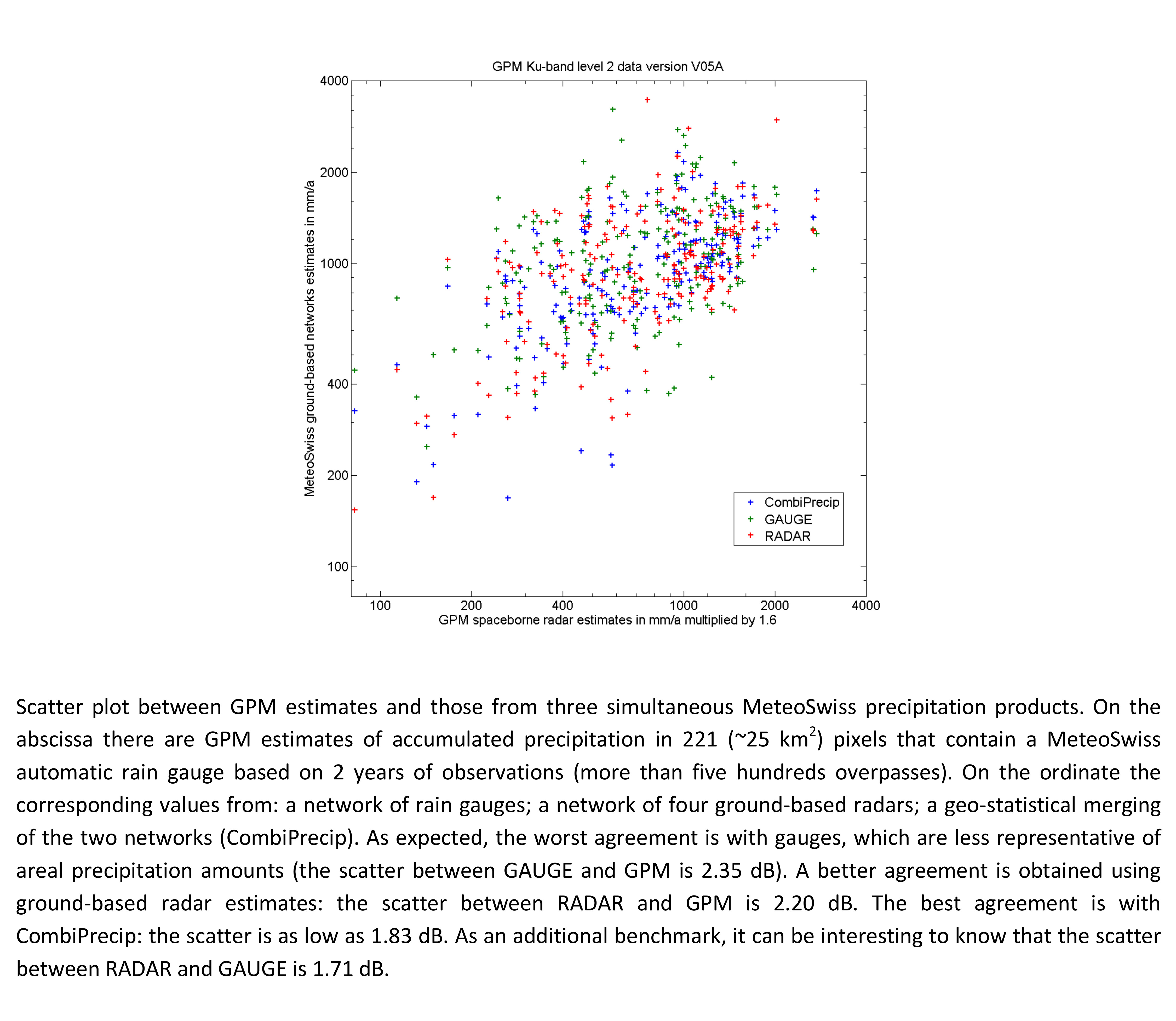
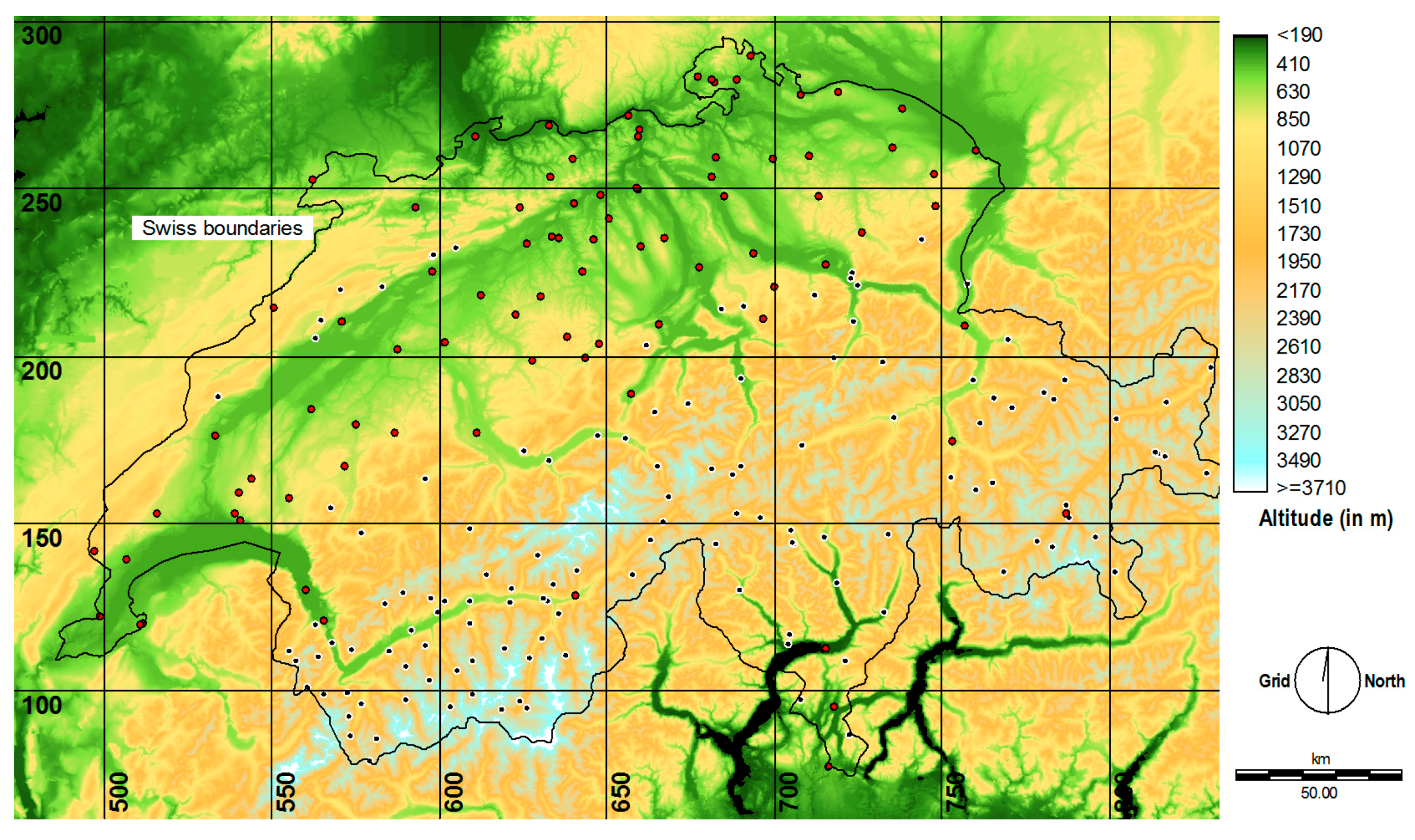
2.5. Brief Description of the Study Area

The study area is a rectangular region of 360 × 240 km around Switzerland. Figure 1 shows a digital elevation map (using the Swiss conformal mapping, CH1903) of this 86,400 km2 area, which is roughly twice the size of the Switzerland. It is straightforward and intuitive to have an idea of the minimum height of visibility from space, which is several hundred meters above the highest mountain within the ~20 km2 GPM circular pixel. To derive the actual height of visibility (see [5], Section 2.2, p. 2238 for a detailed definition) of ground based radars, one needs a digital elevation model (DEM), the exact scan strategy, and a radar simulator like [6] or [41]. Figure S1 in the Supplementary Material shows the height of visibility (geometric optics approach) for the MeteoSwiss network based on four radars (we make the simplification that exactly four radars were available during the whole study period). As a consequence of the simplifying geometric optics approach (according to which the angular resolution is much better than the DEM pixel, which is not the case in reality), there is an abundance of narrow radial features, so that it is easy to identify the location of the four radars. Figure 1 also shows the gauge locations, all of which are inside Switzerland. In the present note, the qualitative comparison (see Section 4 and figures in the Supplementary Material) refers to the whole rectangular area: it involves RADAR, GPM, and CombiPrecip. The quantitative comparison is based on 221 sites inside the Swiss territory (see Section 3) and involves GAUGE precipitation products, too.

2.6. Integration in Time, Areal Average Precipitation, and Spatial Distrubution of 2-Year Amounts in Switzerland

As stated in the introduction, integration in time is a possible remedy to smooth out the huge differences among the various precipitation products described in detail in Section 2.1, Section 2.2, Section 2.3 and Section 2.4. For GPM, this simply means adding (and counting) all available observations over each gauge. For the MeteoSwiss products, we add (and count) the measured values for the acquisition times that contain the overpasses; note that the GAUGE temporal resolution is 10 min, while the RADAR temporal resolution is 5 min. The hourly accumulations of CombiPrecip are disaggregated in twelve 5 min maps using the temporal information of RADAR, as described in [22] (Section 4.4, p. 1108); then, the corresponding nearest in time 5 min estimate is used. The total rainfall accumulation derived in such a way is based on the assumption of a constant precipitation rate in 5 min.
Regarding the spatial support, which is an important cause of difference among the various devices for estimating precipitation amounts, the half-power-beam wide GPM cells at the nadir have an area of roughly 20 km2. Only GPM cells that contain a gauge are considered, and the rest are discarded. For upscaling, RADAR and CombiPrecip pixels are simply averaged (in linear units of precipitation amounts) over the 25 km2 area centered on each gauge (i.e., approximately matching the GPM measurements in spatial scale). In [42] (Figure 4, p. 1004) it is shown that an upscaling based on the convolution between the Gaussian antenna radiation pattern of the spaceborne radar and the 1 km precipitation field would give better agreement; hence, we know that the scores relating GPM to RADAR and CombiPrecip are slightly pessimistic because the upscaling technique is based on the simple average of 25 pixels centered on the gauge, rather than on matching the GPM cells. GAUGE measurements are point measurements, and, as stated, the gauge cross section is 200 cm2.
Once these 2 year amounts have been derived, it is straightforward to compare the bias of GPM to that of other products. By looking at the first line of Table A1 in [25], one clearly expects a relatively large GPM underestimation with respect to RADAR (in [25] a “double-conditional” bias is presented: only estimates simultaneously larger than 0.15 mm/h from both radars are taken into account). Here we present the “overall bias”, which means that all available observations (including null values of one product while the other one was reporting precipitation, and vice versa) are taken into account. GPM overall underestimation with respect to RADAR results to be −3.0 dB, which means that, above the 221 selected pixels, only half of the total precipitation estimated by the RADAR product was estimated by GPM. Knowing that RADAR underestimation with respect to GAUGE during the whole 2014 and 2015 period was on the order of −0.9 dB, one expects a larger GPM underestimation with respect to GAUGE. This is in fact the case: GPM overall underestimation with respect to GAUGE was found to be −3.4 dB. Note that the −0.9 dB figure is based on 288 (144) RADAR (GAUGE) observations per day. If the temporal resolution of GPM were 10 min, we would have approximately 105 thousand samples in two years; instead, there are just 528 overpasses. Using the GAUGE network as a reference, one can evaluate whether 528 overpasses are representative, at least to characterize the average annual precipitation in Switzerland. Using all 105 thousand samples, one gets an average annual precipitation of approximately 1200 mm/a (GAUGE network); using only the 528 nearest in time GAUGE observations and averaging the 221 rain gauge values, one gets approximately 1100 mm/a. In this paper, the annual estimates are simply derived by multiplying the sum of the instantaneous amounts (expressed in mm/h) by 24 × 365 and dividing the result by the number of available overpasses over the 221 sites.
However, it is important to remark that the focus of this study is not on the estimate of the average precipitation in the country, but on its spatial variability. Consequently, in Section 3, the agreement is not evaluated in terms of the mean error, but rather in terms of the dispersion of the error around the mean (Section 3.2), as well as of the correlation among the various precipitation products (Section 3.1). As will be seen in Section 2.7 and Section 3, the scores used to evaluate the agreement are independent of any multiplicative compensation factor; however, for visualization purposes (scatter plots in Section 3 and Section 4; GPM, RADAR and CombiPrecip maps in the Supplementary Material file), GPM precipitation values will be multiplied by a factor of 1.6, which corresponds approximately to a 2 dB compensation.

2.7. Scatter in dB as a Measure of Dispersion of the Multiplicative Error from the Mean

It is well known that quantitative precipitation estimates derived aloft by the spaceborne precipitation radar (e.g., [25,43,44]) and the ground-based weather radar (e.g., [7,8,9,10,11,12,13]) may suffer from a significant mean field bias (typically, underestimation) with respect to in situ point measurements at the ground. Since from a radar–meteorological point of view the multiplicative nature of the error is dominant relative to the additive one, the mean error is defined as the Log-transformed ratio between the spaceborne radar total and, for instance, the GAUGE total. Once the underestimation is compensated, the goal of our evaluation is to answer the following two questions: (1) how much does the Log-transformed ratio between the GPM precipitation product and the other three MeteoSwiss products vary from site to site in Switzerland? (2) For each given weighted contribution to the average annual precipitation amount, what is the range of variability of the Log-transformed ratio between GPM and the other products? (In the latter question we are trying to be more cautious and closer to the users’ point of view).
Let be x the Log-transformed ratio in dB of the precipitation product under test, Ptest, with respect to the reference product, Pref in the formula:
x = 10   L o g ( P t e s t P r e f )
A robust score for the dispersion of x, which represents the variability in Switzerland of the multiplicative error, could simply be the median absolute deviation from the median (MADM), as defined in Equation (5) of [25]. This score adequately answers the first question. Furthermore, in cases where the cumulative distribution function (CDF) of x is symmetric, then the MADM is half of the widely used interquartile range. However, MADM is resilient along the abscissa but not over the ordinate (where the normalized CDF ranges from 0 to 1). The idea is that an ill-defined ratio that results from two small precipitation amounts should receive much less weight than an event characterized by much larger precipitation amounts. Bearing this in mind, in conceiving the score called scatter, each ratio data pair receives on the y axis a normalized contribution which is proportional to its contribution to the total amount [26,38] (Section 4.1, pp. 53–54). The introduction of a weighted CDF is a crucial concept in the definition of the scatter. The scatter is defined as half the distance between the 16% and 84% percentiles of the weighted CDF. An example of a weighted CDF is shown in [45] (Figure 3). There, GAUGE is the reference, while RADAR is the product under test; this is relevant because an important aspect in the definition of scatter is that the weights, which affect the steps on the ordinate axis, are proportional to the amounts of the reference. Consequently, in relation to the present analysis, the scatter of GPM with respect to the that of the other three products is different from the scatter of each of the products with respect to that of GPM. Both the scatter and MADM are independent of any multiplicative factor that could affect the retrieved precipitation estimates. This means that both scatter and MADM are orthogonal to the bias. In addition, they are expressed in dB, like the bias.

3. Results

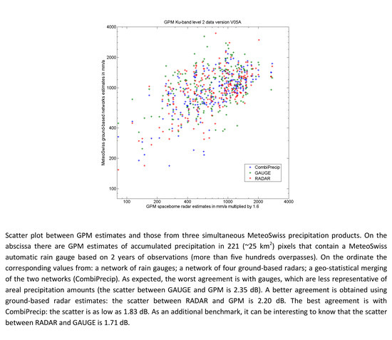
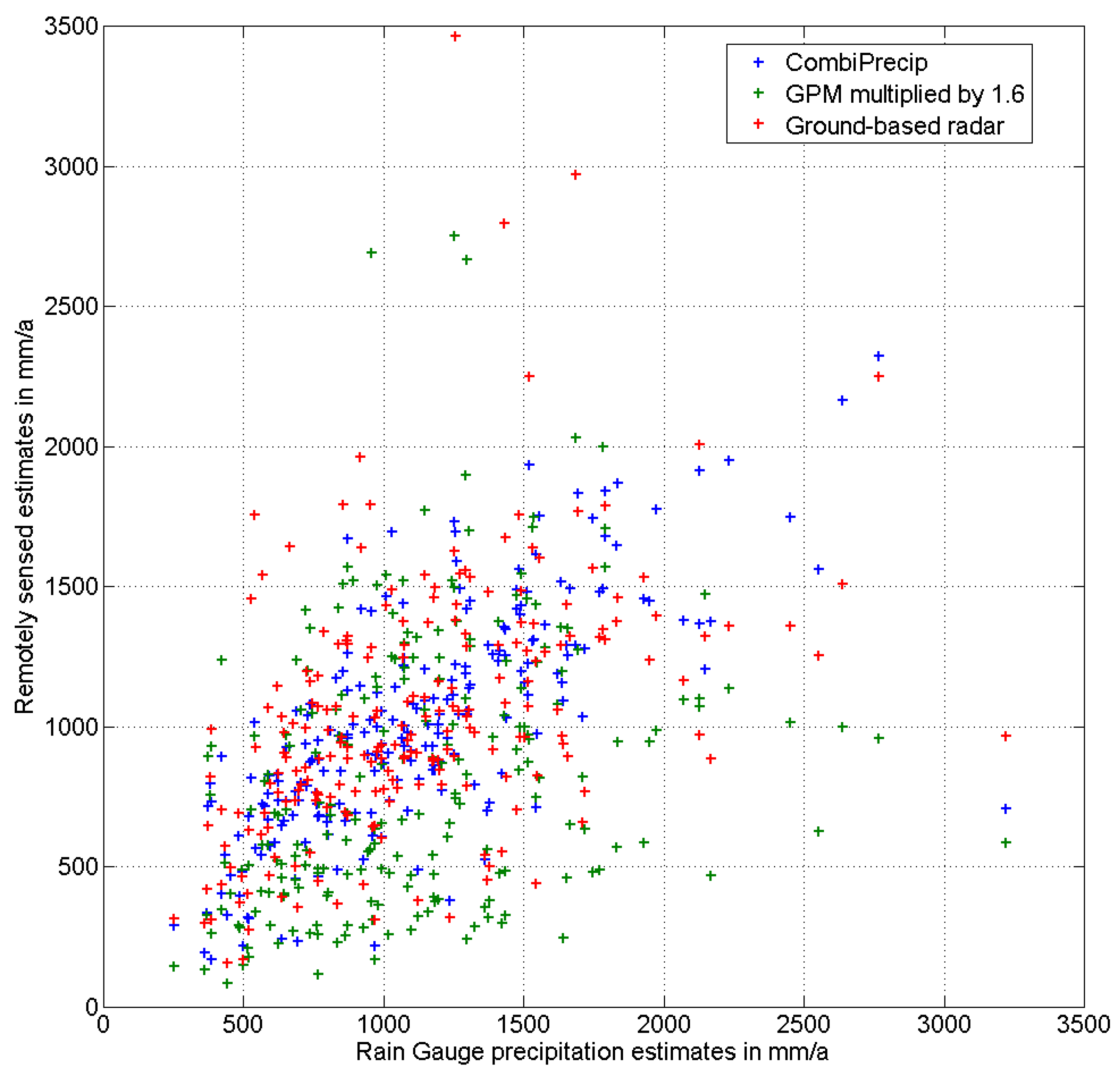
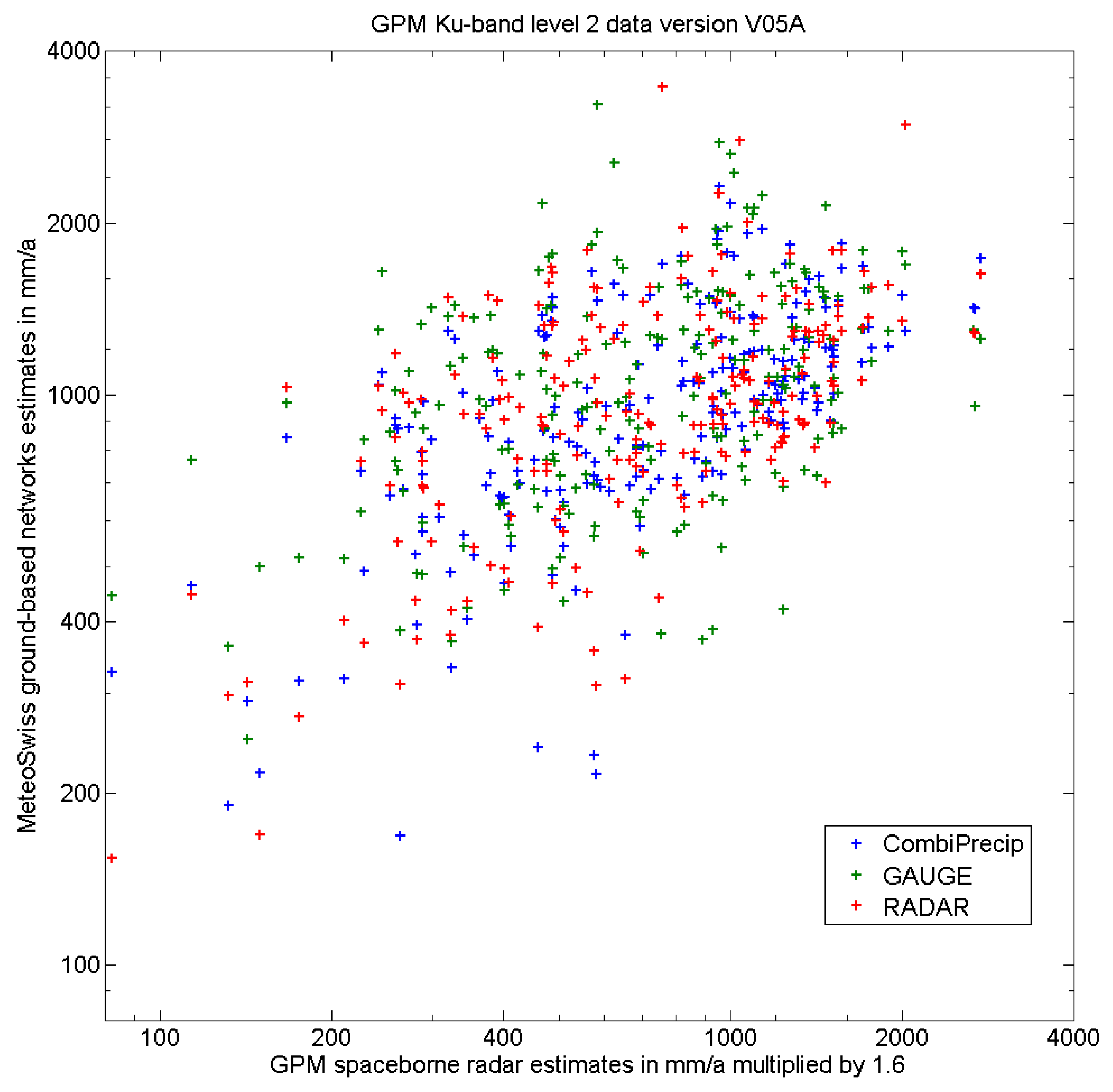
3.1. Correlation between Spaceborne Radar Amounts and the Three MeteoSwiss Products Amounts

For correlation, the standard Pearson correlation coefficient is used. It is applied to 221 total precipitation amounts at rain gauge sites (219 degrees of freedom); results are shown in Table 1. The first and third line show the values after the precipitation amounts were Log-transformed in order to minimize the influence of the asymmetry of the distributions of total precipitation amounts. In these cases, the probability distribution functions are close to being normal as a result of the monotonic logarithmic transformation. In both cases, for Log-transformed and linear amounts, the outcome is clear: inside the Swiss domain (221 points out of ~1600 GPM pixels) the best correlation is between GPM and the CombiPrecip precipitation product, followed by RADAR, and, as expected, by gauges. This is valid for both versions of GPM products: V04A and V05A. Using the new version V05A, the correlation slightly increases in the case of linear amounts.
Figure 2 shows the scatterplot of the 221 Log-transformed data pairs from which the Pearson correlation coefficients were derived (first line in Table 1). The annual GPM estimates (augmented by 2 dB) are on the abscissa, while the three MeteoSwiss precipitation estimates are on the ordinate; Combiprecip values are in blue, RADAR in red, and GAUGE in green. It can easily be observed that the blue marks are the one closest to a straight regression line (best correlation), while the green ones show the worst correlation. Among the green marks, one is of particular interest, namely the one with the largest precipitation amount: 76.8 mm/h equivalent (actually, 12.8 mm/10 min) during 212 wet GPM overpasses, which corresponds approximately to an annual estimate of 3173 mm (76.8 × 24 × 365/212). This ~3170 mm/a in situ point estimate was derived using gauge measurements acquired at the “Passo del Gran San Bernardo” at 2472 m altitude (GSB, using MeteoSwiss nomenclature). It is a high altitude pass connecting Switzerland (Valais) to Italy (Valle d’Aosta), where precipitation measurements are challenging, especially when there is still snow. The snow is often blown into the gauge by a strong wind which is accelerated because of the Venturi effect. More details and in depth analysis will be given in Section 4; here, it is enough to underline that the 600/1.6 mm/a GPM estimate should not be compared with the 3170 mm/a estimate, but rather with a smaller value. At the moment, at MeteoSwiss we have no quantitative estimate of the amount of false precipitations blown by the wind. However, since the beginning of the year, a second rain gauge has been installed at a better site, and comparison analyses are ongoing; we are confident that we will be able to give a preliminary answer to this interesting question in a couple of years, assuming that the amounts for 2017 and for the subsequent years are sufficiently representative of the past years.

3.2. Dispersion of the Difference from the Mean Among the Various Precipitation Products

From Section 2 in this note and Table A1 in [25], one can read that the GPM “overall bias” (“double-conditional bias”) with respect to RADAR is −2.9 (−2.2 dB). The GPM “overall bias” with respect to GAUGE is even larger: −3.3 dB. However, in this Section 3.2, we evaluate the agreement between GPM and three different MeteoSwiss products using scores that are independent, namely, the Scatter (see Section 2.7) and the widely known MADM. Table 2 shows the values of the scatter in dB between GPM and each of the three MeteoSwiss products. Using the new version V05A, there is an improvement in terms of dispersion of the error around the mean in all cases except for CombiPrecip, when it is used as a reference. The general interpretation of the outcome is straightforward: independently of the user’s point of view (the weights on the y axis), the MeteoSwiss precipitation product that spatially best agrees with the GPM estimates is CombiPrecip. This is followed by the ground-based radar product, while, as expected, the poorest agreement is found with the gauge amounts. This result is confirmed by the MADM, whose values for the GPM version V05A (V04A) are 1.47 (1.61) dB, 1.80 (1.83) dB, and 1.91 (1.94) dB, respectively. Another important conclusion is that the new GPM V05A product agrees better than the previous version with MeteoSwiss precipitation products.
Hence, we conclude that, given the spatial variability of the precipitation fields as observed by GPM over 221 sites in Switzerland, the best precipitation product is CombiPrecip because, on the one hand, it has the best correlation, and, on the other hand, it shows the smallest dispersion of the multiplicative differences around the mean annual precipitation value. As a further benchmark, the scatter between RADAR and GAUGE estimates for the 221 amounts is 1.71 (1.67) dB when GAUGE (RADAR) is used as a reference.

4. Discussion

In this Section, we further discuss the quantitative agreement among the four precipitation products in the 221 sites where gauge measurements are available; then, we analyze the qualitative agreement among GPM, RADAR, and CombiPrecip in the described study area (360 × 240 km2), with special focus on the Swiss territory.
We first complete the visualization of the scatterplots associated with the correlation coefficient values that are shown in Table 1 and discussed in Section 3. In this respect, Figure 2 shows the Log-transformed annual precipitation estimates and Figure 3 shows the original linear values. Please note that, with respect to Figure 2, we have changed the independent variable point of view, and thus, in Figure 3, the gauge amounts are reported on the abscissa, while GPM (augmented by 2 dB), RADAR, and CombiPrecip are shown on the ordinate. We have opted for GAUGE values on the abscissa to check the reliability and representativeness of the values corresponding to the large gauge amounts collected every 10 min that were acquired during the first 2 years of activity of the GPM Core Observatory satellite. As stated in Section 2, these 528 samples are synchronous with the GPM overpasses over the Swiss territory and represent a “random” subsample of 0.5% of all available samples. Using all samples, the rainiest site (ROE, 1896 m altitude) shows ~2500 mm/a, while the second and third rainiest sites (SAE, 2502 m; GSB, 2472 m) show ~2350 mm/a and ~2150 mm/a, respectively. As can be easily seen in Figure 1 and Figure 2, using the GPM-synchronous 528 samples, the rainiest site is found to be GSB (~3220 mm/a) followed by Saentis (SAE, ~2770 mm/a). Figure 2 also shows that while the RADAR and CPC underestimation at the SAE site are still “acceptable”, at the GSB site they are not. All three products suggest that the rain gauge is not reliable at that site. This fact is well known at MeteoSwiss: for instance, the correlation coefficient between 6589 wet–wet RADAR–GAUGE hourly amounts during the period 2005–2009 is as low as 0.133. Additional investigations have suggested that this rain gauge site is far from being ideal. At the end of 2016, a new rain gauge was installed in a better position (~1 km away from the old site). Preliminary comparisons between the radar and the two gauge estimates seem to confirm that the site of the new gauge is much better. Thanks to GPM (see Figure 2), MeteoSwiss has an additional confirmation of the problem at GSB. It is also worth noting that the correlation and scatter values presented in Section 3 are not sensitive to the GSB data pair; rather, they are reasonably resistant. In fact, by eliminating GSB, the correlation coefficient between GAUGE and GPM increases from 0.403 to 0.411 (Log values) and from 0.290 to 0.312, and the scatter decreases from 2.84 dB to 2.78 dB using GAUGE as a reference. As expected, the elimination of the GSB site does not influence the agreement of GPM with RADAR or with CombiPrecip.
The performance of the various precipitation products can also be evaluated using additional scores, like the Root Mean Square Error (RMSE), the Heidke skill score (HSS), and the Nash-Sutcliffe (NS) efficiency. Table 3 shows the values of the root mean square difference (“error”) between GPM and the three MeteoSwiss precipitation products. The results are identical to those obtained with the correlation coefficient (Table 1) and the scatter (Table 2): the best agreement is observed with CombiPrecip, followed by the ground-based radar, and finally the gauge network. Note that the RMSE can be decomposed in two orthogonal contributions: the square of the mean difference and the variance of the differences. Original GPM values give a significant mean error component because of the large underestimation. Therefore, in the second row of Table 3 we also show the values after a posterior adjustment of +2 dB, which is the same factor used in Figure 1 and Figure 2. However, due to the relatively poor correlations (see Table 1, line 2) between GPM and the three products, this causes not only a reduction of the squared mean difference, but also an increase of the variance of the difference. Nevertheless, a compensation of 2 dB still gives a better RMSE than the one obtained with the original GPM estimates, as can be seen by comparing the values in the two lines of Table 3 and Table 4. An adjustment of 3 dB brings the square of the mean difference to zero, but causes an enormous increase of the variance of the difference, so that the RMSE becomes even larger than the one obtained with the original (underestimated) GPM estimates.
Similar results can be seen in Table 4, with a slight improvement when using the new version of the GPM-DPR level-2 data, namely, V05A.
Table 5 shows the values of the Heidke Skill Score in the case of a polychoric metrics; in particular, we have opted for a 4 × 4 contingency table, with the GPM estimates augmented by 2 dB along the columns, and (alternatively) the three MeteoSwiss products along the rows. The three thresholds used to define the four categories are: 650, 850, and 1250 mm/a. These are exactly the same values used in Figures S2 (GPM estimates), S3 (RADAR estimates), and S4 (CombiPrecip estimates). The HSS values confirm the results obtained using correlation, scatter, MADM, and RMSE: the best agreement is observed between GPM and CombiPrecip, followed by RADAR and GAUGE. In all cases, the GPM version V05A performs better than the V04A.
The definition of the NS efficiency is based on a regression through the origin, instead of an ordinary least-squares regression (like the one used to derive the correlation coefficients shown in Table 1). The ratio between the RMSE and the standard deviation of the reference is the crucial quantity in the definition of the NS efficiency, which is one minus such a ratio. A performance evaluation based on the NS efficiency confirms what was evidenced by the other scores: the best agreement is between GPM and CombiPrecip. Again, results are slightly better when data from the GPM version V05A are used instead of those from the V04A version. In addition, all the five scores used provide the same ranking picture: the estimates of accumulated precipitation from space during the first 2 years of GPM life in 221 Swiss sites agree better with those of the CombiPrecip product, followed by the those of RADAR and then, as expected, those of GAUGE. The extensive statistical analysis presented so far also shows that the GPM version V05A agrees better than the V04A version with the three MeteoSwiss precipitation products.
So far the quantitative analysis was based on 221 total amounts and 4 precipitation products. Three products, however, carry continuous spatial information regarding the precipitation fields in all the 3456 pixels (25 km2) of the study area. The corresponding images for Log-transformed and linear total precipitation amounts are shown in Figures S3 and S4, respectively: 528 overpasses are already enough to highlight several climatological features of the area surrounding the northern part of the Western Alps (from Monte Bianco to Ortler and Piz Murnin) and the Jura mountains. By comparison with Figure S1, it can clearly be seen that orography strongly affects precipitation in the study area. The dominant weather pattern across much of Switzerland is characterized by a westerly-northwesterly wind bringing precipitation that falls primarily on the northwestern side of the Alps. Another dominant pattern on the southern side of the Alps (Piemonte, Canton Ticino, Lombardia) is also clearly visible, although it appears more “convective” (there are several high precipitation patterns composed of just few pixels, corresponding to areas that are smaller than 100 km2). This southern part of the Alps tends to get its precipitation from a different weather pattern (characterized by a southerly wind from the Mediterranean), resulting in high amounts of precipitation on the western or central Prealps or Alps, depending on the direction (and strength) of the winds in the low (typically south–easterly) and upper (typically south–westerly) levels [46]. In the southwestern Alps and in the surrounding flatlands and hills, autumn is the season in which the heaviest daily rainfalls occur [47]. This fact has long been known: the description of these “late-summer” Mediterranean storms can be found even in "Naturalis Historia" by the Roman author Plinius. There is then another area of higher precipitation in the smaller Jura Mountains in the northwest of Switzerland, which form the first significant mountain range encountered by the westerly fronts, hence generating a strong orographic enhancement of precipitation.
It is interesting to note (Table 6) the values of the Coefficient of Variation (CoV, relative dispersion) that characterizes the probability distribution functions of the linear precipitation amounts (3456 pixels) over the study area (86,400 km2). It is observed that GPM presents the largest value, followed by RADAR, while CombiPrecip presents the smallest value. This is also the case when dividing the study area in two (roughly equal) parts, inside and outside Switzerland (lines 2 and 3), and it is caused by an increased underestimation tendency of GPM with increasing orographic complexity. Consequently, the difference in the relative dispersion between GPM and RADAR (or CombiPrecip) is larger inside Switzerland, where there are more mountains. To further explore the effect of an increasing orographic complexity, we divided the data set in two parts, i.e., complex and flat terrain, using the same strategy and threshold as in [25] (Section 2.d, p. 1253). It can be observed that the CoV characterizing 135 sites in complex terrain is larger than the CoV in non-complex terrain. The stratification upon altitude also shows the quite different level of underestimation between GPM and RADAR or CombiPrecip. Using 135 sites (pixels) in complex terrain, in fact, the Mean Field Bias is −3.8 dB with respect to the RADAR, and −3.5 dB with respect to CombiPrecip. Using 86 sites in non-complex terrain, the underestimation is −0.9 dB with respect to both products. This confirms findings by Speirs et al. [25] using RADAR as reference: both detection and estimation performance of GPM over Switzerland are significantly better in flatter than in complex terrain.
As a result of 2 years of GPM observations, a new, completely independent QPE product is now available for MeteoSwiss. In this note, GPM total amounts have been compared in detail with those of the other MeteoSwiss QPE products. Unfortunately, the GPM estimates are less reliable just in those high altitude areas where MeteoSwiss estimates are also more uncertain or absent (GAUGE). Consider, for instance, that there are only three MeteoSwiss gauges (~1.4% of the total) at an altitude over 2500 m (the altitude of the above mentiones SAE and GSB sites), while more than 10% of the Swiss territory is at an altitude over 2500 m. There is a clear need to improve the knowledge of the complex precipitation fields at such high altitudes. To conclude, a key point is whether 528 GPM overpasses (a few hundred of them with some wet pixels in Switzerland) are sufficient to derive an accumulation product able to discriminate which MeteoSwiss precipitation product shows the more realistic spatial variability of precipitation. Thanks to the experience gained in mountainous regions in the southeastern Mediterranean [43,44] and western Alps [25], we are confident that this is the case. However, it will be necessary to extend the analysis for a few more years. To this end, it is planned, in fact, to analyze data from 2016, hence fully exploiting the observations from the recently installed ground-based radar in the Eastern part of the country. Further extension to 2017 and subsequent years will certainly make the data set more robust and representative, especially in those areas where the contribution to the generation of precipitation was caused more by convective instability than by baroclinic instability. Consider, for example, that eight years of spaceborne radar were used in cases where the TRMM-PR level 2 data alone were used to characterize precipitating convective systems in the southeastern Asia [48], as well as their regional, seasonal, and diurnal variations [49].
Just as the TRMM Precipitation Radar was used in the last 20 years, the GPM-DPR is primarily intended to be used as the calibration basis for radiometer-derived global precipitation products [1]. The GPM core satellite, in fact, carries on board not only the active DPR, but also the passive microwave radiometer called GMI [50]. As such, it is important that the DPR provides a reliable reference in as many circumstances as possible. The work presented here is focused on the performance of the DPR for quantitative precipitation estimations in complex terrain (the western Alps). DPR performance is found to be remarkably better in flatter terrain (the Swiss plateau) than in complex terrain. In turn, this may affect passive radiometer estimates, which are known to be more problematic over complex terrain than in flat areas (e.g., [51]). Furthermore, it has been recently shown [52] that radiometers estimates over mountainous terrain could be improved through a simple parametrization that accounts for orographic enhancement. Hence, our future analysis will be carried out also as a function of the complexity of orography (complex vs. flatter terrain).

5. Conclusions

Switzerland is a unique and ideal ground validation site for comparing spaceborne weather radar level 2 precipitation estimates (GPM, Section 2.1) with other different precipitation products, as the mountainous and relatively small (~41,000 km2) country is equipped with a network of telemetered, automatic rain gauges (GAUGE, Section 2.3), and with a state-of-the-art dual-polarization network of weather radars (RADAR, Section 2.2). A third and innovative MeteoSwiss precipitation product is available (CombiPrecip, Section 2.4), which is a real-time geostatistical merging of RADAR and GAUGE. To the best of the authors’ knowledge, there is no existing published work examining the GPM-DPR precipitation product and three other different precipitation products in mountainous terrain. On average, GPM underestimates precipitation amounts by −3.0 dB with respect to RADAR, and by −3.4 dB with respect to GAUGE.
Ground-based and spaceborne radars provide a complementary view of the complex and highly variable precipitation fields: the former measures precipitations from a lateral direction, while the latter looks at the precipitation fields from the top. The radar backscattering volume increases with the square of the range. Consequently, the changes in resolution of the GPM radar are almost negligible, since its measurements originate from similar distances of 400–420 km over the whole swath. On the contrary, the sampling volume of the ground-based radar changes significantly, since it has to measure precipitation from close to large distances. Hence, the GPM can be used as a reference to evaluate the proper spatial variability of both the RADAR and the CombiPrecip products, since the former is used as an external drift to derive the latter in the geostatistical merging based on GAUGE kriging. This explains why, in this note, not only an evaluation is made of the GPM level 2 estimated surface precipitation product against syncrhonous estimates from the MeteoSwiss RADAR, GAUGE ,and Combiprecip products, but GPM is also used as a reference to evaluate the dispersion of the multiplicative difference between each MeteoSwiss products and an unbiased version of the GPM-derived field.
The evaluation of the GPM level 2 precipitation product in the Swiss complex terrain is of interest for those who plan to use GPM in other mountainous areas. The GPM core satellite is, in fact, adding significant new coverage to mountainous areas, especially in poorly instrumented parts of the world and at latitudes not previously covered by TRMM. This study shows that, in terms of average precipitation, a clear underestimation by GPM (with respect to the dense ground-based radar or the gauge networks) can be expected also in other mountainous areas of the world. Regarding the dispersion of the GPM error around the mean, even by integrating 2 years of overpasses, the overall scatter associated with the high-resolution DPR cells (20 km2) is of the order of 2.6 dB. This figure represents an overall post facto assessment, and it is simply a quantitative assessment of the scatter of the differences between the DPR and the other three ground-based references, namely, the rain gauge network (2.8 dB), the weather radar network (2.6 dB), and a geostatistical combination (CombiPrecip) of these two ground-based networks (2.4 dB).
Regarding the use of GPM for evaluating the performance of the three MeteoSwiss products, the smallest dispersion is observed between GPM and CombiPrecip (scatter ~1.8 dB), followed by GPM and RADAR (scatter ~2.2 dB), whereas a larger disagreement was found between GPM and GAUGE (scatter ~2.4 dB). GPM confirms that, for precipitation mapping in the Alpine region, the best results are obtained by combining ground-based radar and rain-gauge measurements using a geostatistical approach.

Supplementary Materials

One file with four additional images is available online at www.mdpi.com/2072-4292/9/11/1147/s1. Figure S1 shows the Effective Height of Visibility of the weather radar network. Figure S2 shows estimate of annual precipitation amounts derived using MeteoSwiss weather radar observations synchronous with the GPM satellite overpasses. Figure S3 shows the corresponding GPM estimates. Figure S4 shows the corresponding estimates based on the MeteoSwiss product called CombiPrecip, which is a geostatistical merging of synchronous rain gauge measurements and ground-based radar observations.

Acknowledgments

The authors would like to thank the Swiss Confederation. The GPM data were provided by the NASA DAAC at the Goddard Space Flight Center. The authors would like to thank the anonymous reviewers and the academic editor for helpful and stimulating comments.

Author Contributions

P.S., M.G. and A.B. conceived and designed the comparisons among the four different precipitation products; P.S. conceived and programmed all the routines to extract and process satellite, ground-based radar, gauge, and CombiPrecip data; he conceived and developed the routines for georeferencing the GPM latitude/longitude cells on the Swiss conformal Cartesian grid used by MeteoSwiss; P.S. and M.G. contributed analysis tools and materials; M.G. analyzed the data and prepared the figures; he also prepared figures in Supplementary File 1, together with U.H. M.G. wrote the paper after feedback, suggestions, comments, and changes by P.S., A.B., U.H., and U.G.; the paper was corrected and checked for English usage by P.S. and A.B.

Conflicts of Interest

The authors declare no conflict of interest.

References

  1. Neeck, S.P.; Kakar, R.K.; Azarbarzin, A.A.; Hou, A.Y. Global Precipitation Measurement (GPM) launch, commissioning, and early operations. In Sensors, Systems, and Next-Generation Satellites XVIII; Meynart, R., Neeck, S.P., Shimoda, H., Eds.; International Society for Optical Engineering: Bellingham, WA, USA, 2014. [Google Scholar]
  2. Houze, R., Jr. Orographic effects on precipitating clouds. Rev. Geophys. 2012, 50. [Google Scholar] [CrossRef]
  3. Germann, U.; Boscacci, M.; Gabella, M.; Sartori, M. Radar design for prediction in the Swiss Alps. Meteorol. Technol. Int. 2015, 4, 42–45. [Google Scholar]
  4. Germann, U.; Joss, J. Operational measurement of precipitation in mountainous terrain. In Weather Radar: Principles and Advanced Applications; Meischner, P., Ed.; Springer: Berlin, Germany, 2004; pp. 52–77. [Google Scholar]
  5. Gabella, M.; Joss, J.; Perona, G. Optimizing quantitative precipitation estimates using a non-coherent and a coherent radar operating on the same area. J. Geophys. Res. 2000, 105, 2237–2245. [Google Scholar] [CrossRef]
  6. Gabella, M.; Perona, G. Simulation of the orographic influence on weather radar using a geometric-optics approach. J. Atmos. Ocean. Technol. 1998, 15, 1486–1495. [Google Scholar] [CrossRef]
  7. Wilson, J.W.; Brandes, E.A. Radar measurement of rainfall—A summary. Bull. Am. Meteorol. Soc. 1979, 60, 1048–1058. [Google Scholar] [CrossRef]
  8. Zawadzki, I. Factors affecting the precision of radar measurements of rain. In Proceedings of the 22nd Conference on Radar Meteorology, Zurich, Switzerland, 10–13 September 1984; pp. 251–256. [Google Scholar]
  9. Collier, C.G. Accuracy of rainfall estimates by radar, part I, Calibration by telemetering rain gauges. J. Hydrol. 1986, 83, 207–223. [Google Scholar] [CrossRef]
  10. Koistinen, J.; King, R.; Saltikoff, E.; Harju, A. Monitoring and assessment of systematic measurement errors in the NORDRAD network. In Proceedings of the 29th Conference on Radar Meteorology, Montreal, QC, Canada, 12–16 July 1999; pp. 765–768. [Google Scholar]
  11. Joss, J.; Waldvogel, A. Precipitation measurements and hydrology: A review. In Radar Meteorology; Atlas, D., Ed.; American Meteorological Society: Boston, MA, USA, 1990; pp. 577–606. [Google Scholar]
  12. Gabella, M. Improving operational measurement of precipitation using radar in mountainous terrain—Part II: Verification and Applications. IEEE Geosci. Remote Sens. Lett. 2004, 1, 84–89. [Google Scholar] [CrossRef]
  13. Kitchen, M.; Blackall, R.M. Representativeness errors in comparisons between radar and gauge measurements of rainfall. J. Hydrol. 1992, 134, 13–33. [Google Scholar] [CrossRef]
  14. Austin, P.M. Relation between measured radar reflectivity and surface rainfall. Mon. Weather Rev. 1987, 115, 1053–1070. [Google Scholar] [CrossRef]
  15. Zawadzki, I. On radar-raingauge comparison. J. Appl. Meteorol. 1975, 14, 1430–1436. [Google Scholar] [CrossRef]
  16. Brandes, E.A. Optimizing rainfall estimates with the aid of radar. J. Appl. Meteorol. 1975, 14, 1339–1345. [Google Scholar] [CrossRef]
  17. Creutin, J.D.; Dekrieu, G.; Lebel, T. Rain measurement by raingauge-radar combination: A geostatistical approach. J. Atmos. Ocean. Technol. 1987, 5, 102–114. [Google Scholar] [CrossRef]
  18. Krajewski, W.F.; Georgakakos, K.P. Cokriging radar-rainfall and rain gauge data. J. Geophys. Res. 1987, 21, 764–768. [Google Scholar]
  19. Seo, D.J.; Krajewski, W.F.; Bowles, D.S. Stochastic interpolation of rainfall data from rain gauges and radar using cokriging. 1. Design of Experiments. Water Resour. Res. 1990, 26, 469–477. [Google Scholar]
  20. Gabella, M.; Notarpietro, R. Improving operational measurement of precipitation using radar in mountainous terrain—Part I: Methods. IEEE Geosci. Remote Sens. Lett. 2004, 1, 78–83. [Google Scholar] [CrossRef]
  21. Schuurmans, J.M.; Bierkens, M.F.P.; Pebesma, E.J.; Uilenhoet, R. Automatic prediction of high-resolution daily rainfall fields for multiple extents: The potential of operational radar. J. Hydrometeorol. 2007, 8, 1204–1224. [Google Scholar] [CrossRef]
  22. Sideris, I.V.; Gabella, M.; Erdin, R.; Germann, U. Real-time radar-rain-gauge merging using spatio-temporal co-kriging with external drift in the alpine terrain of Switzerland. Q. J. R. Meteorol. Soc. 2014, 140, 1097–1111. [Google Scholar] [CrossRef]
  23. Villarini, G.; Mandapaka, P.V.; Krajewski, W.F.; Moore, R.J. Rainfall and sampling uncertainties: A rain gauge perspective. J. Geophys. Res. 2008, 113, 1–12. [Google Scholar] [CrossRef]
  24. Gabella, M.; Duque, D.; Notarpietro, R. Comparing meteorological spaceborne and ground-based radars: Optimal satellite overpass distance from the ground-based radar site. Int. J. Remote Sens. 2012, 32, 322–330. [Google Scholar] [CrossRef]
  25. Speirs, P.; Gabella, M.; Berne, A. A comparison between the GPM dual-frequency precipitation radar and ground-based radar precipitation rate estimates in the Swiss Alps and Plateau. J. Hydrometeorol. 2017, 18, 1247–1269. [Google Scholar] [CrossRef]
  26. Condom, T.; Rau, P.; Espinoza, J.C. Correction of TRMM 3B43 monthly precipitation data over the mountainous area of Peru during the period 1998–2007. Hydrol. Process. 2011, 25, 1924–1933. [Google Scholar] [CrossRef]
  27. Mourre, L.; Condom, T.; Junquas, C.; Lebel, T.; Sicart, J.; Figueroa, R.; Cochachin, A. Spatio-temporal assessment of WRF, TRMM and in situ precipitation data in a tropical mountain environment (Cordillera Blanca, Peru). Hydrol. Earth Syst. Sci. 2016, 20, 125–141. [Google Scholar] [CrossRef]
  28. Nastos, P.; Kapsomenakis, J.; Philandras, K. Evaluation of the TRMM 3B43 gridded precipitation estimates over Greece. Atmos. Res. 2016, 169, 497–514. [Google Scholar] [CrossRef]
  29. Gabella, M.; Michaelides, S.; Constantinides, P.; Perona, G. Climatological validation of TRMM Precipitation Radar monthly rain products over cyprus during the first 5 years (December 1997–November 2002). Meteorol. Z. 2006, 15, 559–564. [Google Scholar] [CrossRef]
  30. Prasetia, R.; RahmanAs-syakur, A.; Osawa, T. Validation of TRMM Precipitation Radar satellite data over Indonesian region. Theor. Appl. Climatol. 2013, 112, 575–587. [Google Scholar] [CrossRef]
  31. Gabella, M.; Sartori, M.; Boscacci, M.; Germann, U. Vertical and Horizontal Polarization Observations of Slowly Varying Solar Emissions from Operational Swiss Weather Radars. Atmosphere 2015, 6, 50–59. [Google Scholar] [CrossRef]
  32. Huuskonen, A.; Holleman, I. Determining weather radar antenna pointing using signals detected from the Sun at low antenna elevations. J. Atmos. Ocean. Technol. 2007, 24, 476–483. [Google Scholar] [CrossRef]
  33. Holleman, I.; Huuskonen, A.; Kurri, M.; Beekhuis, H. Operational monitoring of weather radar receiving chain using the Sun. J. Atmos. Ocean. Technol. 2010, 27, 159–166. [Google Scholar] [CrossRef]
  34. Vollbracht, D.; Sartori, M.; Gabella, M. Absolute dual-polarization radar calibration: Temperature dependence and stability with focus on antenna-mounted receivers and noise source-generated reference signal. In Proceedings of the 8th European Conference on Radar in Meteorology and Hydrology (ERAD2014), Garmisch-Partenkirchen, Germany, 1–5 September 2014. [Google Scholar]
  35. Gabella, M.; Sartori, M.; Progin, O.; Germann, U. Acceptance tests and monitoring of the next generation polarimetric weather radar network in Switzerland. In Proceedings of the 2013 International Conference on Electromagnetics in Advanced Applications (ICEAA), Torino, Italy, 9–13 September 2013. [Google Scholar]
  36. Gabella, M.; Boscacci, M.; Sartori, M.; Germann, U. Calibration accuracy of the dual-polarization receivers of the C-band Swiss weather radar network. Atmosphere 2016, 7, 76. [Google Scholar] [CrossRef]
  37. Joss, J.; Lee, R. The application of radar-gauge comparisons to operational precipitation profile corrections. J. Appl. Meteorol. 1995, 34, 2612–2630. [Google Scholar] [CrossRef]
  38. Germann, U.; Galli, G.; Boscacci, M.; Bolliger, M. Radar precipitation measurement in a mountainous region. Q. J. R. Meteorol. Soc. 2006, 132, 1669–1692. [Google Scholar] [CrossRef]
  39. Germann, U.; Joss, J. Mesobeta profiles to extrapolate radar precipitation measurements above the Alps to the ground level. J. Appl. Meteorol. 2002, 41, 542–557. [Google Scholar] [CrossRef]
  40. Sideris, I.V.; Gabella, M.; Sassi, M.; Germann, U. The CombiPrecip experience: Development and operation of a real-time radar-raingauge combination scheme in Switzerland. In Proceedings of the 8th International Symposium on Hydrologic Applications of Weather Radar, Washington, DC, USA, 7–9 April 2014. [Google Scholar]
  41. Pellarin, T.; Delrieu, G.; Saulnier, G.R.; Andrieu, H.; Vignal, B.; Creutin, J.D. Hydrologic visibility of weather radar systems operating in mountainous regions: Case study for the Ardèche catchment (France). J. Hydrometeorol. 2002, 3, 539–555. [Google Scholar] [CrossRef]
  42. Gabella, M.; Michaelides, S.; Perona, G. Preliminary comparison of TRMM and ground-based precipitation radars for a European test site. Int. J. Remote Sens. 2005, 26, 997–1006. [Google Scholar] [CrossRef]
  43. Gabella, M.; Joss, J.; Michaelides, S.; Perona, G. Range adjustment for Ground-based Radar, derived with the spaceborne TRMM Precipitation Radar. IEEE Trans. Geosci. Remote Sens. 2006, 44, 126–133. [Google Scholar] [CrossRef]
  44. Gabella, M.; Morin, E.; Notarpietro, R. Using TRMM spaceborne radar as a reference for compensating ground-based radar range degradation: Methodology verification based on rain gauges in Israel. J. Geophys. Res. 2011, 116. [Google Scholar] [CrossRef]
  45. Germann, U.; Galli, G.; Boscacci, M.; Bolliger, M.; Gabella, M. Quantitative precipitation estimation in the Alps: Where do we stand? In Proceedings of the 3rd European Conference on Radar in Meteorology and Hydrology (ERAD2004), Visby, Sweden, 6–10 September 2004; pp. 2–6. [Google Scholar]
  46. Panziera, L.; Germann, U. The relation between airflow and orographic precipitation on the southern side of the Alps as revealed by weather radar. Q. J. R. Meteorol. Soc. 2010, 136, 222–238. [Google Scholar] [CrossRef]
  47. Gabella, M.; Mantovani, R. The floods of 13–16 October 2000 in Piedmont (Italy): Quantitative precipitation estimates using radar and a network of gauges. Weather 2001, 56, 337–351. [Google Scholar] [CrossRef]
  48. Romatschke, U.; Houze, R.A., Jr. Characteristics of precipitating convective systems in the Southeast Asian Monsoon. J. Hydrometeorol. 2011, 12, 3–26. [Google Scholar] [CrossRef]
  49. Romatschke, U.; Medina, S.; Houze, R.A., Jr. Regional, seasonal, and diurnal variations of extreme convection in the South Asian region. J. Clim. 2010, 23, 419–439. [Google Scholar] [CrossRef]
  50. Draper, D.W.; Newell, D.A.; Wentz, F.J.; Krimchansky, S.; Skofronick-Jackson, G.M. The Global Precipitation Measurement (GPM) Microwave Imager (GMI): Instrument overview and early on-orbit performance. IEEE J. Sel. Top. Appl. Earth Obs. Remote Sens. 2015, 8, 3452–3462. [Google Scholar] [CrossRef]
  51. Shige, S.; Kida, S.; Ashiwake, H.; Kubota, T.; Aonashi, K. Improvement of TMI rain retrievals in mountainous area. J. Appl. Meteorol. Climatol. 2013, 52, 242–254. [Google Scholar] [CrossRef]
  52. Dinku, T.; Chidzambwa, S.; Ceccato, P.; Connor, S.J.; Ropelewski, C.F. Validation of high-resolution satellite rainfall products over complex terrain. Int. J. Remote Sens. 2008, 29, 4097–4110. [Google Scholar] [CrossRef]
Figure 1. Digital Elevation Map of the (360 × 240 km2) Alpine study area centered around Switzerland. The black (red) dots show the locations of the “complex (“non-complex) terrain” rain gauges (for more details see Section 4 and [25], Section 2.d, p. 1253). The displayed Cartesian grid is coincident with the Swiss national coordinate system (CH1903), which results from a conformal mapping from the Bessel reference ellipsoid onto a longitudinal cylinder. The Swiss coordinates of the four corners (bottom-left, top-left, top-right, bottom-right) are: (473; 62), (473; 302); (833; 302), (833; 62). The corresponding Lat-Long coordinates (WGS84 datum) are: (45.6978°; 5.8083°), (47.8561°; 5.7416°), (47.8269°; 10.5509°), (45.6698°; 10.8083°).
Remotesensing 09 01147 g001
Figure 2. GPM spaceborne radar (V05A) annual precipitation estimates (multiplied by 1.6) versus the estimates from three MeteoSwiss products: RADAR (red), GAUGE (green), and the geostatistical merging of the two (CombiPrecip). Note that the multiplication of the GPM values by 1.6 on the x axis means a visual compensation of 2 dB (out of ~3 dB overall underestimation by GPM) in the log-log scatter plot.
Remotesensing 09 01147 g002
Figure 3. As in Figure 2, but using a linear (instead of logarithmic) scale for both axes and displaying GAUGE (instead of GPM) amounts on the abscissa.
Remotesensing 09 01147 g003
Table 1. Pearson correlation coefficients between the estimates of the Global Precipitation Measurement radar (versions V04A and V05A) above 221 Swiss sites and the estimates derived from three different MeteoSwiss precipitation products.
CombiPrecipRADARGAUGE
Log-transformed total precipitation amounts0.6280.5470.403
Total precipitation amounts (linear)0.5360.3970.290
Log-transformed total amounts (version V05A)0.6260.5460.416
Total amounts (version V05A)0.5480.4120.307
Table 2. Scatter in dB between GPM estimates (versions V04A and V05A) above 221 Swiss sites and the estimates derived from three different MeteoSwiss precipitation products.
CombiPrecipRADARGAUGE
MeteoSwiss products as a reference (GPM V04A)2.38 dB2.81 dB2.84 dB
GPM product (V04A) as a reference1.86 dB2.22 dB2.40 dB
MeteoSwiss products as a reference (GPM V05A)2.43 dB2.60 dB2.77 dB
GPM product (V05A) as a reference1.83 dB2.20 dB2.35 dB
Table 3. Root Mean Square Error (in mm/a) between the GPM estimates (version V04A) above 221 Swiss sites and the estimates derived from three different MeteoSwiss precipitation products.
CombiPrecipRADARGAUGE
Original annual GPM precipitation estimates610.0 mm/a687.5 mm/a780.2 mm/a
Annual GPM estimates augmented by 2 dB481.6 mm/a571.7 mm/a657.2 mm/a
Table 4. Root Mean Square Error (in mm/a) between the GPM estimates (version V05A) above 221 Swiss sites and the estimates derived from three different MeteoSwiss precipitation products.
CombiPrecipRADARGAUGE
Original annual GPM precipitation estimates597.9 mm/a675.1 mm/a770.8 mm/a
Annual GPM estimates augmented by 2 dB462.4 mm/a552.1 mm/a639.3 mm/a
Table 5. Values of the Heidke Skill Score between the GPM estimates (versions V04A and V05A) augmented by 2 dB and the estimates derived from three different MeteoSwiss precipitation products above 221 Swiss sites. Four classes were used for deriving a 4 × 4 contingency table. The three thresholds used are: 650, 850, and 1250 mm/a (see also Figures S2–S4 in the Supplementary File).
CombiPrecipRADARGAUGE
GPM product version V04A augmented by 2 dB0.2660.2230.087
GPM product version V05A augmented by 2 dB0.2770.2620.122
Table 6. Coefficient of Variation (st. deviation divided by the mean) of linear precipitation amounts.
GPMRADARCombiPrecip
All pixels in the study area0.860.660.58
Pixels outside Switzerland0.870.740.64
Pixels inside Switzerland0.760.560.51
221 pixels with Gauges (inside Switzerland)0.680.510.46
135 pixels with Gauges in the mountains0.670.530.49
86 pixels with Gauges in non complex terrain0.560.460.41

