Article

Optimizing the Timing of Unmanned Aerial Vehicle Image Acquisition for Applied Mapping of Woody Vegetation Species Using Feature Selection

1
Department of Geography, The Hebrew University of Jerusalem, 91905 Jerusalem, Israel
2
Israel Nature and Parks Authority, 3 Am Ve Olamo Street, 95463 Jerusalem, Israel
3
Department of Geography and Environment, Bar Ilan University, 52900 Ramat Gan, Israel
4
Edmond and Lily Safra Center for Brain Sciences, The Hebrew University of Jerusalem, 91905 Jerusalem, Israel
5
3P Labs, 9432526 Jerusalem, Israel
*
Author to whom correspondence should be addressed.
Remote Sens. 2017, 9(11), 1130; https://doi.org/10.3390/rs9111130
Submission received: 19 September 2017 / Revised: 20 October 2017 / Accepted: 1 November 2017 / Published: 6 November 2017
(This article belongs to the Section Remote Sensing in Agriculture and Vegetation)

Abstract

:
Most recent studies relating to the classification of vegetation species on the individual level use cutting-edge sensors and follow a data-driven approach, aimed at maximizing classification accuracy within a relatively small allocated area of optimal conditions. However, this approach does not incorporate cost-benefit considerations or the ability of applying the chosen methodology for applied mapping over larger areas with higher natural heterogeneity. In this study, we present a phenology-based cost-effective approach for optimizing the number and timing of unmanned aerial vehicle (UAV) imagery acquisition, based on a priori near-surface observations. A ground-placed camera was used in order to generate annual time series of nine spectral indices and three color conversions (red, green and blue to hue, saturation and value) in four different East Mediterranean sites that represent different environmental conditions. After outliers’ removal, the time series dataset represented 1852 individuals of 12 common vegetation species and annual herbaceous patches. A feature selection process was used for identifying the optimal dates for species classification in every site. The feature selection can be designed for various objectives, e.g., optimization of overall classification, discrimination between two species, or discrimination of one species from all others. In order to evaluate the a priori findings, a UAV was flown for acquiring five overhead multiband orthomosaics (five bands in the visible-near infrared range based on the five optimal dates identified in the feature selection of the near-surface time series of the previous year. An object-based classification methodology was used for the discrimination of 976 individuals of nine species and annual herbaceous patches in the UAV imagery, and resulted in an average overall accuracy of 85% and an average Kappa coefficient of 0.82. This cost-effective approach has high potential for detailed vegetation mapping, regarding the accessibility of UAV-produced time series, compared to hyper-spectral imagery with high spatial resolution which is more expensive and involves great difficulties in implementation over large areas.

Graphical Abstract

1. Introduction

1.1. Phenology-Based Species Classification

Detailed vegetation mapping is essential for nature conservation, agriculture, forestry and risk management purposes [1,2,3,4,5]. The success of vegetation mapping by remote sensing is derived directly from the mapping objectives and the properties of the sensor [6,7,8]. Precise identification of individual species usually requires state-of-the-art methods, such as hyperspectral optical sensors with high spatial resolution [9,10,11], preferably combined with morphological and structural data such as LiDAR (Light Detection and Ranging) [12,13]. However, using airborne hyperspectral cutting edge sensors involves great difficulties when applied to species mapping over large areas, due to cost-effectiveness considerations and technical issues [1]. Satellite-based hyperspectral data can be a useful tool for vegetation mapping on a regional scale ([14]; covering the same vegetation formations as in the presented research), but in the context of species level classification it is limited to homogeneous forest stands of the same species because of limited spatial resolution (e.g., 30 m of EO1 Hyperion images; [15]) and low signal to noise ratio.
Vegetation phenology refers to the life cycle phases of plants [16,17,18]. Due to phenological differences between vegetation groups, the timing and number of image acquisitions (temporal resolution) is highly important for accurate species identification [19,20,21,22,23]. Until recently, studies combining high spatial and temporal resolution were not common, mainly because of the large investment involved with producing high spatial and temporal resolution time series from an airborne or commercial satellite sensor, as required for phenology-driven classification.
Yet, in recent years there has been a significant advance in exploiting the capabilities of small unmanned aircraft vehicles (UAV) as part of vegetation research [24,25,26,27]. UAVs, and to some extent also appropriate future satellite missions [28], hold great potential for phenological based mapping, due to flexibility in image acquisition timing and relatively low costs [6,29]. UAVs assist in producing high spatial resolution imagery and thus enable the use of object oriented image analysis (OBIA), which can improve species discrimination compared to traditional pixel-based classification [30,31].
With the increasing accessibility of methods for producing high resolution time series, it is necessary to relate to the trade-off between acquisition dates (when and how many) and classification accuracy, regarding phenological differences between target species as well as cost effectiveness considerations. Recent studies have related to this issue, using satellite [23,32,33], airborne [19] and UAV [34,35] high resolution time series. Nevertheless, to the best of our knowledge, all existing studies refer to the acquisition dates post factum, i.e., on the basis of an existing complete imagery time series, identifying the optimal dates for classification.
In addition to the use of overhead sensors, it is possible to use spectroradiometry tools for collecting phenological and spectral data of the local target species [36,37,38,39]. Near-surface cameras are also a well-established tool for phenological observations [40,41,42]. To some extent, near-surface cameras can be used also for individual classification [43]. Studies that use near-surface cameras usually examine monoculture canopies of a single species [44] or a small sample of individuals [45,46]. Among the relevant literature, we are not aware of previous attempts to examine a large and representative sample of the local species composition using ground cameras.

1.2. Objectives

Fassnachtet et al. [1] reviewed the literature referring to tree species classification by remote sensing during the last four decades, and pointed out several methodological issues that limit the ability of using the outcomes for applicative mapping:
  • Many studies focus on optimal small study sites with a limited number of carefully chosen species and individuals. The sites do not necessarily represent the heterogeneity of the local habitat (species richness and inter-species variability), and therefore the findings are of limited contribution to applicative mapping over larger areas or different regions.
  • Most studies follow a data-driven approach and focus on maximizing total classification accuracy, without referring to the fundamental factors that affect the classification success on the species level.
  • In general, cost-effectiveness does not appear to be a major consideration. This is significant, since many studies use state-of-the-art sensors that are not accessible to most practitioners, and their implementation over large areas is limited.
In light of these insights, the objective of the current research is to present a simple cost-effective and applicative methodology for species classification, using the case study of the Mediterranean common woody species. The presented methodology is based on the following hypotheses:
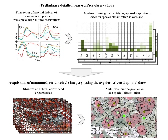
  • Phenology patterns are a key component in the discrimination of vegetation species, and near-surface sensors can be a reliable tool for obtaining a full annual time-series of individual plants.
  • The extraction of optimal dates for classification (when and how many) from a full near-surface time series can assist in optimizing the classification accuracy of sequential overhead data acquisition.
  • A large and representative sample of individuals reflects the variability within and between species, and is therefore essential for obtaining robust insights that can enable future implementation in similar areas.

1.3. Classification of East Mediterranean Vegetation by Remote Sensing

The typical East Mediterranean vegetation formations are dominated by multi-stemmed evergreen sclerophyllous trees or shrubs, summer semi-deciduous shrubs and a relatively small fraction of winter deciduous trees [47,48,49,50,51]. The extensive human influence in the region during the last thousands of years has led to a significant reduction in natural areas and to vast changes in species composition [52,53,54,55]. Therefore, accurate mapping of the local vulnerable high species richness is highly important for directing conservation efforts [56,57]. However, previous studies indicate that the East Mediterranean woody species are not necessarily an easy target for classification by remote sensing. Most local vegetation formations are characterized by densely-growing evergreen species, often with similar spectral properties [58,59,60], small intra-annual differences [61] and morphological similarities [62,63,64,65]. To the best of our knowledge, there are currently no studies that use high spatial resolution imagery with a limited number of bands for the classification of East Mediterranean common species.

2. Materials and Methods

2.1. Near-Surface Data Collection and Preprocessing

The following field work of remote sensing is described in detail in [61]. In brief, four sites, representing the Quercus calliprinos and Pistacia palaestina vegetation formation [47] were selected within the Judaean mountains in central Israel (Figure 1, see also Table 1 in [61]).
A modified Canon EOS 600D® camera was used for near-surface image acquisition of blue, green, red and near infra-red (NIR) bands [66,67,68] (Table 1). The data was collected for the duration of a full year, starting from 18 November 2015, weekly in the Sataf site (S′S facing south, and S′N facing north; [69]) or bi-weekly in the Mata and Britanya sites (M and B). On each date, a single image was acquired. The images were manually anchored to a single reference image, using between 20 to 50 points and the georeferencing Adjust function in ArcGIS 10.3® software (root mean square error = 0.27 pixels). Identification of species that could be recognized in the images was carried out in situ, resulting in 2704 individuals of 24 woody species and 93 patches of annual herbaceous vegetation (Supplementary Table S1). For each individual, an area-of-interest (AOI) polygon was digitized [70] within an illuminated part of the canopy [71]. Illumination correction was carried out by histogram shift, on the basis of fixed control AOIs [72]. Thereafter, the average values of nine spectral indices and three color conversions (red, green and blue, RGB; to hue, saturation and value, HSV) were computed within the species’ AOI, resulting in a tabular time series (Table 2). For the purpose of identifying the optimal dates for classification, the vegetation indices and color conversions were preferred over the original spectral bands, because they better express changes in vegetation condition, and because spectral band ratio indices are less sensitive than the original bands to shading effects (see references in Table 2).
With the exception of the annual minimum and maximum, local peaks in which the average difference between the previous and following dates exceeded ten percent of the annual range were defined as outliers. The outliers were replaced by the average of the two prior and two following dates. In addition, individuals with over 40% of outliers among the ExG (see Table 2) time series were not included in the following analysis (ExG was found to have a high signal to noise ratio; see [61]). The final dataset included 1852 individuals of 11 species and herbaceous patches. After the removal of outliers, a weighted scatterplot smoothing function (LOESS) was adjusted to all spectral indices time series [41,89].

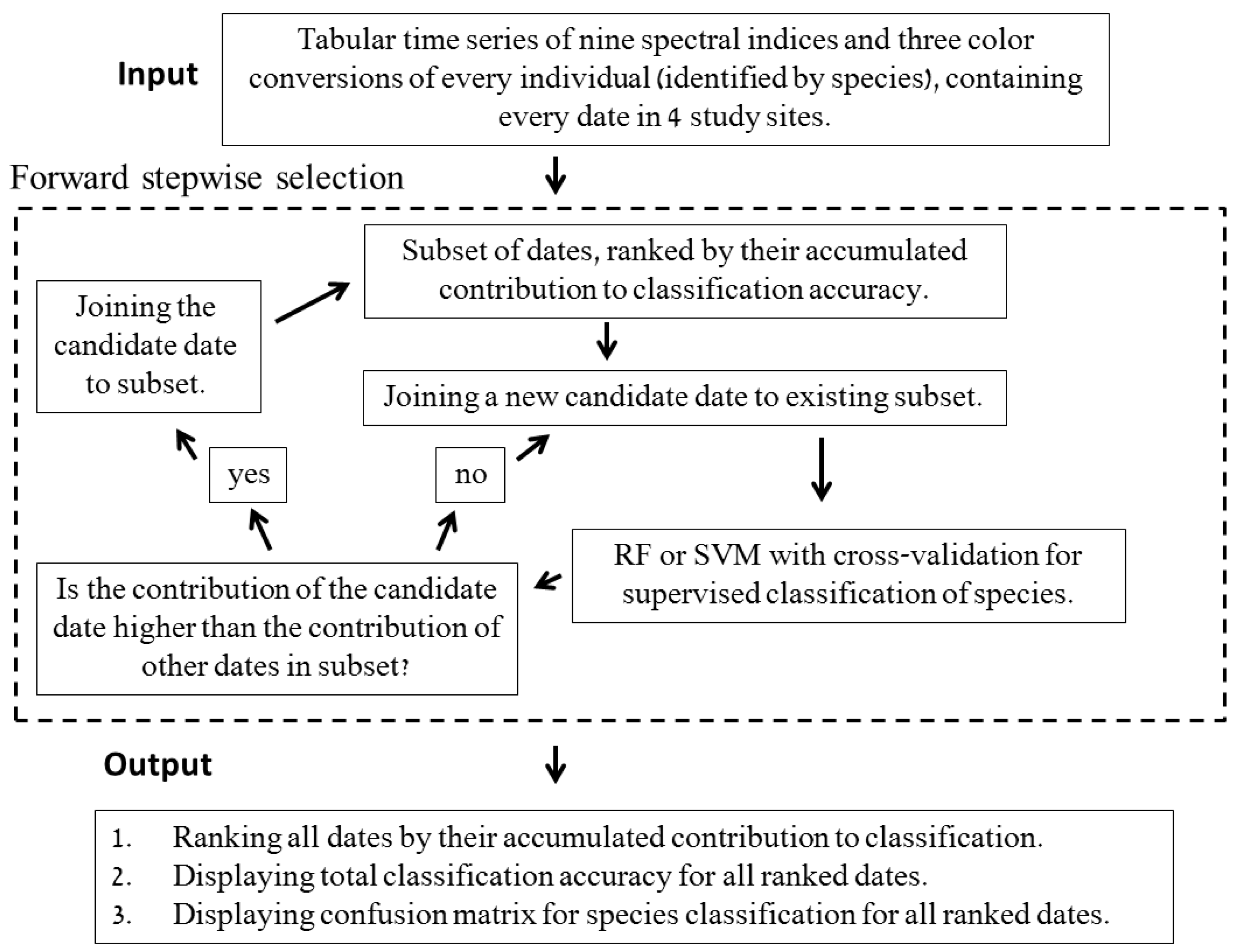
2.2. Selecting Optimal Acquisition Times for Species Classification on the Basis of the Near-Surface Time Series

The tabular time series of the near-surface observations was used for identifying the number and timing of optimal times for classification. For each site, a forward stepwise-selection of dates was conducted. The procedure used was as follows: the list of dates to be used was initialized as an empty list. At each step, the effect of adding each of the remaining unused dates to the list of dates to be used was tested using support vector machine (SVM) or random forest (RF) classifiers [90,91]. The date with the highest contribution was then added permanently to the list of dates to be used (so that after k steps the list contains exactly k dates). When applying a classifier on a list of dates, all spectral indices from the appropriate dates were used as features (Figure 2 and Supplementary S2). This analysis was computed using the Scikit-learn Python library [92].
Various features of the near–surface imagery time series classification process were examined in statistical tests (described below, 1–5). Due to optional variation in phenology between the sites, some of these aspects were examined only in the S′S site, which was selected because of the large sample of individuals from various species (Supplementary Table S1):
  • Comparison of the accumulated classification accuracy for the first ten optimal dates, using separate runs for testing the use of the RF and SVM classifier. We found that RF led to better classification accuracy compared to SVM, and therefore the following scenarios were all run using RF only (see Results). This was done using all spectral indices for observations in the S’S site only.
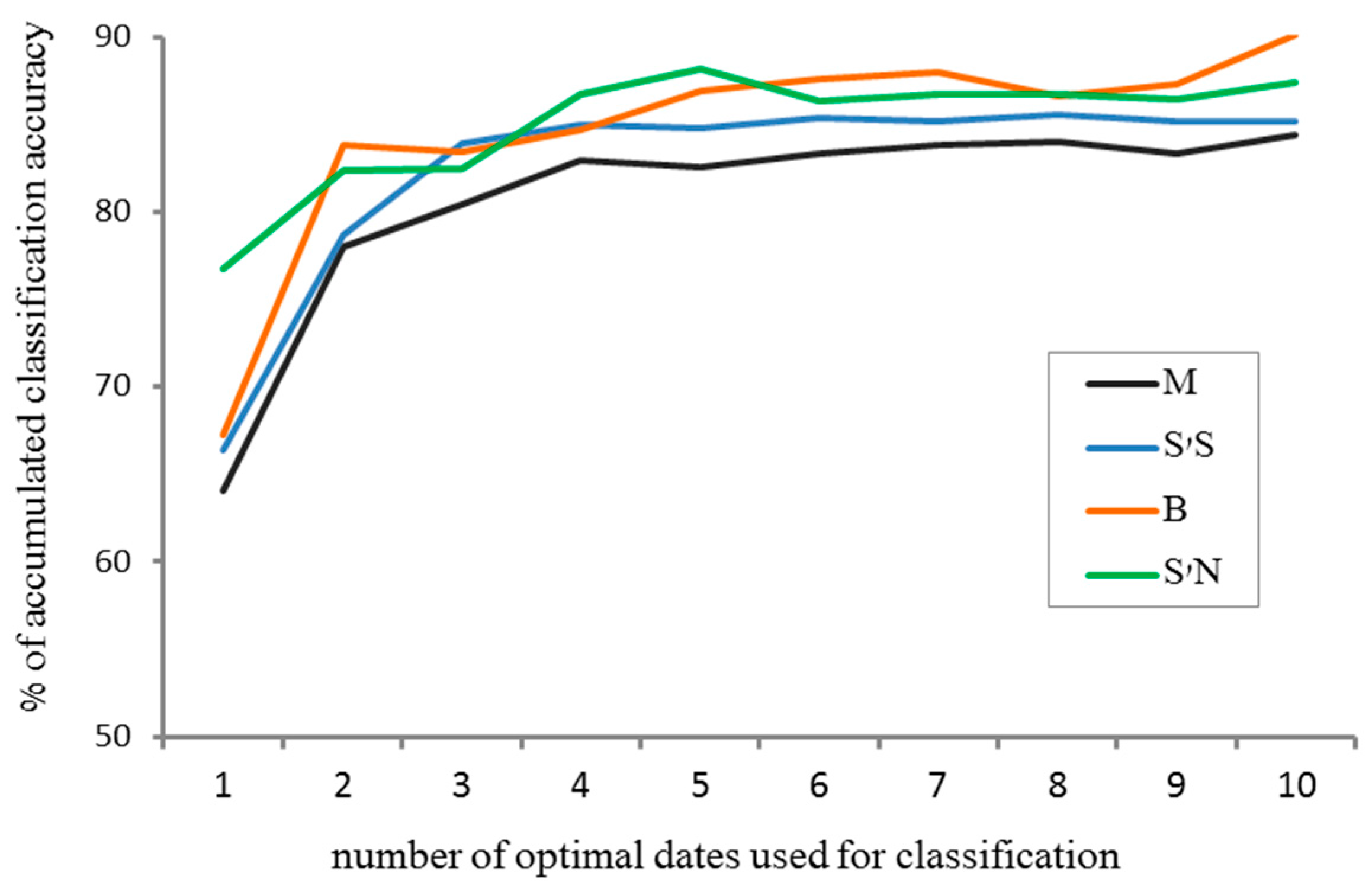
  • Comparison of the accumulated classification accuracy for the first ten optimal dates in all four sites, using RF, and all spectral indices were used as input.
  • Examining the accumulated classification accuracy for the first ten optimal dates, comparing between using different combinations of the spectral indices (see Results), in order to examine their contribution to classification accuracy. This was done by using RF, for observations in the S’S site only.
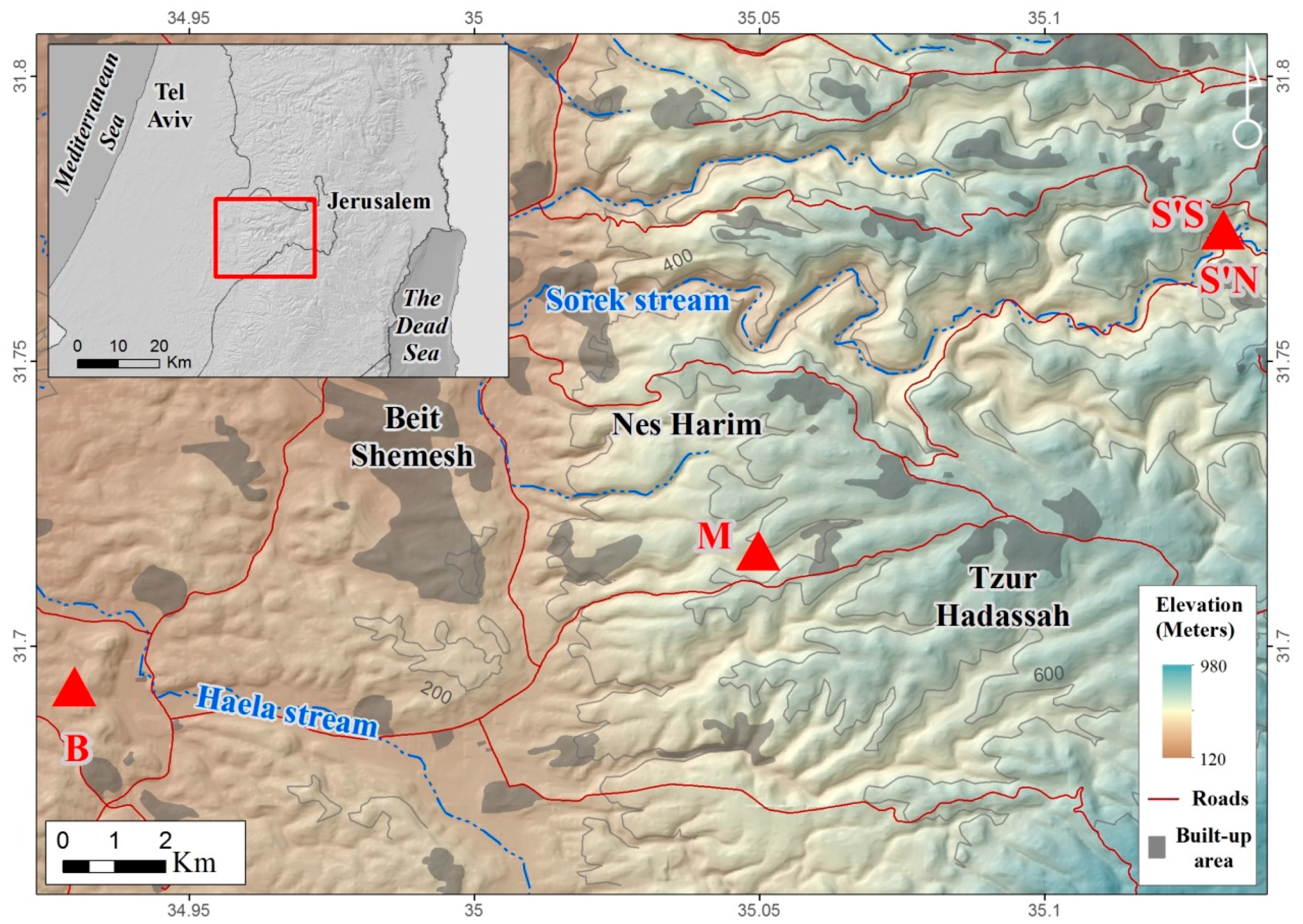
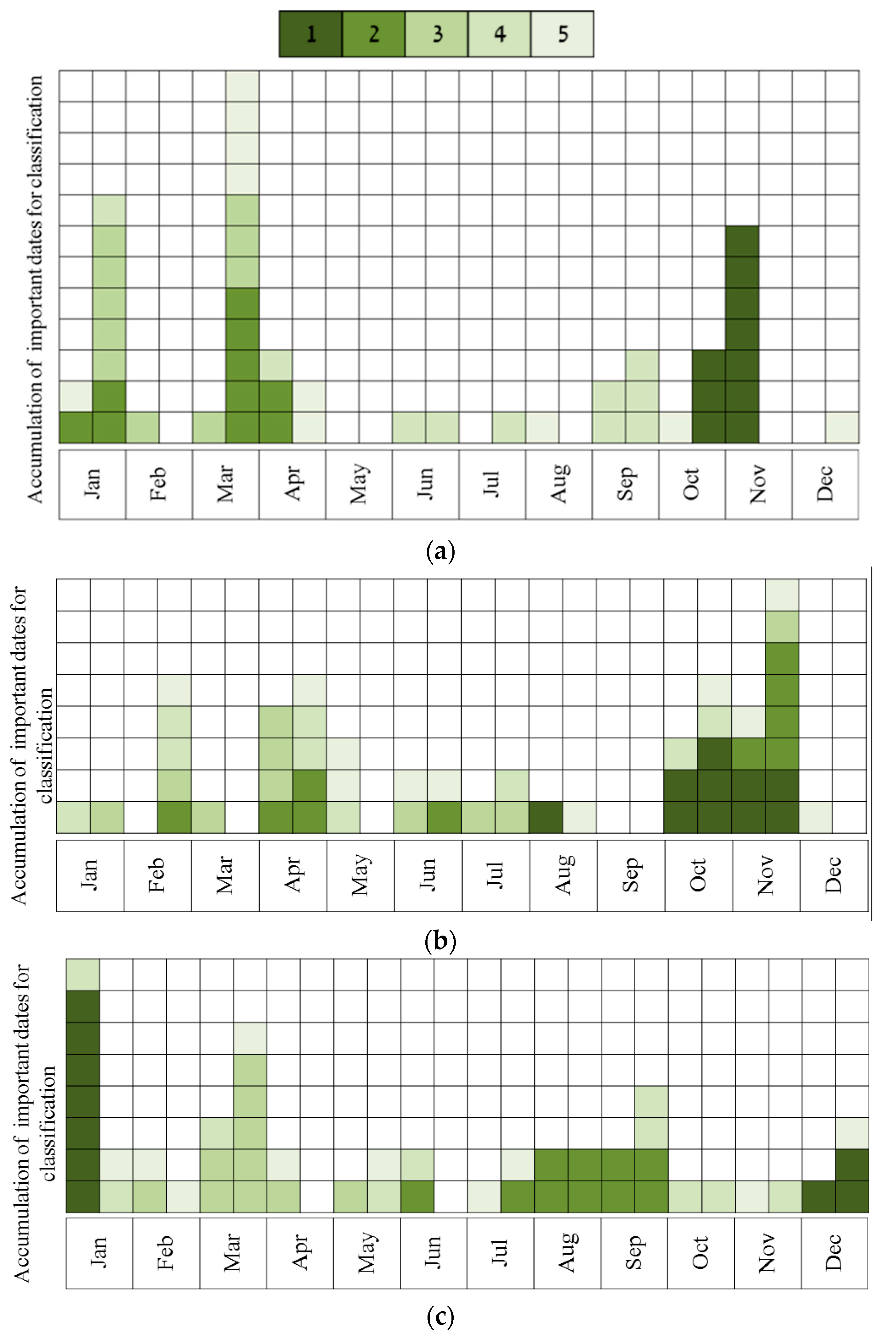
  • Describing the results of ten sequential runs—the most important five dates for classification of all species (the number of UAV acquisition times was set to five due to the findings of the above tests, see Results). This was carried out for all four sites. Ten sequential runs were used because of the need to evaluate the robustness of the results, since the classification process included random components (RF and the internal division of subsets for cross-validation). This was done by using RF, and all spectral indices as input.
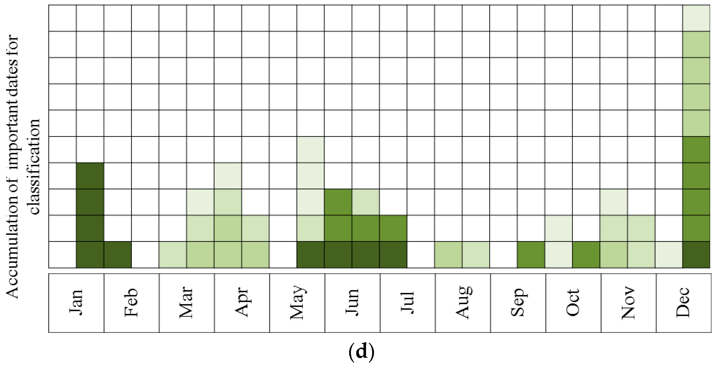
  • Describing the results of ten sequential runs—the most important five dates for discrimination between Pinus halepensis (evergreen conifer) and Quercus calliprinos (evergreen broad-leaved) in the S’S site. The classification was carried out by RF, using all spectral indices. The purpose of this scenario was to examine the proposed methodology for the discrimination of specific species. These species were selected because of the practical management need for mapping P. halepensis, which is a dominant factor in the occurrence of intensive forest fires in Israel, and which is additionally spreading from dense plantations to the surrounding natural vegetation, dominated by Q. calliprinos [93,94].

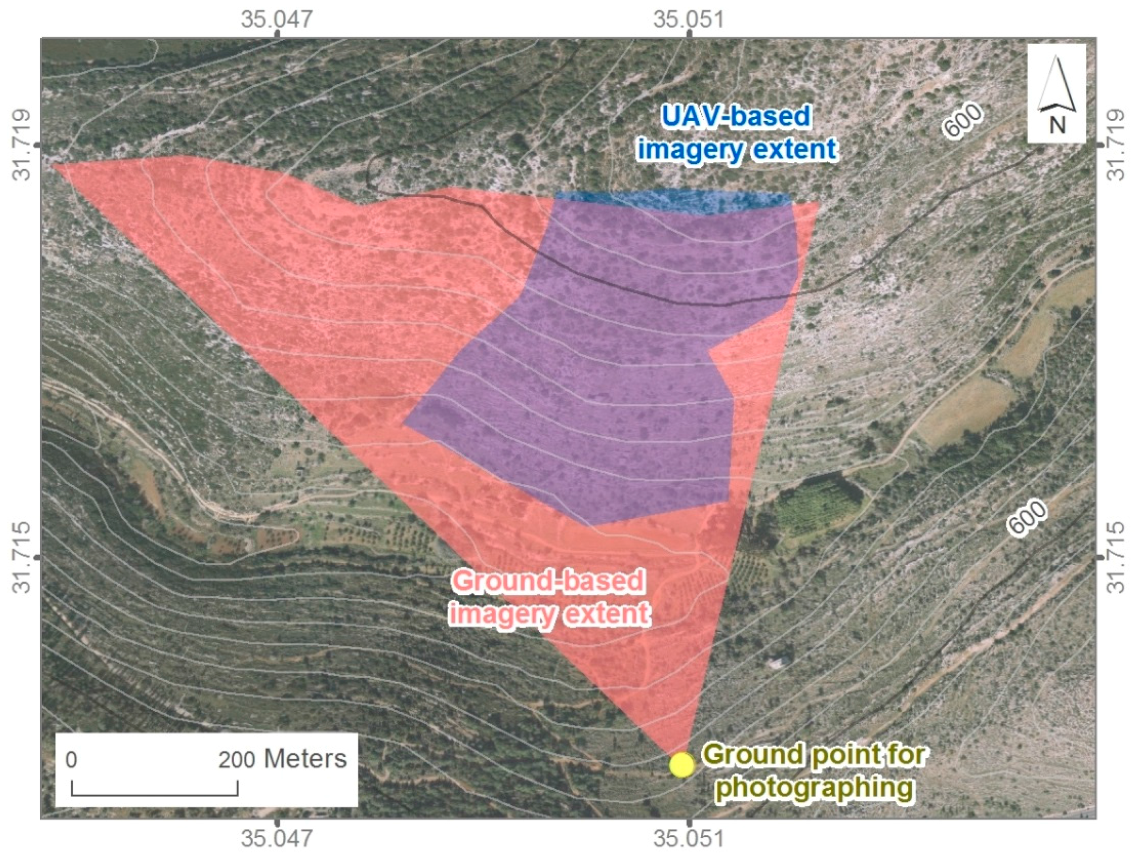
2.3. Overhead Data Acquisition and Species Classification

The Mata (M) site was chosen for the overhead-image classification because of a moderate topographic slope, a large number of individuals and a representative species composition (Supplementary Table S3). Following the research objectives, we used the results of the preliminary analysis of optimal periods for classification, as obtained from the near-surface time series (see results section). On the basis of a single run of the feature selection process, five periods for overhead data collection were specified for the M site (Table 3). The actual overhead data acquisition dates did not fit the exact optimal dates that were detected in the feature selection process, mainly because of the need for clear sky conditions as a requisition for quality imagery.
A Micasense Rededge® camera (https://www.micasense.com/rededge), designed for UAV platforms, was used for collecting overhead imagery (Table 1). The camera included five narrow-band separate sensors: blue (center ~490 nm, width 20 nm), green (center ~510 nm, width 20 nm), red (center ~670 nm, width 10 nm), red-edge (center ~720 nm, width 10 nm) and near infra-red (center ~840 nm, width 40 nm). Similar narrow-band sensors were found more suitable for vegetation sensing compared to regular consumer-grade cameras [95,96]. The camera produced 1.2 mega-pixel images in a 12-bit raw format. In addition to the five sensors that face downwards, the camera included a single sensor that was faced upwards and measured the real-time solar irradiation, as part of the preprocessing calibration. The camera was placed on a fixed-wing UAV, self-produced by Aeromap®.
Images were acquired at midday, in order to reduce the shading effects on the classification process. Following the manufacturer’s instructions, we used a reference board with known albedo values for the calibration of the camera before and after every flight. The spatial overlap between the adjacent images was predefined to 80% [97]. All in all, 340 separate images measuring on average 99 × 133 m on ground level were produced for each date. A 0.1 square kilometer five-band orthomosaic was produced, partly overlapping the extent of the ground-based images, using Micasense online processing services (Figure 3 and Figure 4a). The online processing included the structure from motion (SFM) procedure for creating the orthomosaic. The average orthomosaic pixel size on the ground was affected by changes in the distance between the fixed altitude of the UAV’s track and the ground (due to sloping topography), and was approximately 20 cm on average. The orthomosaics of all dates were manually anchored to the first image, using 50 points for each image and the georeferencing function in ArcGIS 10.3® software (root mean square error = 2.6 cm).
The multi-resolution segmentation algorithm in eCognition essentials 1.3® software was used for segmenting the UAV imagery [30,98,99,100,101,102]. The algorithm defines spatial differentiated polygonal objects on the basis of spatial and spectral homogeneities in the input image [103]. Since the timing of the phenophase with full foliage and canopy area varied between the deciduous species (e.g., winter deciduous trees and summer semi-deciduous shrubs), Normalized Difference Vegetation Index (NDVI) values (see Table 2) were calculated for all five dates, and we used their first principal component (containing 82% of original NDVI variance) as the input for segmentation (Figure 4b,c; [104]).
Average object size and shape characteristics of the multi-resolution segmentation can be supervised by defining a scale parameter; by the ratio between smoothness and compactness; and by the ratio between color and shape (constituting the leading factor during boundary determination). On the basis of visual examination of various trials, the scale parameter was set to three; the smoothness and compactness ratio was set to 0.6:0.4 (respectively); and the shape and color parameter ratio was set to 0.1:0.9 (respectively) [6,29,105].
Pixels with no contribution to the classification were removed, using two filters. The first filter removed shaded pixels [34], by omitting pixels with a red band value under five percent of the total range, for all five dates. The second filter removed pixels with no foliage, by omitting pixels with a maximal NDVI value (for all five dates) under 0.5 (Figure 4d).
Within the UAV imagery extent of the Mata site (M), the species of individual trees and shrubs were defined in a field survey. All in all, 1270 individuals of 16 species were mapped and digitized as a point GIS (Geographic Information Systems) layer, using ArcGIS 10.3® software. Cistus salviifolius and Cistus creticus were mapped as Cistus sp due to significant morphological similarities. One hundred and sixteen annual herbaceous patches were digitized by examining the imagery. In order to properly represent the foliage properties of the various species, we selected only segments that included an illuminated part of the canopy (after using the two filters), resulting in 976 segments (segments with inaccurate boundaries, e.g., including the canopy of more than one individual, were manually omitted, so as to ensure that each segment refers to a specific individual; Figure 4e and Supplementary Table S3). The ground-truth points were used in order to attribute to each selected segment its species affiliation as determined in the field survey. Species that were represented by less than 40 segments were not included in the following mapping process because of the need for a reasonable sample size, due to the following step of splitting the data to training and validation subsets (see below, resulting in a minimum of 20 individuals for each subset). Overall, the classified segments included nine woody species and additional annual herbaceous patches.
In order to perform a cross-validation of the classification process, the 976 segments were randomly divided to a subset for supervised classification training, and a separate subset for validation [35,97,106,107]. Each subset contained 50% of the segments, with an equal representation of species. The stratified random division was repeated ten times. In order to represent the spectral and phenological characteristics of the species, for every cross-validation run the combination of NDVI values from all dates, together with the first seven principle components (after using Principle Component Analysis, PCA) of visible bands from all dates, was used as the raster input. This combination was chosen after examining the overall classification accuracy of various inputs, including the red-edge band that was not represented in the chosen combination, because it did not improve the classification results. The segment classification was carried out by RF classifier, using eCognition software. Our overall approach of using near-surface observation for optimizing the use of following overhead data acquisition is summarized in Figure 5.

3. Results

3.1. Obtaining Optimal Dates for Species Classification from Near-Surface Observations

RF was more effective with regard to the first four optimal dates (classification accuracy of 80% for the second optimal date, compared to 64% with SVM, Figure 6). After the first few optimal dates (three for RF, five for SVM) there were no prominent improvements in the total classification accuracy of the near-surface time series (however, after the first seven optimal dates, SVM gained a small advantage in classification accuracy). Due to the aforementioned results, the following scenarios were run using RF as a single classifier.
The differences in classification accuracy between the four sites were small (Figure 7). The dissimilarities between sites could be related to the different species composition (see species composition in Supplementary Table S1 and confusion matrix, Supplementary Tables S4–S7).
The NIR band did not have a substantial contribution to the total classification accuracy of the near-surface time series. After the first two optimal dates, the total accuracy with no NIR-based spectral indices was close to the output accuracy of all spectral indices (81% and 82%, respectively; Figure 8, scenario 1 and 2). The negligible contribution of the NIR band could be related to the relatively low signal to noise ratio of the external filter method [70]. In fact, by using only the chromatic coordinates of the three visible bands (relative blue, green and red; scenario 5), the output classification accuracy after the first two optimal dates also reached 81%. The addition of HSV conversion, NDVI, gNDVI, ExG, GRVI, EmE (see Table 2) and total brightness resulted in higher accuracy for the first two optimal dates, as well as a small improvement from the third optimal date and onwards (scenarios 1, 2 and 6; Figure 8). Using only HSV conversion, or ExG alone, resulted in lower classification accuracy (70% and 72% for the third optimal date, respectively; scenarios 3 and 4; Figure 8).
The scattering of the optimal dates for classification of the near-surface time series throughout the year differed between the four sites, and in all cases was not distributed evenly over time (Figure 9a–d). However, the first optimal period for classification occurred during the late fall (November–December; S′S, S′N) or early winter (December–January; M), with the exception of site B (divided between winter, December–February, and summer, May–July). Nevertheless, despite the lack of consistency among sequential runs in the same site, the classification accuracy remained stable; the average standard deviation of overall accuracy in the four sites after the five optimal dates was 0.83%.
Thus, in each site, the feature selection process identified various combinations of optimal dates, resulting in similar classification accuracy. Therefore, the identified optimal dates of a single run output were not necessarily the absolute single solution; however they could be used for planning sequential data acquisition dates regarding phenology-based classification. As mentioned above, the difference in the combination of optimal dates between sites was probably related to the dissimilarities in species composition.
P. halepensis and Q. calliprinos are both evergreen, and they do not demonstrate prominent visual differences throughout the year. However, Figure 10 demonstrates the convergence of all cross-validation runs, pointing at the second half of April (end of spring) as the most important period for separation between the two species. This consistently selected period matches the flowering and leaves growth of Q. calliprinos [61,108]. Apparently the spectral expression of this phenophase results in improved ability of discrimination from P. halepensis, since after the five most important dates for classification the average overall accuracy of the 10 sequential runs was 98%.

3.2. Overhead Data Acquisition and Species Classification

The overhead time series imagery demonstrates visually the discrimination between the main phenological groups (Figure 11). Rocks, trails and ruins appear in black because of low and fixed NDVI values. Herbaceous patches and partial summer deciduous shrubs appear in shades of green because of the prominent NDVI peak during spring. Winter deciduous trees appear in shades of blue because the foliage cover is developed during late spring, and the NDVI values are relatively high and stable during early summer. Evergreen trees and shrubs appear in bright colors due to high NDVI values all year round. The UAV derived NDVI values of the evergreen species and the herbaceous patches both presented a similar annual pattern to those acquired by the preliminary near-surface observations, despite the different range of values resulting from the significant differences between the sensors (Figure 12). The NDVI values of the deciduous species in the first UAV image (20 December 2016) were lower than those of the parallel near-surface values, possibly due to the exceptional absence of autumn precipitation during the fall of 2016 (Figure 13).
The ten cross-validation accuracy assessments of the UAV time series classification resulted in an average overall accuracy of 85% and an average Kappa coefficient of 0.82 (Table 5). Average producer’s accuracy ranged between 94.2% (herbaceous patches) and 76.9% (Olea europaea). Average user’s accuracy ranged between 97.1% (herbaceous patches) and 64.6% (Olea europaea). The average producer’s and user’s accuracy values of the different species were not necessarily assigned to phenological groups (e.g., evergreen vs. deciduous). However, the unique green phenophase of herbaceous patches during the limited period of the wet season [109] led to a high classification accuracy compared to the woody species.

4. Discussion

4.1. Species-Driven Approach as a Key Component for Applicative Species Mapping by Remote Sensing

As opposed to data-driven studies that focus on maximizing classification accuracy within a limited framework, and therefore are of limited value for implementation [1], in this study we present a species-driven approach, focusing on the temporal traits that affect the classification success. An essential component of the presented methodology is the large assembly of individuals used for obtaining detailed phenology observations, as well as for examining the feasibility of individual classification to species. We examined four different sites of different environmental conditions, containing a large number of species that included the common components of the local vegetation formations. Each species was represented by a large number of individuals, including the within-species morphological and phenological heterogeneity. The large representative sample improves the ability of using the research outcomes regarding applied mapping of the same species in similar East Mediterranean habitats. By using the feature selection process, various objectives can be examined on the basis of the existing near-surface dataset. Relevant objectives in similar sites could be the optimization of overall classification for all species, discrimination between two target species, or discrimination of one invasive species from all local species.
We did not choose to focus on ideal target species (e.g., large homogeneous canopies with visually distinct phenophases), rather, we examined the local species assembly as-is, including species with challenging spectral and morphological properties with regard to classification by remote sensing [59,60,62,65]; furthermore, after examining the preliminary classification results, we did not see fit to merge or omit species in order to increase overall accuracy.
Nonetheless, in addition to the abovementioned phenological heterogeneity within and between species and the influence of different environmental conditions [110,111,112], intra-annual variability is also an important factor [74,113]. Since the presented methodology uses insights that are obtained from near-surface observations of a single phenological cycle for determining optimal periods during the sequential phenological cycles, intra-annual variability could affect the robustness of the presented outcomes. Further research should relate to this issue, inter alia by displaying the intra-annual consistency of optimal periods throughout several years, or by presenting a prediction model based on climatic characteristics of a specific year. In the context of applied mapping, the ability to focus on specific species (as in the presented case study of discriminating between P. halepensis and Q. calliprinos) can assist in adapting the optimal period for classification to intra-annual phenological variability, by defining the important phenophases of the relevant species and identifying their occurrence in the field.
It should be noted that the presented methodology used for classifying the overhead imagery involved manual selection of appropriate segments for training and validation. In the context of implementing the above-mentioned method over larger areas, this step should necessarily be replaced by an automated method of segment selection, e.g., texture and shape analysis.

4.2. Near-Surface Phenological Observations and Sequential UAV Repetitive Imagery as a Cost-Effective Methodology for Detailed Vegetation Mapping

As mentioned above, due to the similarity between the spectral signatures of vegetation species [114,115], high quality hyperspectral imagery and optional LiDAR is usually required in order to properly discriminate between species on the basis of remote sensing [10,13,116,117]. In the case of individual-level vegetation mapping, these inputs should be of very high spatial resolution. Despite the proven success of this approach [8], it is unlikely to be widely adopted in the near future by practitioners in governmental or non-governmental organizations for applied mapping at a regional scale. This is first of all because of the high costs that are involved in producing appropriate cutting-edge imagery from airborne hyperspectral sensors over large areas and the present lack of spaceborne hyperspectral sensors with a high signal to noise ratio, but also due to technical considerations such as storage and processing limitations [1]. Nevertheless, the presented methodology of using a priori near-surface insights could be used also for optimizing the temporal use of hyper-spectral or LiDAR sensors.
Maximizing the contribution of prominent phenophases to species discrimination using basic spectral information can also substitute cutting edge hyperspectral approaches for evergreen species [39]. Obtaining preliminary spectral and phenological information for optimizing sequential repetitive imagery acquisition using UAVs can provide organizations that administrate natural areas an effective applicable tool for high-quality vegetation mapping. In the context of cost-effectiveness [1], the presented methodology can be easily implemented within a reasonable overall cost by using accessible off-the-shelf products. For obtaining preliminary phenological information, a consumer-grade digital camera with no NIR capabilities is sufficient (see Figure 8) [61,70,118,119]; drones and other available fixed wing UAVs have been proven to be a suitable tool for collecting repetitive high-quality overhead imagery [6,34,35,120]; while open source free GIS software’s (Geographic Information Systems; e.g., QGIS and R) includ sufficient image processing tools.

4.3. Relevant Implications for Satellite Imagery

It should be noted that a significant limitation of UAV-based mapping is the relatively limited survey area. In addition to the use of UAVs for individual identification of vegetation species, current advances in satellite platforms can make the presented methodology applicable over larger areas. High spatial resolution satellite-based imagery is currently available with a high revisit time (e.g., nano-satellites such as Planet® imagery; [120,121,122,123]) and will be even more accessible in the near future (e.g., the DigitalGlobe® Scout program or the Venµs project [124]). The temporal resolution of these satellites is apparently sufficient for focusing on pre-defined phenophases (e.g., a two-day revisit time for the Venµs project). However, the spatial resolution is still a notable limitation compared to UAV imagery (5.3 m for Venµs, three meters for Planet® nano-satellites), since the discrimination of individual species requires the use of pixels that are significantly smaller than the individual level. This limitation is obligatory for the Mediterranean species that were examined in the current study, and is especially significant when using segmentation as part of the classification process. Yet, the use of near-surface observations for optimizing the above-mentioned satellite imagery can be used for classifying habitats with monocultural vegetation patches, communities with a dominant species, or single trees with large canopies [32,33]. Under these limitations, a notable advantage of using satellite imagery compared to UAV imagery is the expanded mapping area.

5. Conclusions

The use of preliminary detailed near-surface observations for optimizing the timing of high resolution image acquisition resulted in high accuracy identification of a representative assemblage of local woody vegetation species, despite spectral and phenological similarities. This approach focused on the phenological properties of the target species, and can be applied to the same species in other sites. The methodology included cost-effective and accessible data collection tools, which can be used by practitioners for applied detailed mapping of vegetation, as opposed to cutting edge hyperspectral sensors. Future research should refer to the effect of intra-annual variance on the robustness of the optimized timing for image acquisition.

Supplementary Materials

The following are available online at www.mdpi.com/2072-4292/9/11/1130/s1, Table S1: Number of individuals for each species, regarding the near-surface time series analysis; S2: Technical description of the forward stepwise-selection process; Table S3: Number of individuals for each species, regarding the overhead imagery analysis in site Mata (M); Table S4: Confusion matrix for the classification results of the Sataf south-facing site (S’S), using the five optimal dates. The classification was carried out by RF classifier, using all spectral indices; Table S5: Confusion matrix for the classification results of the Sataf north-facing site (S’N), using the five optimal dates. The classification was carried out by RF classifier, using all spectral indices; Table S6: Confusion matrix for the classification results of the Mata site (M), using the five optimal dates. The classification was carried out by RF classifier, using all spectral indices; Table S7: Confusion matrix for the classification results of the Britanya site (B), using the five optimal dates. The classification was carried out by RF classifier, using all spectral indices.

Acknowledgments

We would like to thank the Ring Family Foundation for Atmospheric and Global Studies and the Amiran Fund from the Hebrew University of Jerusalem for their support, as well as the Israel Nature and Parks Authority for their backing of this research. We are grateful to Ami Wiesel for his helpful advice.

Author Contributions

Noam Levin and Itamar M. Lensky supervised the research; Gilad Weil performed the near-surface observations, the in-situ surveys, characterized the feature selection process, analyzed the data and wrote the paper; Yehezkel S. Resheff wrote the feature selection code.

Conflicts of Interest

The authors declare no conflict of interest.

References

  1. Fassnacht, F.E.; Latifi, H.; Stereńczak, K.; Modzelewska, A.; Lefsky, M.; Waser, L.T.; Ghosh, A. Review of studies on tree species classification from remotely sensed data. Remote Sens. Environ. 2016, 186, 64–87. [Google Scholar] [CrossRef]
  2. Kerr, J.T.; Ostrovsky, M. From space to species: Ecological applications for remote sensing. Trends Ecol. Evol. 2003, 18, 299–305. [Google Scholar] [CrossRef]
  3. Mulla, D.J. Twenty five years of remote sensing in precision agriculture: Key advances and remaining knowledge gaps. Biosyst. Eng. 2003, 114, 358–371. [Google Scholar] [CrossRef]
  4. Rocchini, D.; Boyd, D.S.; Féret, J.B.; Foody, G.M.; He, K.S.; Lausch, A.; Pettorelli, N. Satellite remote sensing to monitor species diversity: Potential and pitfalls. Remote Sens. Ecol. Conserv. 2015, 2, 25–36. [Google Scholar] [CrossRef]
  5. Vilà, M.; Vayreda, J.; Comas, L.; Ibáñez, J.J.; Mata, T.; Obón, B. Species richness and wood production: A positive association in Mediterranean forests. Ecol. Lett. 2007, 10, 241–250. [Google Scholar] [CrossRef] [PubMed]
  6. Müllerová, J.; Bruna, J.; Dvorák, P.; Bartalos, T.; Vítková, M. Does the Data Resolution/origin Matter? Satellite, Airborne and UAV Imagery to Tackle Plant Invasions. Int. Arch. Photogram. Remote Sens. Spat. Inf. Sci. 2016, 41, 903–908. [Google Scholar] [CrossRef]
  7. Roth, K.L.; Roberts, D.A.; Dennison, P.E.; Peterson, S.H.; Alonzo, M. The impact of spatial resolution on the classification of plant species and functional types within imaging spectrometer data. Remote Sens. Environ. 2015, 171, 45–57. [Google Scholar] [CrossRef]
  8. Xie, Y.; Sha, Z.; Yu, M. Remote sensing imagery in vegetation mapping: A review. J. Plant Ecol. 2008, 1, 9–23. [Google Scholar] [CrossRef]
  9. Ferreira, M.P.; Zortea, M.; Zanotta, D.C.; Shimabukuro, Y.E.; de Souza Filho, C.R. Mapping tree species in tropical seasonal semi-deciduous forests with hyperspectral and multispectral data. Remote Sens. Environ. 2016, 179, 66–78. [Google Scholar] [CrossRef]
  10. Lawrence, R.L.; Wood, S.D.; Sheley, R.L. Mapping invasive plants using hyperspectral imagery and Breiman Cutler classifications (RandomForest). Remote Sens. Environ. 2006, 100, 356–362. [Google Scholar] [CrossRef]
  11. Paz-Kagan, T.; Caras, T.; Herrmann, I.; Shachak, M.; Karnieli, A. Multiscale Mapping of Species Diversity under Changed Land-Use Using Imaging Spectroscopy. Ecol. Appl. 2017. [Google Scholar] [CrossRef] [PubMed]
  12. Asner, G.P.; Martin, R.E. Airborne spectranomics: Mapping canopy chemical and taxonomic diversity in tropical forests. Front. Ecol. Environ. 2008, 7, 269–276. [Google Scholar] [CrossRef]
  13. Dalponte, M.; Bruzzone, L.; Gianelle, D. Fusion of hyperspectral and LIDAR remote sensing data for classification of complex forest areas. IEEE Trans. Geosci. Remote Sens. 2008, 46, 1416–1427. [Google Scholar] [CrossRef]
  14. Kozhoridze, G.; Orlovsky, N.; Orlovsky, L.; Blumberg, D.G.; Golan-Goldhirsh, A. Remote sensing models of structure-related biochemicals and pigments for classification of trees. Remote Sens. Environ. 2016, 186, 184–195. [Google Scholar] [CrossRef]
  15. Galidaki, G.; Gitas, I. Mediterranean forest species mapping using classification of Hyperion imagery. Geocarto Int. 2015, 30, 48–61. [Google Scholar] [CrossRef]
  16. Lieth, H. Phenology in productivity studies. In Analysis of Temperate Forest Ecosystems; Springer: Berlin/Heidelberg, Germany, 1973; pp. 29–46. [Google Scholar]
  17. Morisette, J.T.; Richardson, A.D.; Knapp, A.K.; Fisher, J.I.; Graham, E.A.; Abatzoglou, J.; Wilson, B.; Breshears, D.; Henebry, G.; Hanes, J.; et al. Tracking the rhythm of the seasons in the face of global change: Phenological research in the 21st century. Front. Ecol. Environ. 2009, 7, 253–260. [Google Scholar] [CrossRef]
  18. Rathcke, B.; Lacey, E.P. Phenological patterns of terrestrial plants. Annu. Rev. Ecol. Evol. 1985, 16, 179–214. [Google Scholar] [CrossRef]
  19. Dudley, K.L.; Dennison, P.E.; Roth, K.L.; Roberts, D.A.; Coates, A.R. A multi-temporal spectral library approach for mapping vegetation species across spatial and temporal phenological gradients. Remote Sens. Environ. 2015, 167, 121–134. [Google Scholar] [CrossRef]
  20. Hill, R.A.; Wilson, A.K.; George, M.; Hinsley, S.A. Mapping tree species in temperate deciduous woodland using time-series multi-spectral data. Appl. Veg. Sci. 2010, 13, 86–99. [Google Scholar] [CrossRef]
  21. Key, T.; Warner, T.A.; McGraw, J.B.; Fajvan, M.A. A comparison of multispectral and multitemporal information in high spatial resolution imagery for classification of individual tree species in a temperate hardwood forest. Remote Sens. Environ. 2001, 75, 100–112. [Google Scholar] [CrossRef]
  22. Madonsela, S.; Cho, M.A.; Mathieu, R.; Mutanga, O.; Ramoelo, A.; Kaszta, Ż.; Wolff, E. Multi-phenology WorldView-2 imagery improves remote sensing of savannah tree species. Int. J. Appl. Earth Obs. Geoinf. 2017, 58, 65–73. [Google Scholar] [CrossRef]
  23. Somers, B.; Asner, G.P. Multi-temporal hyperspectral mixture analysis and feature selection for invasive species mapping in rainforests. Remote Sens. Environ. 2013, 136, 14–27. [Google Scholar] [CrossRef]
  24. Anderson, K.; Gaston, K.J. Lightweight unmanned aerial vehicles will revolutionize spatial ecology. Front. Ecol. Environ. 2013, 11, 138–146. [Google Scholar] [CrossRef]
  25. Kaneko, K.; Nohara, S. Review of effective vegetation mapping using the UAV (Unmanned Aerial Vehicle) method. IJGIS 2014, 6, 733. [Google Scholar] [CrossRef]
  26. Pajares, G. Overview and current status of remote sensing applications based on unmanned aerial vehicles (UAVs). Photogramm. Eng. Remote Sens. 2015, 81, 281–329. [Google Scholar] [CrossRef]
  27. Watts, A.C.; Ambrosia, V.G.; Hinkley, E.A. Unmanned aircraft systems in remote sensing and scientific research: Classification and considerations of use. Remote Sens. 2012, 4, 1671–1692. [Google Scholar] [CrossRef]
  28. Crebassol, P.; Ferrier, P.; Dedieu, G.; Hagolle, O.; Fougnie, B.; Tinto, F.; Yaniv, Y.; Herscovitz, J. VENµS (Vegetation and Environment Monitoring on a New Micro Satellite). In Small Satellite Missions for Earth Observation; Springer: Berlin, Germany, 2010; pp. 47–65. [Google Scholar]
  29. Laliberte, A.S.; Goforth, M.A.; Steele, C.M.; Rango, A. Multispectral remote sensing from unmanned aircraft: Image processing workflows and applications for rangeland environments. Remote Sens. 2011, 3, 2529–2551. [Google Scholar] [CrossRef]
  30. Blaschke, T.; Johansen, K.; Tiede, D. Object-Based Image Analysis for Vegetation Mapping and Monitoring. In Advances in Environmental Remote Sensing: Sensor, Algorithms, and Applications; CRC Press: Boca Raton, FL, USA, 2011; pp. 241–271. [Google Scholar]
  31. Haralick, R.M.; Shanmugam, K. Textural features for image classification. IEEE Trans. Syst. Man Cybern. 1973, 3, 610–621. [Google Scholar] [CrossRef]
  32. Schmidt, T.; Schuster, C.; Kleinschmit, B.; Forster, M. Evaluating an Intra-Annual Time Series for Grassland Classification—How Many Acquisitions and What Seasonal Origin Are Optimal? IEEE J. STARS 2014, 7, 3428–3439. [Google Scholar] [CrossRef]
  33. Schuster, C.; Schmidt, T.; Conrad, C.; Kleinschmit, B.; Förster, M. Grassland habitat mapping by intra-annual time series analysis–Comparison of RapidEye and TerraSAR-X satellite data. Int. J. Appl. Earth Obs. Geoinf. 2015, 34, 25–34. [Google Scholar] [CrossRef]
  34. Lisein, J.; Michez, A.; Claessens, H.; Lejeune, P. Discrimination of deciduous tree species from time series of unmanned aerial system imagery. PLoS ONE 2015, 10, e0141006. [Google Scholar] [CrossRef] [PubMed] [Green Version]
  35. Michez, A.; Piégay, H.; Lisein, J.; Claessens, H.; Lejeune, P. Classification of riparian forest species and health condition using multi-temporal and hyperspatial imagery from unmanned aerial system. Environ. Monit. Assess. 2016, 188, 1–19. [Google Scholar] [CrossRef] [PubMed]
  36. Cole, B.; McMorrow, J.; Evans, M. Spectral monitoring of moorland plant phenology to identify a temporal window for hyperspectral remote sensing of peatland. ISPRS J. Photogramm. Remote Sens. 2014, 90, 49–58. [Google Scholar] [CrossRef]
  37. Feilhauer, H.; Thonfeld, F.; Faude, U.; He, K.S.; Rocchini, D.; Schmidtlein, S. Assessing floristic composition with multispectral sensors—A comparison based on monotemporal and multiseasonal field spectra. Int. J. Appl. Earth Obs. Geoinf. 2013, 21, 218–229. [Google Scholar] [CrossRef]
  38. Féret, J.B.; Corbane, C.; Alleaume, S. Detecting the phenology and discriminating Mediterranean natural habitats with multispectral sensors—An analysis based on multiseasonal field spectra. IEEE J. STARS 2015, 8, 2294–2305. [Google Scholar] [CrossRef]
  39. Van Deventer, H.; Cho, M.A.; Mutanga, O. Improving the classification of six evergreen subtropical tree species with multi-season data from leaf spectra simulated to WorldView-2 and RapidEye. Int. J. Remote Sens. 2017, 38, 4804–4830. [Google Scholar] [CrossRef]
  40. Richardson, A.D.; Jenkins, J.P.; Braswell, B.H.; Hollinger, D.Y.; Ollinger, S.V.; Smith, M.L. Use of digital webcam images to track spring green-up in a deciduous broadleaf forest. Oecologia 2007, 152, 323–334. [Google Scholar] [CrossRef] [PubMed]
  41. Sonnentag, O.; Hufkens, K.; Teshera-Sterne, C.; Young, A.M.; Friedl, M.; Braswell, B.H.; Richardson, A.D. Digital repeat photography for phenological research in forest ecosystems. Agric. For. Meteorol. 2012, 152, 159–177. [Google Scholar] [CrossRef]
  42. Wingate, L.; Ogée, J.; Cremonese, E.; Filippa, G.; Mizunuma, T.; Migliavacca, M.; Grace, J. Interpreting canopy development and physiology using a European phenology camera network at flux sites. Biogeosciences 2015, 12, 5995–6015. [Google Scholar] [CrossRef] [Green Version]
  43. Almeida, J.; dos Santos, J.A.; Alberton, B.; Morellato, L.P.C.; Torres, R.D.S. Phenological visual rhythms: Compact representations for fine-grained plant species identification. Pattern Recognit. Lett. 2016, 81, 90–100. [Google Scholar] [CrossRef]
  44. Ide, R.; Oguma, H. Use of digital cameras for phenological observations. Ecol. Inform. 2010, 5, 339–347. [Google Scholar] [CrossRef]
  45. Bater, C.W.; Coops, N.C.; Wulder, M.A.; Hilker, T.; Nielsen, S.E.; McDermid, G.; Stenhouse, G.B. Using digital time-lapse cameras to monitor species-specific understorey and overstorey phenology in support of wildlife habitat assessment. Environ. Monit. Assess. 2011, 180, 1–13. [Google Scholar] [CrossRef] [PubMed]
  46. Snyder, K.A.; Wehan, B.L.; Filippa, G.; Huntington, J.L.; Stringham, T.K.; Snyder, D.K. Extracting Plant Phenology Metrics in a Great Basin Watershed: Methods and Considerations for Quantifying Phenophases in a Cold Desert. Sensors 2016, 16, 1948. [Google Scholar] [CrossRef] [PubMed]
  47. Danin, A. Flora and vegetation of Israel and adjacent areas. In The Zoogeography of Israel; Dr. W. Junk Publishers: Dordrecht, The Netherlands, 1988; pp. 251–276. [Google Scholar]
  48. Shmida, A. Mediterranean vegetation in California and Israel: Similarities and differences. Isr. J. Bot. 1981, 30, 105–123. [Google Scholar]
  49. Miller, P.C. Canopy structure of Mediterranean-type shrubs in relation to heat and moisture. In Mediterranean-Type Ecosystems; Springer: Berlin/Heidelberg, Germany, 1983; pp. 133–166. [Google Scholar]
  50. Ne’eman, G.; Goubitz, S. Phenology of east Mediterranean vegetation. In Life and Environment in the Mediterranean; WIT Press: Ashurst, UK, 2000; pp. 155–201. [Google Scholar]
  51. Orshan, G. Approaches to the definition of Mediterranean growth forms. In Mediterranean-Type Ecosystems; Springer: Berlin/Heidelberg, Germany, 1983; pp. 86–100. [Google Scholar]
  52. Kadmon, R.; Harari-Kremer, R. Studying long-term vegetation dynamics using digital processing of historical aerial photographs. Remote Sens. Environ. 1999, 68, 164–176. [Google Scholar] [CrossRef]
  53. Levin, N. Human factors explain the majority of MODIS-derived trends in vegetation cover in Israel: A densely populated country in the eastern Mediterranean. Reg. Environ. Chang. 2016, 16, 1197–1211. [Google Scholar] [CrossRef]
  54. Naveh, Z. Mediterranean landscape evolution and degradation as multivariate biofunctions: Theoretical and practical implications. Landsc. Plan 1982, 9, 125–146. [Google Scholar] [CrossRef]
  55. Perevolotsky, A.; Seligman, N.A.G. Role of grazing in Mediterranean rangeland ecosystems. Bioscience 1998, 48, 1007–1017. [Google Scholar] [CrossRef]
  56. Mandelik, Y.; Roll, U.; Fleischer, A. Cost-efficiency of biodiversity indicators for Mediterranean ecosystems and the effects of socio-economic factors. J. Appl. Ecol. 2010, 47, 1179–1188. [Google Scholar] [CrossRef]
  57. Radford, E.A.; Catullo, G.; de Montmollin, B. Important plant areas of the south and east Mediterranean region: Priority sites for conservation. International Union for Conservation of Nature, Plantlife, WWF, 2011. Available online: https://portals.iucn.org/library/sites/library/files/documents/2011-014.pdf (accessed on 17 September 2017).
  58. Manakos, I.; Manevski, K.; Petropoulos, G.P.; Elhag, M.; Kalaitzidis, C. Development of a spectral library for Mediterranean land cover types. In Proceedings of the 30th EARSeL Symposium: Remote Sensing for Science, Education and Natural and Cultural Heritage, Paris, France, 31 May–4 June 2010. [Google Scholar]
  59. Manevski, K.; Manakos, I.; Petropoulos, G.P.; Kalaitzidis, C. Discrimination of common Mediterranean plant species using field spectroradiometry. Int. J. Appl. Earth Obs. Geoinf. 2011, 13, 922–933. [Google Scholar] [CrossRef]
  60. Rud, R.; Shoshany, M.; Alchanatis, V.; Cohen, Y. Application of spectral features’ ratios for improving classification in partially calibrated hyperspectral imagery: A case study of separating Mediterranean vegetation species. J. Real Time Image Process. 2006, 1, 143–152. [Google Scholar] [CrossRef]
  61. Weil, G.; Lensky, I.M.; Levin, N. Using ground observations of a digital camera in the VIS-NIR range for quantifying the phenology of Mediterranean woody species. Int. J. Appl. Earth Obs. Geoinf. 2017, 62, 88–101. [Google Scholar] [CrossRef]
  62. Bar Massada, A.; Kent, R.; Blank, L.; Perevolotsky, A.; Hadar, L.; Carmel, Y. Automated segmentation of vegetation structure units in a Mediterranean landscape. Int. J. Remote Sens. 2012, 33, 346–364. [Google Scholar] [CrossRef]
  63. Bashan, D.; Bar-Massada, A. Regeneration dynamics of woody vegetation in a Mediterranean landscape under different disturbance-based management treatments. Appl. Veg. Sci. 2017, 20, 106–114. [Google Scholar] [CrossRef]
  64. Carmel, Y.; Kadmon, R. Computerized classification of Mediterranean vegetation using panchromatic aerial photographs. J. Veg. Sci. 1998, 9, 445–454. [Google Scholar] [CrossRef]
  65. Shoshany, M. Satellite remote sensing of natural Mediterranean vegetation: A review within an ecological context. Prog. Phys. Geogr. 2000, 24, 153–178. [Google Scholar] [CrossRef]
  66. Džubáková, K.; Molnar, P.; Schindler, K.; Trizna, M. Monitoring of riparian vegetation response to flood disturbances using terrestrial photography. Hydrol. Earth Syst. Sci. 2015, 19, 195–208. [Google Scholar] [CrossRef]
  67. Rabatel, G.; Gorretta, N.; Labbe, S. Getting simultaneous red and near-infrared band data from a single digital camera for plant monitoring applications: Theoretical and practical study. Biosyst. Eng. 2014, 117, 2–14. [Google Scholar] [CrossRef] [Green Version]
  68. Yang, C.; Westbrook, J.K.; Suh, C.P.C.; Martin, D.E.; Hoffmann, W.C.; Lan, Y.; Goolsby, J.A. An airborne multispectral imaging system based on two consumer-grade cameras for agricultural remote sensing. Remote Sens. 2014, 6, 5257–5278. [Google Scholar] [CrossRef]
  69. Nevo, E.; Fragman, O.; Dafni, A.; Beiles, A. Biodiversity and interslope divergence of vascular plants caused by microclimatic differences at “Evolution Canyon”, Lower Nahal Oren, Mount Carmel, Israel. Isr. J. Plant Sci. 1999, 47, 49–59. [Google Scholar] [CrossRef]
  70. Nijland, W.; de Jong, R.; de Jong, S.M.; Wulder, M.A.; Bater, C.W.; Coops, N.C. Monitoring plant condition and phenology using infrared sensitive consumer grade digital cameras. Agric. For. Meteorol. 2014, 184, 98–106. [Google Scholar] [CrossRef]
  71. Osaki, K. Appropriate luminance for estimating vegetation index from digital camera images. Bull. Soc. Sci. Photogr. Jpn. 2015, 25, 31–37. [Google Scholar]
  72. Hadjimitsis, D.G.; Clayton, C.R.I.; Retalis, A. The use of selected pseudo-invariant targets for the application of atmospheric correction in multi-temporal studies using satellite remotely sensed imagery. Int. J. Appl. Earth Obs. Geoinf. 2009, 11, 192–200. [Google Scholar] [CrossRef]
  73. Woebbecke, D.M.; Meyer, G.E.; Von Bargen, K.; Mortensen, D.A. Color indices for weed identification under various soil, residue, and lighting conditions. Trans. ASABE 1995, 38, 259–269. [Google Scholar] [CrossRef]
  74. Richardson, A.D.; Braswell, B.H.; Hollinger, D.Y.; Jenkins, J.P.; Ollinger, S.V. Near-surface remote sensing of spatial and temporal variation in canopy phenology. Ecol. Appl. 2009, 19, 1417–1428. [Google Scholar] [CrossRef] [PubMed]
  75. Yang, X.; Tang, J.; Mustard, J.F. Beyond leaf color: Comparing camera-based phenological metrics with leaf biochemical, biophysical, and spectral properties throughout the growing season of a temperate deciduous forest. J. Geophys. Res. Biogeosci. 2014, 119, 181–191. [Google Scholar] [CrossRef]
  76. Meyer, G.E.; Neto, J.C. Verification of color vegetation indices for automated crop imaging applications. Comput. Electron. Agric. 2008, 63, 282–293. [Google Scholar] [CrossRef]
  77. Torres-Sánchez, J.; Peña, J.M.; De Castro, A.I.; López-Granados, F. Multi-temporal mapping of the vegetation fraction in early-season wheat fields using images from UAV. Comput. Electron. Agric. 2014, 103, 104–113. [Google Scholar] [CrossRef]
  78. Tucker, C.J. Red and photographic infrared linear combinations for monitoring vegetation. Remote Sens. Environ. 1979, 8, 127–150. [Google Scholar] [CrossRef]
  79. Soudani, K.; Hmimina, G.; Delpierre, N.; Pontailler, J.Y.; Aubinet, M.; Bonal, D.; Caquetd, B.; de Grandcourtd, A.; Burbane, B.; Flechard, C.; et al. Ground-based Network of NDVI measurements for tracking temporal dynamics of canopy structure and vegetation phenology in different biomes. Remote Sens. Environ. 2012, 123, 234–245. [Google Scholar] [CrossRef]
  80. Gitelson, A.A.; Kaufman, Y.J.; Merzlyak, M.N. Use of a green channel in remote sensing of global vegetation from EOS-MODIS. Remote Sens. Environ. 1996, 58, 289–298. [Google Scholar] [CrossRef]
  81. Lebourgeois, V.; Bégué, A.; Labbé, S.; Mallavan, B.; Prévot, L.; Roux, B. Can commercial digital cameras be used as multispectral sensors? A crop monitoring test. Sensors 2008, 8, 7300–7322. [Google Scholar] [CrossRef] [PubMed] [Green Version]
  82. Motohka, T.; Nasahara, K.N.; Oguma, H.; Tsuchida, S. Applicability of green-red vegetation index for remote sensing of vegetation phenology. Remote Sens. 2010, 2, 2369–2387. [Google Scholar] [CrossRef]
  83. Nagai, S.; Saitoh, T.M.; Kobayashi, H.; Ishihara, M.; Suzuki, R.; Motohka, T.; Nasahara, K.N.; Muraoka, H. In situ examination of the relationship between various vegetation indices and canopy phenology in an evergreen coniferous forest, Japan. Int. J. Remote Sens. 2012, 33, 6202–6214. [Google Scholar] [CrossRef]
  84. Almeida, J.; dos Santos, J.A.; Alberton, B.; Torres, R.D.S.; Morellato, L.P.C. Remote phenology: Applying machine learning to detect phenological patterns in a cerrado savanna. In Proceedings of the IEEE 8th International Conference, Chicago, IL, USA, 8–12 October 2012. [Google Scholar]
  85. Joblove, G.H.; Greenberg, D. Colour spaces for computer graphics. In Proceedings of the 5th Annual Conference on Computer Graphics and Interactive Techniques, Atlanta, GA, USA, 23–25 August 1978. [Google Scholar]
  86. Crimmins, M.A.; Crimmins, T.M. Monitoring plant phenology using digital repeat photography. J. Environ. Manag. 2008, 41, 949–958. [Google Scholar] [CrossRef] [PubMed]
  87. Graham, E.A.; Yuen, E.M.; Robertson, G.F.; Kaiser, W.J.; Hamilton, M.P.; Rundel, P.W. Budburst and leaf area expansion measured with a novel mobile camera system and simple color thresholding. Environ. Exp. Bot. 2009, 65, 238–244. [Google Scholar] [CrossRef]
  88. Mizunuma, T.; Mencuccini, M.; Wingate, L.; Ogée, J.; Nichol, C.; Grace, J. Sensitivity of colour indices for discriminating leaf colours from digital photographs. Methods Ecol. Evol. 2014, 5, 1078–1085. [Google Scholar] [CrossRef]
  89. Cleveland, W.S. Robust locally weighted regression and smoothing scatterplots. J. Am. Stat. Assoc. 1979, 74, 829–836. [Google Scholar] [CrossRef]
  90. Gómez, C.; White, J.C.; Wulder, M.A. Optical remotely sensed time series data for land cover classification: A review. ISPRS J. Photogramm. Remote Sens. 2016, 116, 55–72. [Google Scholar] [CrossRef]
  91. Löw, F.; Conrad, C.; Michel, U. Decision fusion and non-parametric classifiers for land use mapping using multi-temporal RapidEye data. ISPRS J. Photogramm. Remote Sens. 2015, 108, 191–204. [Google Scholar] [CrossRef]
  92. Pedregosa, F.; Varoquaux, G.; Gramfort, A.; Michel, V.; Thirion, B. Scikit-learn: Machine learning in Python. J. Mach. Learn. Res. 2011, 12, 2825–2830. [Google Scholar]
  93. Sheffer, E.; Canham, C.D.; Kigel, J.; Perevolotsky, A. An integrative analysis of the dynamics of landscape-and local-scale colonization of Mediterranean woodlands by Pinus halepensis. PLoS ONE 2014, 9, e90178. [Google Scholar] [CrossRef] [PubMed]
  94. Tessler, N.; Wittenberg, L.; Provizor, E.; Greenbaum, N. The influence of short-interval recurrent forest fires on the abundance of Aleppo pine (Pinus halepensis Mill.) on Mount Carmel, Israel. For. Ecol. Manag. 2014, 324, 109–116. [Google Scholar] [CrossRef]
  95. Ahmed, O.S.; Shemrock, A.; Chabot, D.; Dillon, C.; Williams, G.; Wasson, R.; Franklin, S.E. Hierarchical land cover and vegetation classification using multispectral data acquired from an unmanned aerial vehicle. Int. J. Remote Sens. 2017, 38, 1–16. [Google Scholar]
  96. Von Bueren, S.K.; Burkart, A.; Hueni, A.; Rascher, U.; Tuohy, M.P.; Yule, I.J. Deploying four optical UAV-based sensors over grassland: Challenges and limitations. Biogeosciences 2015, 12, 163. [Google Scholar] [CrossRef] [Green Version]
  97. Darwish, A.; Leukert, K.; Reinhardt, W. Image segmentation for the purpose of object-based classification. In Proceedings of the International Geoscience and Remote Sensing Symposium, Toulouse, France, 21–25 July 2003. [Google Scholar]
  98. Hájek, F. Object-oriented classification of remote sensing data for the identification of tree species composition. In Proceedings of the ForestSat Conference, Borås, Sweden, 31 May–3 June 2005. [Google Scholar]
  99. Kaszta, Ż.; Van De Kerchove, R.; Ramoelo, A.; Cho, M.A.; Madonsela, S.; Mathieu, R.; Wolff, E. Seasonal Separation of African Savanna Components Using Worldview-2 Imagery: A Comparison of Pixel-and Object-Based Approaches and Selected Classification Algorithms. Remote Sens. 2016, 8, 763. [Google Scholar] [CrossRef]
  100. Lehmann, J.R.; Münchberger, W.; Knoth, C.; Blodau, C.; Nieberding, F.; Prinz, T.; Kleinebecker, T. High-Resolution Classification of South Patagonian Peat Bog Microforms Reveals Potential Gaps in Up-Scaled CH4 Fluxes by use of Unmanned Aerial System (UAS) and CIR Imagery. Remote Sens. 2016, 8, 173. [Google Scholar] [CrossRef] [Green Version]
  101. Mallinis, G.; Koutsias, N.; Tsakiri-Strati, M.; Karteris, M. Object-based classification using Quickbird imagery for delineating forest vegetation polygons in a Mediterranean test site. ISPRS J. Photogramm. Remote Sens. 2008, 63, 237–250. [Google Scholar] [CrossRef]
  102. Baatz, M.; Schäpe, A. Multiresolution segmentation: An optimization approach for high quality multi-scale image segmentation. Angewandte Geographische Informationsverarbeitung 2000, 58, 12–23. [Google Scholar]
  103. Flanders, D.; Hall-Beyer, M.; Pereverzoff, J. Preliminary evaluation of eCognition object-based software for cut block delineation and feature extraction. Can. J Remote Sens. 2003, 29, 441–452. [Google Scholar] [CrossRef]
  104. Eastman, J.R.; Filk, M. Long sequence time series evaluation using standardized principal components. Photogramm. Eng. Remote Sens. 1993, 59, 991–996. [Google Scholar]
  105. Kuzmin, A.; Korhonen, L.; Manninen, T.; Maltamo, M. Automatic Segment-Level Tree Species Recognition Using High Resolution Aerial Winter Imagery. Eur. J Remote Sens. 2016, 49, 239–259. [Google Scholar] [CrossRef]
  106. Congalton, R.G. A review of assessing the accuracy of classifications of remotely sensed data. Remote Sens. Environ. 1991, 37, 35–46. [Google Scholar] [CrossRef]
  107. Mafanya, M.; Tsele, P.; Botai, J.; Manyama, P.; Swart, B.; Monate, T. Evaluating pixel and object based image classification techniques for mapping plant invasions from UAV derived aerial imagery: Harrisia pomanensis as a case study. ISPRS J. Photogramm. Remote Sens. 2017, 129, 1–11. [Google Scholar] [CrossRef]
  108. Orshan, G. Plant Pheno-Morphological Studies in Mediterranean Type Ecosystems; Kluwer: Dordrecht, The Netherlands, 1989. [Google Scholar]
  109. Helman, D.; Lensky, I.M.; Tessler, N.; Osem, Y.A. Phenology-Based Method for Monitoring Woody and Herbaceous Vegetation in Mediterranean Forests from NDVI Time Series. Remote Sens. 2015, 7, 12314–12335. [Google Scholar] [CrossRef]
  110. Donnelly, A.; Yu, R.; Caffarra, A.; Hanes, J.; Liang, L.; Desai, A.R.; Desaie, A.R.; Liuf, L.; Schwartz, M.D. Interspecific and interannual variation in the duration of spring phenophases in a northern mixed forest. Agric. For. Meteorol. 2017, 243, 55–67. [Google Scholar] [CrossRef]
  111. Pinto, C.A.; Henriques, M.O.; Figueiredo, J.P.; David, J.S.; Abreu, F.G.; Pereira, J.S.; David, T.S. Phenology and growth dynamics in Mediterranean evergreen oaks: Effects of environmental conditions and water relations. For. Ecol. Manag. 2011, 262, 500–508. [Google Scholar] [CrossRef]
  112. Vitasse, Y.; Delzon, S.; Dufrêne, E.; Pontailler, J.Y.; Louvet, J.M.; Kremer, A.; Michalet, R. Leaf phenology sensitivity to temperature in European trees: Do within-species populations exhibit similar responses? Agric. For. Meteorol. 2009, 149, 735–744. [Google Scholar] [CrossRef]
  113. Fisher, J.I.; Mustard, J.F.; Vadeboncoeur, M.A. Green leaf phenology at Landsat resolution: Scaling from the field to the satellite. Remote Sens. Environ. 2006, 100, 265–279. [Google Scholar] [CrossRef]
  114. Gates, D.M.; Keegan, H.J.; Schleter, J.C.; Weidner, V.R. Spectral properties of plants. Appl. Opt. 1965, 4, 11–20. [Google Scholar] [CrossRef]
  115. Knipling, E.B. Physical and physiological basis for the reflectance of visible and near-infrared radiation from vegetation. Remote Sens. Environ. 1970, 1, 155–159. [Google Scholar] [CrossRef]
  116. Dalponte, M.; Bruzzone, L.; Gianelle, D. Tree species classification in the Southern Alps based on the fusion of very high geometrical resolution multispectral/hyperspectral images and LiDAR data. Remote Sens. Environ. 2012, 123, 258–270. [Google Scholar] [CrossRef]
  117. Naidoo, L.; Cho, M.A.; Mathieu, R.; Asner, G. Classification of savanna tree species, in the Greater Kruger National Park region, by integrating hyperspectral and LiDAR data in a Random Forest data mining environment. ISPRS J. Photogramm. Remote Sens. 2012, 69, 167–179. [Google Scholar] [CrossRef]
  118. Hufkens, K.; Friedl, M.; Sonnentag, O.; Braswell, B.H.; Milliman, T.; Richardson, A.D. Linking near-surface and satellite remote sensing measurements of deciduous broadleaf forest phenology. Remote Sens. Environ. 2012, 117, 307–321. [Google Scholar] [CrossRef]
  119. Müllerová, J.; Brůna, J.; Bartaloš, T.; Dvořák, P.; Vítková, M.; Pyšek, P. Timing Is Important: Unmanned Aircraft vs. Satellite Imagery in Plant Invasion Monitoring. Front. Plant Sci. 2017, 8, 887. [Google Scholar] [CrossRef] [PubMed]
  120. Butler, D. Many eyes on Earth. Nature 2014, 505, 143–144. [Google Scholar] [CrossRef] [PubMed]
  121. Houborg, R.; McCabe, M.F. High-Resolution NDVI from Planet’s Constellation of Earth Observing Nano-Satellites: A New Data Source for Precision Agriculture. Remote Sens. 2016, 8, 768. [Google Scholar] [CrossRef]
  122. Sandau, R.; Brieß, K.; D’Errico, M. Small satellites for global coverage: Potential and limits. ISPRS J. Photogramm. Remote Sens. 2010, 65, 492–504. [Google Scholar] [CrossRef]
  123. Strauss, M. Planet Earth to get a daily selfie. Science 2017, 355, 782–783. [Google Scholar] [CrossRef] [PubMed]
  124. Dedieu, G.; Karnieli, A.; Hagolle, O.; Jeanjean, H.; Cabot, F.; Ferrier, P.; Yaniv, Y. VENµS: A joint Israel–French earth observation, scientific mission with high spatial and temporal resolution capabilities. In Proceedings of the Recent Advances in Quantitative Remote Sensing, Valencia, Spain, 25–29 September 2006. [Google Scholar]
Figure 1. General map of the research sites. The grey lines represent elevation contours at vertical intervals of 100 m. The source of all elevation and vector data is the Survey of Israel database. Sites: B—Britanya park; M—Mata; S′S—Sataf, southern facing slope; S′N—Sataf, northern facing slope.
Remotesensing 09 01130 g001
Figure 2. Feature selection process for selecting optimal acquisition times for classification on the basis of the near-surface time series.
Remotesensing 09 01130 g002
Figure 3. Map of Unmanned aerial vehicle image coverage in the Mata (M) site. The grey lines represent elevation contours at vertical intervals of ten meters.
Remotesensing 09 01130 g003
Figure 4. Illustration of the classification preprocessing of the UAV imagery in the Mata (M) site. (a) Points represent individual trees and shrubs whose species were determined in the field. The background image presents the visible bands as acquired on 18 June 2017; (b) First principal component of NDVI time series; (c) Multi-resolution segmentation of the first PCA component; (d) Shaded area mask and low NDVI mask; (e) Segments that were selected for training and validation. Only segments that represented an illuminated part of the canopy (after the double mask removal) were included.
Remotesensing 09 01130 g004
Figure 5. Schematic description for the process of identification of optimal dates for species classification from near-surface annual time series, and its contribution for optimizing following UAV data acquisition and classification.
Remotesensing 09 01130 g005
Figure 6. Total classification accuracy of the near-surface time series using random forest or support vector machine. The classification was carried out using all spectral indices from the Sataf southern-facing site (S′S) observations (708 individuals, 11 species).
Remotesensing 09 01130 g006
Figure 7. Total classification accuracy of the near-surface time series for all four sites. The classification was carried out by RF classifier, using all spectral indices (S′S—708 individuals, 11 species; S′N—279 individuals, ten species; M—551 individuals, 11 species; B—314 individuals, nine species).
Remotesensing 09 01130 g007
Figure 8. Total classification accuracy of the near-surface time series for different combinations of spectral indices, see legend in Table 4. The classification was carried out by RF classifier, using all spectral indices from the Sataf southern-facing site (S′S) observations (708 individuals, 11 species).
Remotesensing 09 01130 g008
Figure 9. The five most important dates for classification in all four near-surface sites—results of ten sequential runs. The classification was carried out by RF classifier, using all spectral indices. Each colored block represents an important date for classification, selected in one of the ten sequential runs, and each column represents the accumulation of these dates during a half-month period. Optimal dates for species classification, by order of contribution for improving the overall classification, within each of the ten runs: (a) Sataf southern-facing site (S′S), 708 individuals, 11 species; (b) Sataf northern-facing site (S′N), 279 individuals, ten species; (c) Mata site (M), 551 individuals, 11 species; (d) Britanya site (B), 314 individuals, nine species.
Remotesensing 09 01130 g009aRemotesensing 09 01130 g009b
Figure 10. The five most important dates for discrimination between Pinus halepensis (N = 26) and Quercus calliprinos (N = 56) in the Sataf southern-facing site (S′S) of near-surface observations—results of ten sequential runs. The classification was carried out by RF classifier, using all spectral indices. Each colored block represents an important date for classification, selected in one of the ten sequential runs, and each column represents the accumulation of these dates during a half-month period. See legend in Figure 9a–d for the order of contribution.
Remotesensing 09 01130 g010
Figure 11. Annual phenology of species in the Mata site (M), as reflected in a false-color composite of the UAV imagery. Winter NDVI (20 December 2016) appears in red shades, spring NDVI (25 February 2017) appears in green shades, and summer NDVI (18 June 2017) appears in blue shades.
Remotesensing 09 01130 g011
Figure 12. Mean NDVI time series of the near-surface and UAV observations for seven species that were classified in the Mata (M) site. The time series presents two following periods—LOESS of the preliminary near-surface observations (26 dates, 18 November 2015 to 2 November 2016), and five UAV imagery acquisition dates during the following year (Table 3). The sample size of each presented species is displayed in Supplementary Table S3. Pinus halepensis is not presented here because it was not included in the final near-surface dataset.
Remotesensing 09 01130 g012
Figure 13. Intra-annual differences in precipitation between the near-surface observation period (2015/2016) and the UAV observation period (2016/2017). The precipitation amount was measured at the Tzur Hadassah station of the Israel meteorological service, about 4.5 km east of the Mata (M) site (Figure 1).
Remotesensing 09 01130 g013
Table 1. Technical characteristics of the near-surface and overhead cameras.
Modified Canon EOS 600D®, Near-Surface ObservationsMicasense Rededge®, Overhead Observations
SensorCMOSSeparate sensor for each band. Down-welling light sensor.
BandsBlue, green, red and near-infrared. Visible bands and near-infrared band were produced with separate external filters.Blue, green, red, red-edge and near-infrared.
Band widthRelatively wide and overlapping, see technical description of LCC-LDP© labs X-Nite CC1® and X-Nite 780® filters (https://www.maxmax.com/filters).Relatively narrow and separate. 20 nm for blue and green, 10 nm for red and red-edge, 40 nm for near-infrared.
Pixel resolution18.7 Megapixel1.2 Megapixel. 8 cm per pixel at 120 m above ground level.
Radiometric resolution14-bit12-bit
Table 2. List of the spectral indices and color conversions that were calculated from the near-surface original spectral bands.
Spectral IndexFormulaReferenceExplanation/Objective
Relative green/Green chromatic coordinate G R + B + G [40,41,73,74,75]The relative component of green, red and blue bands over the total sum of all camera bands. Less affected from scene illumination conditions than the original band values.
Relative red/Red chromatic coordinate R R + B + G
Relative blue/Blue chromatic coordinate B R + B + G
Green excess/Excess green; ExG 2 G ( R + B ) [40,44,70]Effective for distinction between green vegetation and soil.
Green excess-Red excess; ExGR E x G ( 1.4 R G ) [76,77]Improvement of ExG, better distinction between vegetation and soil.
Normalized Difference Vegetation Index; NDVI N I R R N I R + R [66,78,79]Relationship between the NIR and red bands indicates vegetation condition due to chlorophyll absorption within red spectral range and high reflectance within the NIR range.
Green Normalized Difference Vegetation Index; gNDVI N I R G N I R + G [80,81]Improvement of NDVI, accurate in assessing chlorophyll content.
Green-Red Vegetation Index; GRVI G R G + R [82,83]Relationship between the green and red bands is an effective index for detecting phenophases.
Total brightness B + G + R 3 [35,40,84]Can describe prominent visual changes in foliage (e.g., white flowering of Prunus dulcis).
RGB conversion to Hue, Saturation and Value; HSVSee [85][85,86,87,88]Alternative colour space for describing canopy changes. Compared to RGB-derived indices, can be more effective and robust as a proxy for leaf development.
Table 3. Overhead data acquisition dates in the Mata (M) site.
Random Forest Optimal Dates (Ground-Based Preliminary Feature Selection Analysis, a Single Run of the Feature Selection Process)Actual Overhead Data Acquisition Dates
16 December 201520 December 2016
13 January 201616 January 2017
24 February 201625 February 2017
5 April 201610 April 2017
14 June 201618 June 2017
Table 4. Different combinations of the spectral indices, as tested and presented in Figure 8.
ScenarioColor in Figure 9ExplanationRelative Red, Green and BlueHue, Saturation, ValueExG, GRVI, EmE, Total BrightnessNDVI, gNDVI
1All spectral indicesVVVV
2Spectral indices without NIR bandVVV
3ExG * ExG only
4HSV conversion only V
5Relative red, green and blue onlyV
6Spectral indices without NIR band and without HSV conversionV V
* ExG was selected for the purpose of examining classification results on the basis of a single spectral index, since it had the lowest percentage of outliers of all spectral indices [61].
Table 5. Confusion matrix of the average results of ten subsequent cross-validation accuracy assessments of the UAV time series classification in the Mata site (M), based on RF classification of NDVI values from all five dates, together with the first seven PCA components of visible bands from all five dates. The distribution of classification success and error between species (matrix values) are displayed as the percentage of total individuals.
Classified Reference
Winter Deciduous Broad-Leaved TreeEvergreen Broad-Leaved TreeEvergreen/Summer Semi-Deciduous Broad-Leaved ShrubGreen During Wet Period—Winter and SpringEvergreen/Summer Semi-Deciduous Broad-Leaved ShrubEvergreen Broad-Leaved ShrubEvergreen Broad-Leaved ShrubEvergreen Broad-Leaved ShrubEvergreen/Summer Semi-Deciduous Broad-Leaved Shrub
Prunus dulcisQuercus calliprinosRhamnus lycioidesHerbaceous patchesCistus creticus/salviifoliusPistacia lentiscusOlea europaeaPinus halepensisSarcopoterium spinosumTotal Individuals 1Average User’s Accuracy
Prunus dulcis86.3%0%10.0%0.4%0%0%0%0%0%5788.5
Quercus calliprinos1.8%82.2%0%0.7%3.4%9.8%0%6.2%0%26087.5
Rhamnus lycioides11.2%0.4%83.4%0.1%0%1.1%5.3%0%0.6%5878.6
Herbaceous patches0%0%0%94.2%0%0%0%0%6.2%15197.1
Cistus creticus/salviifolius0%0.2%0.3%1.1%85.4%1.4%0.4%0.8%5.3%4178.1
Pistacia lentiscus0%13.7%1.0%0%4.9%81.6%17.3%2.3%0%24480.8
Olea europaea0.4%0.5%4.8%0%1.5%5.7%76.9%0%0%4564.6
Pinus halepensis0%3.1%0%0%2.4%0.2%0%90.8%0%5183.1
Sarcopoterium spinosum0.4%0%0.3%3.6%2.4%0%0%0%87.9%6889.8
Total individuals 1572605815141244455168972
Average producer’s Accuracy86.382.283.594.285.481.676.990.887.9
1 Total original number of individuals, containing both training and validation datasets.

