Letter

Vis-NIR Spectroscopy and PLS Regression with Waveband Selection for Estimating the Total C and N of Paddy Soils in Madagascar

1
Japan International Research Center for Agricultural Sciences (JIRCAS), 1-1 Ohwashi, Tsukuba, Ibaraki 305-8686, Japan
2
Laboratoire des Radio-Isotopes, Université d’Antananarivo, BP 3383, Route d’Andraisoro, 101 Antananarivo, Madagascar
*
Author to whom correspondence should be addressed.
Remote Sens. 2017, 9(10), 1081; https://doi.org/10.3390/rs9101081
Submission received: 20 September 2017 / Revised: 19 October 2017 / Accepted: 20 October 2017 / Published: 23 October 2017
(This article belongs to the Section Remote Sensing in Agriculture and Vegetation)

Abstract

:
Visible and near-infrared (Vis-NIR) diffuse reflectance spectroscopy with partial least squares (PLS) regression is a quick, cost-effective, and promising technology for predicting soil properties. The advantage of PLS regression is that all available wavebands can be incorporated in the model, while earlier studies indicate that PLS models include redundant wavelengths, and selecting specific wavebands can refine PLS analyses. This study evaluated the performance of PLS regression with waveband selection using Vis-NIR reflectance spectra to estimate the total carbon (TC) and total nitrogen (TN) in soils collected mainly from the surface of upland and lowland rice fields in Madagascar (n = 59; after outliers were removed). We used iterative stepwise elimination-based PLS (ISE-PLS) to estimate soil TC and TN and compared the predictive ability with standard full-spectrum PLS (FS-PLS). The predictive abilities were assessed using the coefficient of determination (R2), the root mean squared error of cross-validation (RMSECV), and the residual predictive deviation (RPD). Overall, ISE-PLS using first derivative reflectance (FDR) showed a better predictive accuracy than ISE-PLS for both TC (R2 = 0.972, RMSECV = 0.194, RPD = 5.995) and TN (R2 = 0.949, RMSECV = 0.019, RPD = 4.416) in the soil of Madagascar. The important wavebands for estimating TC (12.59% of all wavebands) and TN (3.55% of all wavebands) were selected from all 2001 wavebands over the 400–2400 nm range using ISE-PLS. These findings suggest that ISE-PLS based on Vis-NIR diffuse reflectance spectra can be used to estimate soil TC and TN contents in Madagascar with an improved predictive accuracy.

Graphical Abstract

1. Introduction

Carbon (C) and nitrogen (N) contents in soils are two key parameters for sustaining soil and environmental quality, as well as for improving crop productivity because of their involvement in a number of natural processes related to soil health and fertility [1]. Moreover, monitoring C levels in soils is increasingly needed because the depleted C levels, particularly in croplands, present an opportunity for carbon sequestration through adequate management practices [2]. To efficiently manage C and N in soils, a large number of soil samples must be evaluated for soil spatial variability [3]. However, standard procedures for assessing the state of C and N in soils are costly and time consuming [4,5] and require experienced operators. Thus, possible alternatives such as visible (Vis, 400–700 nm) and near-infrared (NIR, 700–2500 nm) spectroscopy are gaining attention; both of these alternatives have been widely accepted as fast and non-destructive methods for estimating soil properties [6,7]. These techniques measure the radiation absorbed by various bonds of O-H, C-H, N-H, C=O, C-N, N-H, or C=C, resulting in bending, twisting, stretching, or scissoring [8,9]. Diffusely reflected NIR radiation is then correlated to measure material properties using various multivariate calibration techniques [10]. Among linear multivariate analyses, partial least squares (PLS) regression is the most commonly used approach for soil spectral analyses. Using PLS regression analyses, many calibrations have been conducted in recent decades to predict soil properties from Vis-NIR spectral data [11,12]. The infra-red PLS method of soil property predictions was shown to be well suited for the characterization of soils [13].
However, waveband selection can also refine the performance of PLS analysis not only for the prediction of soil properties [14,15], but also for other chemical and physical properties, such as forage in paddy fields [16], forest [17], and grassland [18,19], or for water quality in irrigation ponds [20], food [21], and fuel [22]. The PLS regression method combines the most useful information from hundreds of wavebands into the first several PLS factors (or latent variables), whereas the less important factors might include background effects [17,23]. Thus, many approaches for selecting wavebands or wavelength regions have been developed to eliminate useless (or to select useful) wavebands/wavelength regions in PLS analyses; these approaches include iterative stepwise elimination PLS (ISE-PLS) [24], uninformative variable elimination PLS (UVE-PLS) [25], competitive adaptive reweighted sampling (CARS) [26], interval PLS (iPLS) [27], moving window PLS (MW-PLS) [28], and genetic algorithm PLS (GA-PLS) [29]. Much of the literature has reported that more accurate calibration models may be achieved by selecting the most informative spectral variables instead of using the standard full-spectrum PLS (FS-PLS). In addition, waveband selection attempts to reduce the complexity and thus improve the robustness of a calibration model [23,30,31]. For example, Kawamura et al. [23] reported that removal of the redundant wavebands by ISE-PLS greatly improved the estimation accuracy of herbage mass and forage chemical properties in pasture. The results also suggested that ISE-PLS has the advantage of tuning the optimum bands for PLS regression with a better predictive ability in pastures, although this method has not been applied to soil spectra and soil properties.
In Madagascar, rice is important not only as the country’s staple food, but also as the major rural income-generating resource. However, rice yield has been stagnant at less than 3 t ha−1 in recent decades despite relatively favorable water conditions, with 70% of rice-cropping areas categorized as irrigated in this country [32]. In a survey of several rice fields in Madagascar’s central highland, Tsujimoto et al. [33] showed a significant and linear response of rice yield against the soil organic carbon (SOC) content in relation to the N-supplying capacity of soils, which strongly indicates the importance of soil fertility management for increasing regional rice yields. Extensive research on SOC has been conducted using standard procedures, but most studies have focused on forest carbon stocks in the context of carbon dynamics, global warming, and environmental degradation in Madagascar [34,35,36,37,38]. Extensive and field-based soil C and N evaluations concerning the development of appropriate soil and nutrient management recommendations for the rice-cropping system, the country’s major land use, are limited.
The aim of this study was to evaluate whether waveband selection by ISE-PLS would improve the predictive ability of calibrations using laboratory Vis-NIR spectroscopy when predicting soil total C (TC) and total N (TN) contents in Madagascar. The study compares the performance of ISE-PLS with FS-PLS using a set of 59 soil samples collected from upland and lowland rice fields in the central highland of Madagascar.

2. Materials and Methods

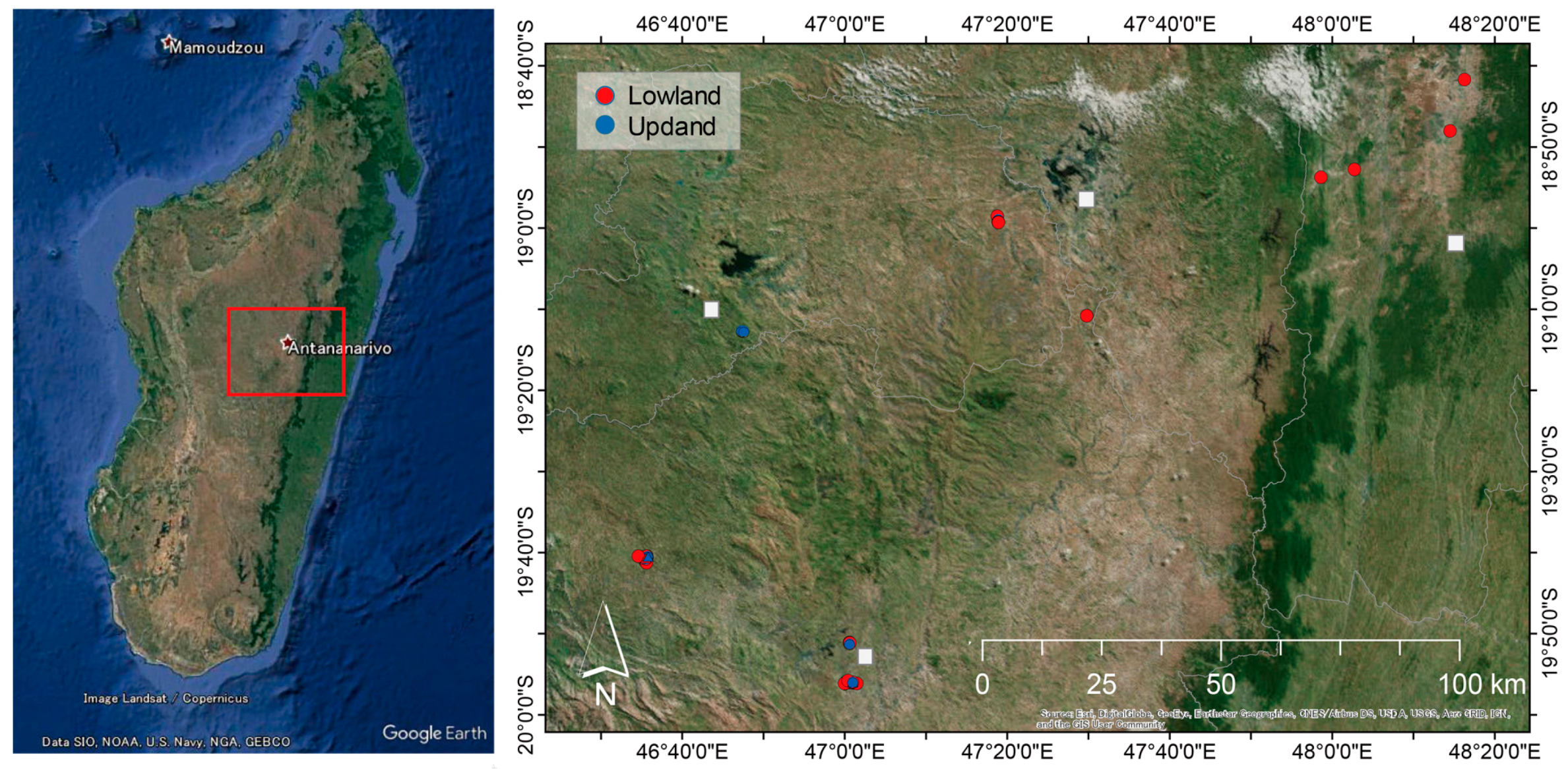
2.1. Study Site and Soil Sampling and Chemical Analyses

The field survey was conducted in the central highland of Madagascar (Figure 1). This region belongs to a subtropical climate with an altitude of 1000–1500 m above sea level. The mean temperature is 14–17 °C in winter and 20–22 °C in summer. The average annual rainfall is 1100 mm (>80% occurs in November–March) [33]. The area is dominated by inherently nutrient-poor soil types that are mainly classified into Ferralsols and Acrisols [39] or into Oxisols of semiarid to humid climates [40].
Soil sampling was conducted in 55 rice fields from August to November in 2016, consisting of eight upland and 47 lowland fields under various cropping systems (Figure 1). The sampling positions were recorded with a handy GPS (Colorado300, Garmin, Ltd., Kansas, TX, USA). Surface soil samples were collected from a 0–10 cm depth as composites of three to four cores in each field. Within three fields, sub-surface samples (10–20 cm depth in a field; 10–20, 20–30, and 30–40 cm depth in two fields) were also collected. Thus, 62 soil samples were obtained.

2.2. Soil Chemical Analyses

In the laboratory, soil samples were sieved to <2 mm and air dried for seven days. Earlier studies compared the effect of samples sieved to 2 mm and ground to 200 μm and did not obtain highly significant differences with respect to accuracy [41]. Thus, we worked with 2 mm crushed and sieved soil samples (0.6 g) in this study.
The TC and TN contents of soils were determined using an automatic NC analyzer, the SUMIGRAPH NC-220F (Sumika Chemical Analysis Service, Ltd., Osaka, Japan).

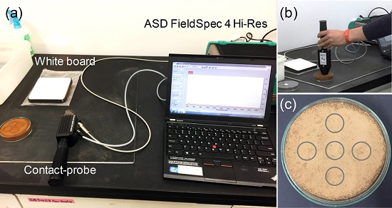
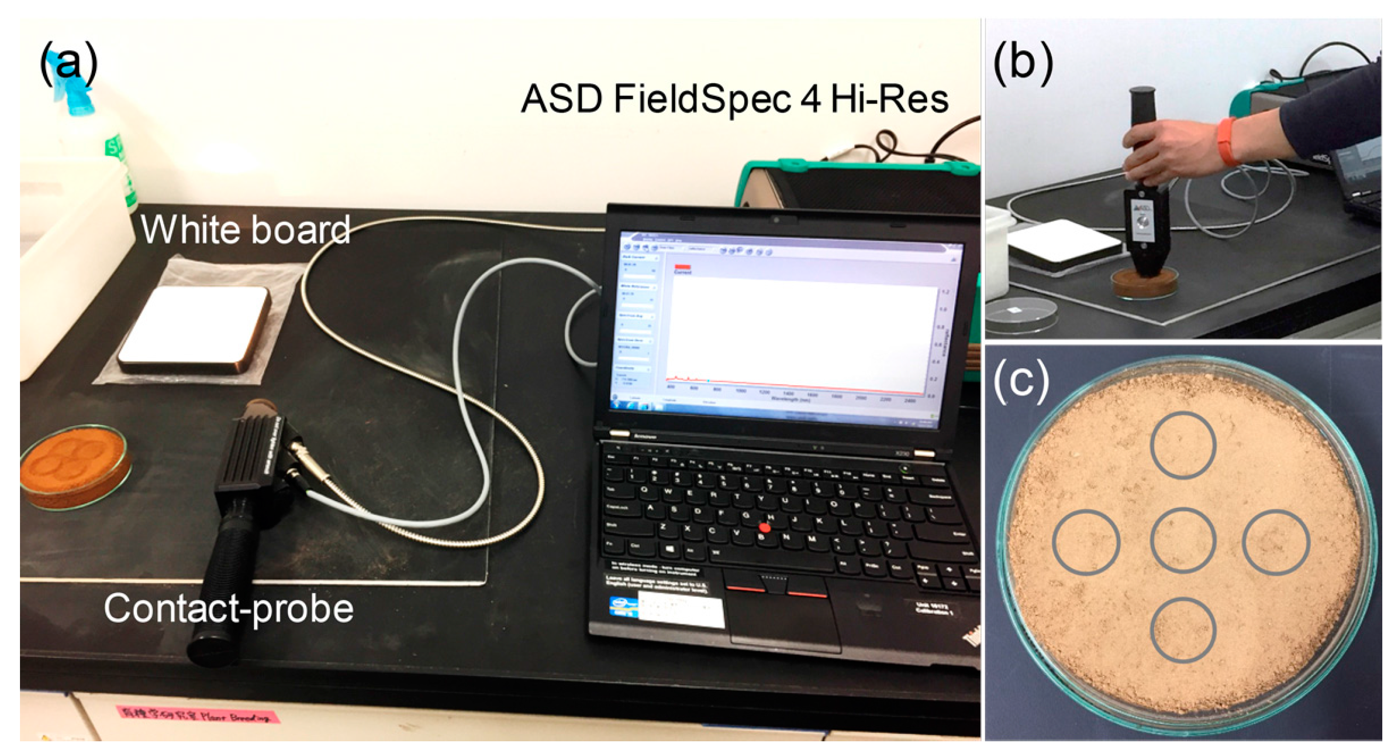
2.3. Vis-NIR Diffuse Reflectance Measurement

Laboratory soil reflectance measurements were conducted in a dark room at the Graduate School of Agriculture, Kyoto University, Japan, on 12–13 December 2016, using a portable spectro-radiometer (ASD FieldSpec 4 Hi-Res, ASD Inc., Longmont, CO, USA) and an ASD contact-probe (Figure 2). The ASD FieldSpec measures spectral reflectance in the 350–2500 nm wavelength region with spectral sampling of 1.4 nm in the 350–1000 nm range and 2 nm in the 1000–2500 nm range. The spectral resolution (full-width-half-maximum; FWHM) was 3 nm in the 350–1000 nm range and 6 nm in the 1000–2500 nm range, which were calculated to 1 nm resolution wavelengths for output data using the cubic spline interpolation function in ASD software (RS3 for Windows; ASD). The contact probe light source (halogen lamp) was aligned at 12° to the probe body, ensuring illumination at a fixed angle without the influence of ambient light. The fiber optic cable of the ASD FieldSpec was attached to the contact probe at a fixed measurement angle of 35°. The sensed spot area had a diameter of ~1.1 cm with a field of view of 1.33 cm2. A Spectralon (Labsphere, Inc., Sutton, NH, USA) reference panel (white reference) was used to optimize the ASD instrument prior to taking Vis-NIR reflectance measurements for each sample.
Bulk soil samples were spread in optical-glass Petri dishes 85 mm in diameter and pressed to form a layer ~19 mm tick. The soil surfaces were scanned 25 times with five replications for the soil samples (see Figure 2c), and the spectral readings were averaged.

2.4. Preprocessing of Spectral Data

Spectral data in both edge wavelength regions (350–399 nm and 2401–2500 nm) were eliminated because of low signal-to-noise ratios in the instrument. Thus, a total of 2001 spectral bands between 400 nm and 2400 nm were used for analyses.
First derivative reflectance (FDR) spectra were used to reduce baseline variation and enhance spectral features [42]. The FDR was calculated using the Savitzky-Golay smoothing filter [43]. A third-order, 15-band moving polynomial was fitted according to the original reflectance signatures. The parameters of this polynomial were subsequently used to calculate the derivative at the center waveband of the moving spline window. In addition, a standard normal variate transform (SNV) was employed to reduce the particle size effect [41].
To detect outliers, a principal component analysis was performed on spectral data for calculating the Mahalanobis distance H, and samples with H > 3 were eliminated as outliers. As a result, three samples were considered outliers, leaving 59 samples for further analyses.

2.5. Standard Full-Spectrum Partial Least Sqares (FS-PLS) Regression

PLS regression analyses were performed to estimate soil parameters using reflectance and FDR datasets (n = 59). The standard FS-PLS regression equation is as follows:
y = β 1 x 1 + β 2 x 2 + + β i x i + ε
where the response variable y is a vector of the soil parameters (TN and TC); the predictor variables x1 to xi are the surface reflectance or FDR values for spectral bands 1 to i (400, 401, …, 2400 nm), respectively; β1 to βi are the estimated weighted regression coefficients; and ε is the error vector. The latent variables were introduced to simplify the relationship between the response variables and predictor variables. To determine the optimal number of latent variables (NLV), leave-one-out (LOO) cross-validation was performed to avoid over-fitting of the model, which was based on the minimum value of the root mean squared error of cross-validation (RMSECV) (see in Supplementary Materials: Figure S1). The RMSECV was calculated as follows:
RMSECV = i = 1 n ( y i y p ) 2 n
where yi and yp represent the measured and predicted soil parameters for sample i, respectively, and n is the number of samples in the data sets (n = 59).

2.6. Iterative Stepwise Elimination Partial Least Squares (ISE-PLS) Regression

ISE-PLS is a PLS model that incorporates a waveband elimination algorithm. The ISE method eliminates noisy variables and selects useful predictors. When PLS models include large numbers of redundant variables or outliers, the models’ predictive abilities may perform poorly, while the ISE method can overcome such problems. Performance depends on the importance of predictors (zi), described as follows:
z i = | β i | s i i = 1 I | β i | s i
where si is the standard deviation and βi is the regression coefficient; both si and βi correspond to the predictor variable of the waveband i.
Initially, all available wavebands (2001 bands, 400–2400 nm) are used to develop the PLS regression model. Then, to create a scope in which useless predictor variables are removed and the predictive ability is improved, each predictor zi is evaluated, and the minimum values are eliminated as less informative wavebands. Subsequently, the PLS model is re-calibrated with the remaining predictors [44]. The model-building procedure is repeated until the final model is calibrated with the maximum predictive ability.

2.7. Predictive Ability of the PLS Models

The predictive abilities of the FS-PLS and ISE-PLS models were assessed by calculating the coefficient of determination (R2), RMSECV, and the residual predictive deviation (RPD) using LOO cross-validation. High R2 and low RMSECV values indicate the best model for predicting the soil parameters. The RPD has been defined as the ratio of standard deviation (SD) of reference data for predicting RMSECV [45]. For the performance ability of calibration models, RPD was suggested to be at least 3 for agriculture applications, while RPD values between 2 and 3 indicate a model with a good prediction ability, 1.5 < RPD < 2 is an intermediate model needing some improvement, and an RPD < 1.5 indicates that the model has a poor prediction ability [13].
To determine the significant wavelengths used in FS-PLS calibrations, the variable importance in the projection (VIP) [46,47] was used and referred to the selected wavelength regions from ISE-PLS models. The VIP score gives a summary of the importance of an x-variable (waveband) for an observed y-variable and is calculated using the following equation:
V I P k ( a ) = m a W a k 2 ( S S Y a S S Y t )
where VIPk(a) is the importance of the kth predictor variable based on a model with a factors, Wak is the corresponding loading weight of the kth variable in the ath PLS regression factor, SSYa is the explained sum of squares of y obtained from a PLS regression model with a factors, SSYt is the total sum of squares of y, and m is the total number of predictor variables. A high VIP score indicates an important x-variable (waveband) [46,48].
All the data handling and linear regression analyses were performed using MATLAB software ver. 9.0 (MathWorks, Sherborn, MA, USA).

3. Results and Discussion

3.1. Soil Properties (TC and TN) and Their Correlations with Each Waveband

Table 1 shows the descriptive analysis for soil TC and TN in the 59 samples. The mean (and SD) values of TC and TN were 2.18% (±1.16%) and 0.17% (±0.08%), respectively. The soil samples yielded a wide range of TC (coefficients of variation [CV] = 53.35) and TN values (CV = 48.08). The SD and range of sample affect the accuracy of soil property predictions using Vis-NIR spectroscopy [11]. In the present study, the ranges in soil TC and TN were considered sufficiently large to develop the calibration models using PLS regression analyses.
A significant correlation coefficient (r = 0.977, p < 0.001) was found between TC and TN in the soil samples. The results revealed that the soil TC and TN showed a similar shape of correlation using Vis-NIR reflectance and FDR spectra (see in Supplementary Materials: Figure S2). In the reflectance data, reflectance values at 1413 and 2207 nm were highly correlated with the soil TC and TN contents. A peak of negative correlation at 598 nm was also obtained in the Vis wavelength region. In a previous study [49], soil reflectance in the NIR wavelength region was characterized by well-defined absorption features associated with overtones of O-H and H-O-H stretch vibrations in free water (1455 and 1915 nm) and overtones and combinations of O-H stretch and metal-OH bends in a clay lattice (1415 and 2207 nm).

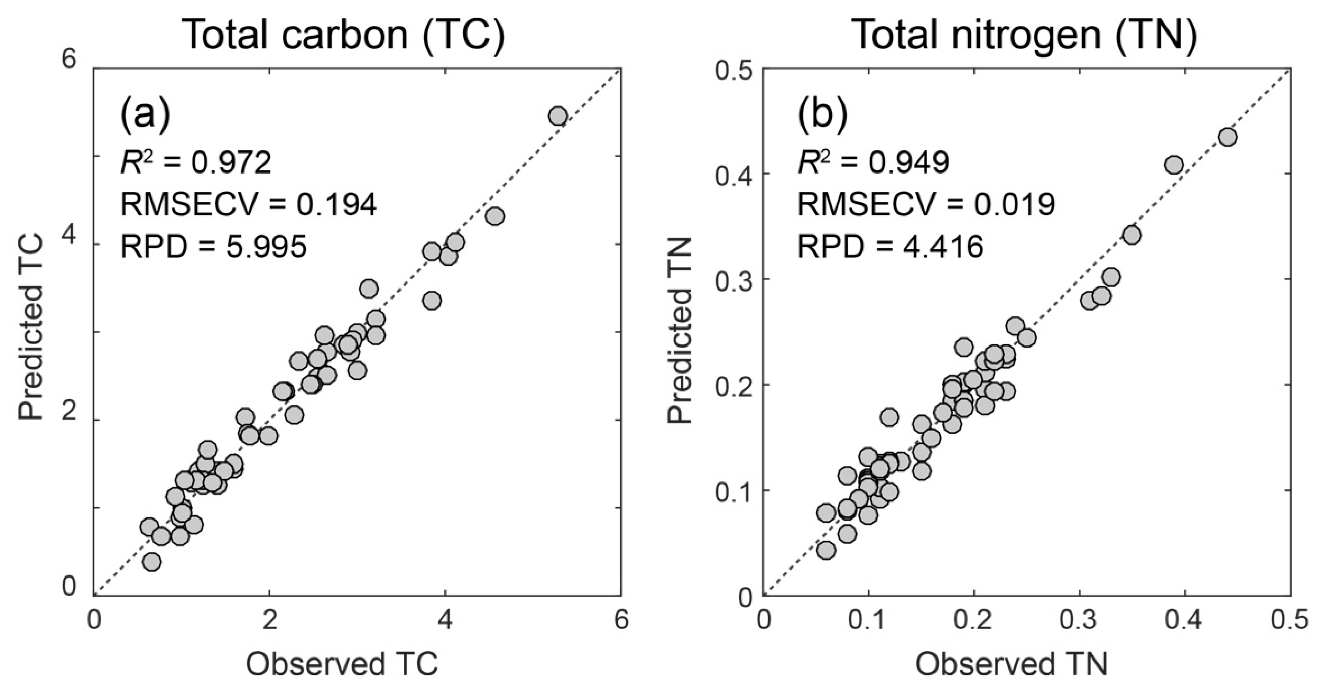
3.2. Comparison between FS-PLS and ISE-PLS Models

Figure 3 shows changes in the RMSECV and R2 values with iterative stepwise elimination procedures of redundant wavebands in the prediction of TC and TN using FDR. The RMSECV decreased as wavebands were removed but increased rapidly after more than 1749 and 1930 wavebands had been removed for TC and TN, respectively. Similarly, the R2 value tended to increase slowly until the maximum value was obtained when 1749 and 1930 wavebands had been removed. The remaining 252 (=2001 − 1749) and 71 (=2001 − 1930) wavebands were considered useful wavelengths for estimating TC and TN, respectively. The selected number of wavebands (NW) and the selected NW as a percentage of the full spectrum (NW% = NW/whole waveband [N = 2001]) are presented in Table 2, with the values of NLV, R2, RMSEC/CV, and RPD from the FS-PLS and ISE-PLS models using the FDR dataset. The optimum NLV ranged between 7 and 15, determined as the lowest RMSECV values calculated from LOO cross-validation to avoid over-fitting of the model.
Considering the difference in model accuracies between the FS-PLS and ISE-PLS (Table 2), better predictive accuracies were obtained in ISE-PLS than FS-PLS for both soil TC (R2 = 0.972, RMSECV = 0.194) and TN (R2 = 0.949, RMSECV = 0.019), with RPDs of 5.995 and 4.416, respectively. Figure 4 shows the relationships between the observed and cross-validated predicted values of soil TC and TN from ISE-PLS using FDR data. These results indicate that the soil TC and TN can be rapidly and accurately predicted from Vis-NIR diffuse reflectance spectroscopy using PLS regression. Selecting a subset of wavebands related to soil chemical properties and removing unrelated wavebands further improved the PLS regression results. Moreover, based on RPD > 3, the quality and future applicability of our results could be considered to have an excellent predictive ability. The remaining NW (NW%) of TC and TN was 252 (12.59%) and 71 (3.55%), respectively, suggesting that over 87% of the waveband information from the soil reflectance spectrum was redundant and did not contribute to or disturb the prediction of soil TC and TN.
These results agree with previous results indicating that the most useful information in the Vis-NIR region (400–2400 nm) was less than 20% for predicting forage [18,19] and water parameters [20]. These findings also support previous results showing that the performance of PLS models can be improved through waveband selection. Yang et al. [14] suggested that reducing large spectral datasets is valuable for more efficient storage, computation, and transmission, as well as for the ease of spectral analysis [50]. In addition, when fewer wavebands are used, simpler and cheaper spectro-radiometer processes can be developed.

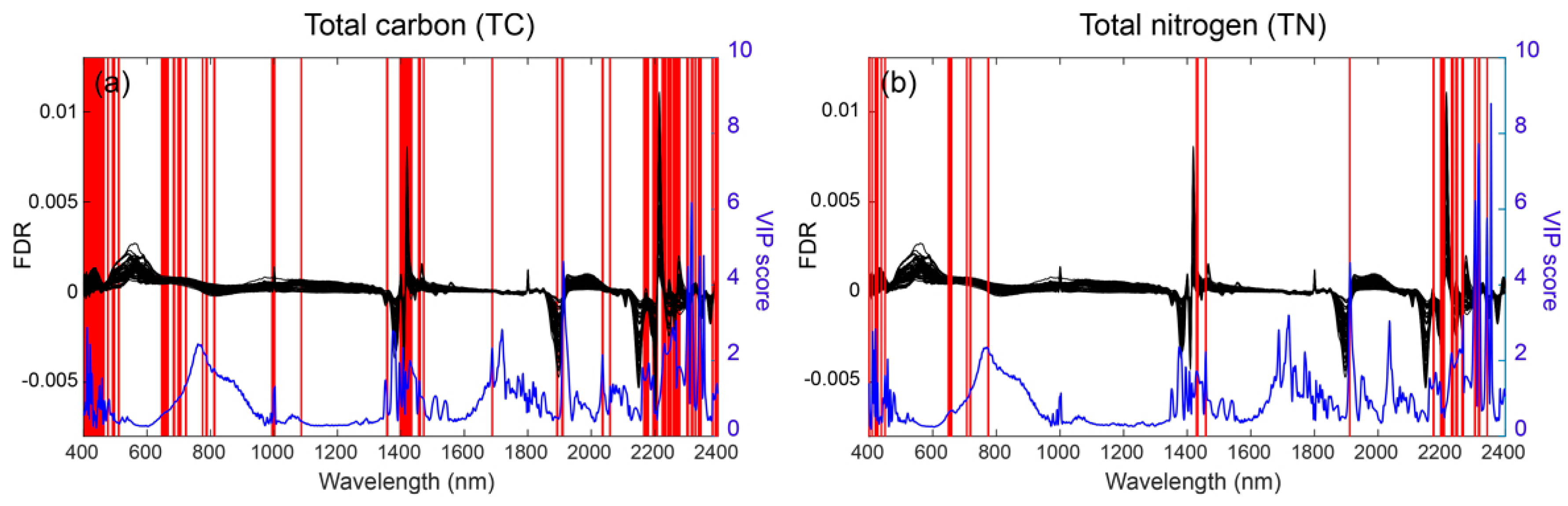
3.3. Selected Wavebands from ISE-PLS Models

The selected wavebands from ISE-PLS using FDR spectra to estimate soil TC and TN are shown in Figure 5, with VIP score values from FS-PLS. Based on the VIP score (>1), the wavelengths centered near 418, 470, 760, 1408, 1912, 2255, 2314, and 2339 nm were identified as common important wavelengths for estimating soil TC and TN. Most of the VIP peak regions were selected in the final ISE-PLS models. Although they did not perfectly fit with previously known absorption wavelength regions, some of the wavelengths were revealed within 30 nm of known absorption features. For soil TC prediction, the final model included Vis wavelength regions (400–480 and 640–700 nm), which are associated with soil color and had a huge influence on model calibration. Soil becomes darker as soil organic matter (SOM) increases; thus, several researchers have tried to use soil color information to estimate SOM [9,51]. However, soil darkness is only a useful discriminator within limited geological variation. In general, soil reflectance decreases with increasing organic matter content [49] and water content [52]. Absorptions of approximately 400, 450, 510, 550, 700, 870, and 1000 nm are characterized by the presence of ferrous and ferric iron oxides and are due to the electronic transitions of the iron cations [53]. A spectral band of 2100–2500 nm contributes to the model calibration of C and N in soils [54].
Martin et al. [55] reported that the NIR spectroscopy-based prediction of TN may be indirect due to a close correlation with TC, and that the calibration accuracy is higher for TC than for TN. Chang and Laird [56] confirmed that the NIR spectroscopy determination of TN does not always rely on a strong correlation with TC and can determine TN directly. Brunet et al. [41] hypothesized that, depending on the studied dataset, TN can be predicted based on its correlation with TC when the correlation is high; otherwise, it can be predicted directly. In our result, soil TC data showed a high correlation with soil TN data (r = 0.977), and calibrations obtained a better predictive accuracy for TC (R2 = 0.972, RMSECV = 0.194) than for TN (R2 = 0.949, RMSECV = 0.019). Within the selected wavebands of soil TN (Figure 5), 90.1% (=64/71 bands × 100%) overlapped with the selected wavebands of soil TC, whereas different wavebands in TC calibration were revealed mainly in the NIR region (707, 717–719, 774 nm). These results indicated that TN prediction using our dataset was affected by strong correlations with TC data but might be directly estimated.
Lastly, we note that this study was carried out on heterogenous sample data sets, which were collected at upland and lowland soils under various rice-based cropping systems, including wide ranges of soil types in Madagascar. However, several researchers consider the reliability of the prediction questionable when studying heterogeneous sample sets [41]. Particle size and arrangement might also affect the calibration due to the light transmission path [57]. Moreover, to map the carbon stock at a larger spatial scale in Madagascar, evaluating an appropriate spatial scale with a larger data set is required [58]. In future study, thus, more information concerning the effect of a heterogeneous data set on the accuracy of NIRS predictions at different scales is needed in order to apply the methodology to soil characterization of the whole island of Madagascar.

4. Conclusions

We investigated the performance of waveband selection in the spectral estimation of soil TC and TN using Vis-NIR reflectance data. The results indicated that soil TC and TN in Madagascar can be more accurately estimated by ISE-PLS than by standard FS-PLS using laboratory Vis-NIR spectroscopy. ISE-based wavelength selection in PLS calibration suggested that the important wavebands for estimating soil TC and TN were, respectively, 12.59% and 3.55% of all 2001 wavebands in the 400–2400 nm range. Based on selected FDR wavelengths in the ISE-PLS model, soil TC and TN were determined to provide excellent predictions (RPD > 3), with 0.194% and 0.019% error, respectively. The use of PLS with ISE waveband selection in Vis-NIR reflectance spectra is promising for the spectral assessment of soil TC and TN in Madagascar. Furthermore, the waveband selection procedure refined the predictive ability expected by optimizing the wavelength subset using ISE-PLS. Such timely and accurate soil TC and TN predictions might efficiently provide useful insights into fertilizer management.

Supplementary Materials

The following are available online at www.mdpi.com/2072-4292/9/10/1081/s1, Figure S1: Changes in RMSE (grey circle/line) and RMSECV (black circle/line) based on the number of latent variables (NLV) in models to estimate soil total carbon (TC) (a,c) and total nitrogen (TN) (b,d) using FS-PLS and ISE-PLS regressions. The optimal NLV (red vertical line) was determined the minimum value of RMSECV, Figure S2: Correlation coefficients (r) between soil chemical parameters (total carbon (C) and total nitrogen (TN)) at each wavelength: (a) reflectance and (b) first derivative reflectance (FDR).

Acknowledgments

This research was supported by the Science and Technology Research Partnership for Sustainable Development (SATREPS), Japan Science and Technology Agency (JST)/Japan International Cooperation Agency (JICA). We would like to give our special thanks to Naoki Moritsuka, Graduate School of Agriculture, Kyoto University in Japan, for his support in soil spectral measurement and for valuable comments on this manuscript.

Author Contributions

Kensuke Kawamura, Yasuhiro Tsujimoto, and Tovohery Rakotoson designed this study and the field work; Yasuhiro Tsujimoto, Michel Rabenarivo, Hidetoshi Asai, and Andry Andriamananjara performed the fieldwork and carried out the soil chemical analyses; Kensuke Kawamura performed laboratory spectral measurements and the data processing, and wrote the manuscript; and all the authors revised the paper.

Conflicts of Interest

The authors declare no conflict of interest.

References

  1. Weil, R.; Magdoff, F. Significance of soil organic matter to soil quality and health. In Soil Organic Matter in Sustainable Agriculture; Mangdoff, E., Weil, R.R., Eds.; CRC Press: Boca Raton, FL, USA, 2004; p. 412. [Google Scholar]
  2. Lal, R. Soil carbon sequestration to mitigate climate change. Geoderma 2004, 123, 1–22. [Google Scholar] [CrossRef]
  3. Mouazen, A.M.; Maleki, M.R.; De Baerdemaeker, J.; Ramon, H. On-line measurement of some selected soil properties using a vis–nir sensor. Soil Tillage Res. 2007, 93, 13–27. [Google Scholar] [CrossRef]
  4. Conant, R.T.; Ogle, S.M.; Paul, E.A.; Paustian, K. Measuring and monitoring soil organic carbon stocks in agricultural lands for climate mitigation. Front. Ecol. Environ. 2011, 9, 169–173. [Google Scholar] [CrossRef]
  5. Sinfield, J.V.; Fagerman, D.; Colic, O. Evaluation of sensing technologies for on-the-go detection of macro-nutrients in cultivated soils. Comput. Electron. Agric. 2010, 70, 1–18. [Google Scholar] [CrossRef]
  6. Conforti, M.; Castrignanò, A.; Robustelli, G.; Scarciglia, F.; Stelluti, M.; Buttafuoco, G. Laboratory-based vis–NIR spectroscopy and partial least square regression with spatially correlated errors for predicting spatial variation of soil organic matter content. Catena 2015, 124, 60–67. [Google Scholar] [CrossRef]
  7. Islam, K.; Singh, B.; McBratney, A. Simultaneous estimation of several soil properties by ultra-violet, visible, and near-infrared reflectance spectroscopy. Soil Res. 2003, 41, 1101–1114. [Google Scholar] [CrossRef]
  8. Miller, C.E. Chemical principles of near-infrared technology. In Near Infrared Technology in the Agricultural and Food Industries, 2nd ed.; Williams, P.C., Horris, K.H., Eds.; American Association of Cereal Chemists: St. Paul, MN, USA, 2001; pp. 19–37. [Google Scholar]
  9. Viscarra Rossel, R.A.; Walvoort, D.J.J.; McBratney, A.B.; Janik, L.J.; Skjemstad, J.O. Visible, near infrared, mid infrared or combined diffuse reflectance spectroscopy for simultaneous assessment of various soil properties. Geoderma 2006, 131, 59–75. [Google Scholar] [CrossRef]
  10. Mouazen, A.M.; Kuang, B.; De Baerdemaeker, J.; Ramon, H. Comparison among principal component, partial least squares and back propagation neural network analyses for accuracy of measurement of selected soil properties with visible and near infrared spectroscopy. Geoderma 2010, 158, 23–31. [Google Scholar] [CrossRef]
  11. Kuang, B.; Mouazen, A.M. Calibration of visible and near infrared spectroscopy for soil analysis at the field scale on three european farms. Eur. J. Soil Sci. 2011, 62, 629–636. [Google Scholar] [CrossRef]
  12. Fystro, G. The prediction of C and N content and their potential mineralisation in heterogeneous soil samples using vis–nir spectroscopy and comparative methods. Plant Soil 2002, 246, 139–149. [Google Scholar] [CrossRef]
  13. 13 D’Acqui, L.P.; Pucci, A.; Janik, L.J. Soil properties prediction of western mediterranean islands with similar climatic environments by means of mid-infrared diffuse reflectance spectroscopy. Eur. J. Soil Sci. 2010, 61, 865–876. [Google Scholar] [CrossRef]
  14. Yang, H.; Kuang, B.; Mouazen, A.M. Quantitative analysis of soil nitrogen and carbon at a farm scale using visible and near infrared spectroscopy coupled with wavelength reduction. Eur. J. Soil Sci. 2012, 63, 410–420. [Google Scholar] [CrossRef]
  15. Vohland, M.; Ludwig, M.; Thiele-Bruhn, S.; Ludwig, B. Determination of soil properties with visible to near- and mid-infrared spectroscopy: Effects of spectral variable selection. Geoderma 2014, 223, 88–96. [Google Scholar] [CrossRef]
  16. Inoue, Y.; Sakaiya, E.; Zhu, Y.; Takahashi, W. Diagnostic mapping of canopy nitrogen content in rice based on hyperspectral measurements. Remote Sens. Environ. 2012, 126, 210–221. [Google Scholar] [CrossRef]
  17. Bolster, K.L.; Martin, M.E.; Aber, J.D. Determination of carbon fraction and nitrogen concentration in tree foliage by near infrared reflectance: A comparison of statistical methods. Can. J. For. Res. 1996, 26, 590–600. [Google Scholar] [CrossRef]
  18. Kawamura, K.; Watanabe, N.; Sakanoue, S.; Lee, H.-J.; Inoue, Y.; Odagawa, S. Testing genetic algorithm as a tool to select relevant wavebands from field hyperspectral data for estimating pasture mass and quality in a mixed sown pasture using partial least squares regression. Grassl. Sci. 2010, 56, 205–216. [Google Scholar] [CrossRef]
  19. Kawamura, K.; Watanabe, N.; Sakanoue, S.; Lee, H.-J.; Lim, J.; Yoshitoshi, R. Genetic algorithm-based partial least squares regression for estimating legume content in a grass-legume mixture using field hyperspectral measurements. Grassl. Sci. 2013, 59, 166–172. [Google Scholar] [CrossRef]
  20. Wang, Z.; Kawamura, K.; Sakuno, Y.; Fan, X.; Gong, Z.; Lim, J. Retrieval of chlorophyll-a and total suspended solids using iterative stepwise elimination partial least squares (ISE-PLS) regression based on field hyperspectral measurements in irrigation ponds in higashihiroshima, Japan. Remote Sens. 2017, 9, 264. [Google Scholar] [CrossRef]
  21. Fan, W.; Shan, Y.; Li, G.; Lv, H.; Li, H.; Liang, Y. Application of competitive adaptive reweighted sampling method to determine effective wavelengths for prediction of total acid of vinegar. Food Anal. Meth. 2012, 5, 585–590. [Google Scholar] [CrossRef]
  22. Cramer, J.A.; Kramer, K.E.; Johnson, K.J.; Morris, R.E.; Rose-Pehrsson, S.L. Automated wavelength selection for spectroscopic fuel models by symmetrically contracting repeated unmoving window partial least squares. Chemom. Intell. Lab. Syst. 2008, 92, 13–21. [Google Scholar] [CrossRef]
  23. Kawamura, K.; Watanabe, N.; Sakanoue, S.; Inoue, Y. Estimating forage biomass and quality in a mixed sown pasture based on pls regression with waveband selection. Grassl. Sci. 2008, 54, 131–146. [Google Scholar] [CrossRef]
  24. Boggia, R.; Forina, M.; Fossa, P.; Mosti, L. Chemometric study and validation strategies in the structure-activity relationships of new cardiotonic agents. Quant. Struct.-Act. Relatsh. 1997, 16, 201–213. [Google Scholar] [CrossRef]
  25. Centner, V.; Massart, D.L.; de Noord, O.E.; de Jong, S.; Vandeginste, B.M.; Sterna, C. Elimination of uninformative variables for multivariate calibration. Anal. Chem. 1996, 68, 3851–3858. [Google Scholar] [CrossRef] [PubMed]
  26. Li, H.; Liang, Y.; Xu, Q.; Cao, D. Key wavelengths screening using competitive adaptive reweighted sampling method for multivariate calibration. Anal. Chim. Acta 2009, 648, 77–84. [Google Scholar] [CrossRef] [PubMed]
  27. Nørgaard, L.; Saudland, A.; Wagner, J.; Nielsen, J.P.; Munck, L.; Engelsen, S.B. Interval partial least-squares regression (iPLS): A comparative chemometric study with an example from near-infrared spectroscopy. Appl. Spectrosc. 2000, 54, 413–419. [Google Scholar] [CrossRef]
  28. Jiang, J.H.; Berry, R.J.; Siesler, H.W.; Ozaki, Y. Wavelength interval selection in multicomponent spectral analysis by moving window partial least-squares regression with applications to mid-infrared and near-infrared spectroscopic data. Anal. Chem. 2002, 74, 3555–3565. [Google Scholar] [CrossRef] [PubMed]
  29. Leardi, R. Application of a genetic algorithm to feature selection under full validation conditions and to outlier detection. J. Chemom. 1994, 8, 65–79. [Google Scholar] [CrossRef]
  30. Yoshida, H.; Leardi, R.; Funatsu, K.; Varmuza, K. Feature selection by genetic algorithms for mass spectral classifiers. Anal. Chim. Acta 2001, 446, 483–492. [Google Scholar] [CrossRef]
  31. Xiaobo, Z.; Jiewen, Z.; Povey, M.J.W.; Holmes, M.; Hanpin, M. Variables selection methods in near-infrared spectroscopy. Anal. Chim. Acta 2010, 667, 14–32. [Google Scholar] [CrossRef] [PubMed]
  32. GriSP (Global Rice Science Partnership). Rice Almanac, 4th ed.; International Rice Research Institute: Los Banos, Philippines, 2013; p. 298. [Google Scholar]
  33. Tsujimoto, Y.; Horie, T.; Randriamihary, H.; Shiraiwa, T.; Homma, K. Soil management: The key factors for higher productivity in the fields utilizing the system of rice intensification (SRI) in the central highland of madagascar. Agric. Syst. 2009, 100, 61–71. [Google Scholar] [CrossRef]
  34. Grinand, C.; Maire, G.L.; Vieilledent, G.; Razakamanarivo, H.; Razafimbelo, T.; Bernoux, M. Estimating temporal changes in soil carbon stocks at ecoregional scale in madagascar using remote-sensing. Int. J. Appl. Earth Obs. Geoinf. 2017, 54, 1–14. [Google Scholar] [CrossRef]
  35. Ramifehiarivo, N.; Brossard, M.; Grinand, C.; Andriamananjara, A.; Razafimbelo, T.; Rasolohery, A.; Razafimahatratra, H.; Seyler, F.; Ranaivoson, N.; Rabenarivo, M.; et al. Mapping soil organic carbon on a national scale: Towards an improved and updated map of madagascar. Geoderma Reg. 2017, 9, 29–38. [Google Scholar] [CrossRef]
  36. Razakamanarivo, R.H.; Grinand, C.; Razafindrakoto, M.A.; Bernoux, M.; Albrecht, A. Mapping organic carbon stocks in eucalyptus plantations of the Central Highlands of Madagascar: A multiple regression approach. Geoderma 2011, 162, 335–346. [Google Scholar] [CrossRef]
  37. Andriamananjara, A.; Hewson, J.; Razakamanarivo, H.; Andrisoa, R.H.; Ranaivoson, N.; Ramboatiana, N.; Razafindrakoto, M.; Ramifehiarivo, N.; Razafimanantsoa, M.-P.; Rabeharisoa, L.; et al. Land cover impacts on aboveground and soil carbon stocks in malagasy rainforest. Agric. Ecosyst. Environ. 2016, 233, 1–15. [Google Scholar] [CrossRef]
  38. Asner, G.P.; Mascaro, J.; Muller-Landau, H.C.; Vieilledent, G.; Vaudry, R.; Rasamoelina, M.; Hall, J.S.; van Breugel, M. A universal airborne lidar approach for tropical forest carbon mapping. Oecologia 2012, 168, 1147–1160. [Google Scholar] [CrossRef] [PubMed]
  39. IUSS Working Group WRB. World Reference Base for Soil Resources 2014, Update 2015 International Soil Classification System for Naming Soils and Creating Legends for Soil Maps; World Soil Resources Reports No. 106; FAO: Rome, Italy, 2015. [Google Scholar]
  40. Soil Survey Staff. Keys to Soil Taxonomy, 12th ed.; USDA-Natural Resources Cnservation Service: Washington, DC, USA, 2014. [Google Scholar]
  41. Brunet, D.; Barthès, B.G.; Chotte, J.-L.; Feller, C. Determination of carbon and nitrogen contents in alfisols, oxisols and ultisols from africa and brazil using nirs analysis: Effects of sample grinding and set heterogeneity. Geoderma 2007, 139, 106–117. [Google Scholar] [CrossRef]
  42. Reeves, J.; McCarty, G.; Mimmo, T. The potential of diffuse reflectance spectroscopy for the determination of carbon inventories in soils. Environ. Pollut. 2002, 116, S277–S284. [Google Scholar] [CrossRef]
  43. Savitzky, A.; Golay, M.J.E. Smoothing and differentiation of data by simplified least squares procedures. Anal. Chem. 1964, 36, 1627–1639. [Google Scholar] [CrossRef]
  44. Forina, M.; Lanteri, S.; Oliveros, M.C.C.; Millan, C.P. Selection of useful predictors in multivariate calibration. Anal. Bioanal. Chem. 2004, 380, 397–418. [Google Scholar] [CrossRef] [PubMed]
  45. Williams, P.C. Implementation of near-infrared technology. In Near-Infrared Technology in the Agricultural and Food Industries, 2nd ed.; Williams, P.C., Norris, K.H., Eds.; American Association of Cereal Chemists Inc.: St. Paul, MN, USA, 2001; pp. 145–169. [Google Scholar]
  46. Wold, S.; Sjöström, M.; Eriksson, L. PLS-regression: A basic tool of chemometrics. Chemom. Intell. Lab. Syst. 2001, 58, 109–130. [Google Scholar] [CrossRef]
  47. Chong, I.-G.; Jun, C.-H. Performance of some variable selection methods when multicollinearity is present. Chemom. Intell. Lab. Syst. 2005, 78, 103–112. [Google Scholar] [CrossRef]
  48. Li, B.; Liew, O.W.; Asundi, A.K. Pre-visual detection of iron and phosphorus deficiency by transformed reflectance spectra. J. Photochem. Photobiol. B 2006, 85, 131–139. [Google Scholar] [CrossRef] [PubMed]
  49. Ben-Dor, E.; Inbar, Y.; Chen, Y. The reflectance spectra of organic matter in the visible near-infrared and short wave infrared region (400–2500 nm) during a controlled decomposition process. Remote Sens. Environ. 1997, 61, 1–15. [Google Scholar] [CrossRef]
  50. Viscarra Rossel, R.A.; Lark, R.M. Improved analysis and modelling of soil diffuse reflectance spectra using wavelets. Eur. J. Soil Sci. 2009, 60, 453–464. [Google Scholar] [CrossRef]
  51. Viscarra Rossel, R.A.; Fouad, Y.; Walter, C. Using a digital camera to measure soil organic carbon and iron contents. Biosyst. Eng. 2008, 100, 149–159. [Google Scholar] [CrossRef]
  52. Whiting, M.L.; Li, L.; Ustin, S.L. Predicting water content using gaussian model on soil spectra. Remote Sens. Environ. 2004, 89, 535–552. [Google Scholar] [CrossRef]
  53. Ben Dor, E.; Irons, J.R.; Epema, J.F. Soil reflectance. In Manual of Remote Sensing: Remote Sensing for the Earth Sciences; John Wiley & Sons: New York, NY, USA, 1999; Volume 3, pp. 111–188. [Google Scholar]
  54. Yang, H. Spectroscopic calibration for soil N and C measurement at a farm scale. Proc. Environ. Sci. 2011, 10, 672–677. [Google Scholar] [CrossRef]
  55. Martin, P.D.; Malley, D.F.; Manning, G.; Fuller, L. Determination of soil organic carbon and nitrogen at the field level using near-infrared spectroscopy. Can. J. Soil Sci. 2002, 82, 413–422. [Google Scholar] [CrossRef]
  56. Chang, C.-W.; Laird, D.A. Near-infrared reflectance spectroscopic analysis of soil C and N. Soil Sci. 2002, 167, 110–116. [Google Scholar] [CrossRef]
  57. Chang, C.W.; Laird, D.; Mausbach, M.J.; Hurburgh, C.R.J. Nearinfrared reflectance spectroscopy-principal components regression analyses of soil properties. Soil Sci. Soc. Am. J. 2001, 65, 480–490. [Google Scholar] [CrossRef]
  58. Saiano, F.; Oddo, G.; Scalenghe, R.; La Mantia, T.; Ajmone-Marsan, F. DRIFTS sensor: Soil carbon validation at large scale (Pantelleria, Italy). Sensors 2013, 13, 5603–5613. [Google Scholar] [CrossRef] [PubMed] [Green Version]
Figure 1. Locations of studied regions and soil sampling points.
Remotesensing 09 01081 g001
Figure 2. (a) The setup used to measure the soil reflectance in a dark room; (b) the use of a contact probe that touches the surface of the soil sample; and (c) the five measuring spots on a soil sample.
Remotesensing 09 01081 g002
Figure 3. Changes in RMSECV (black line) and R2 values (red line) in models to estimate total carbon (TC) (a) and total nitrogen (TN) (b) with the stepwise removal of redundant wavebands. The minimum value of the root mean squared error of cross-validation (RMSECV) (blue dotted line) was obtained when 1749 and 1930 wavebands were removed for TC and TN, respectively.
Remotesensing 09 01081 g003
Figure 4. Observed and predicted values of soil total carbon (TC) and soil total nitrogen (TN) contents using ISE-PLS models with first derivative reflectance (FDR) data (n = 59). The coefficient of determination (R2), root mean squared error of cross-validation (RMSECV), and residual predicted value (RPD) are cross-validated (leave-one-out cross-validation method) coefficient of determination, root mean squared error, and residual predictive values, respectively (see Table 2).
Remotesensing 09 01081 g004
Figure 5. Soil reflectance and its first derivative reflectance (FDR) spectra for the total carbon (TC; a) and total nitrogen (TN; b) datasets and selected waveband (red bar) in iterative stepwise elimination of partial least squares (ISE-PLS) with variable importance in the prediction (VIP) score (blue line) from full-spectrum PLS (FSPLS) models.
Remotesensing 09 01081 g005
Table 1. Descriptive statistics of soil sample data.
Soil ParametersnMinMaxMeanSDCV
TC (%)590.656.022.181.1653.35
TN (%)590.060.440.170.0848.08
n, number of samples; SD, standard deviation; CV, coefficient of variation (=Mean/SD × 100%).
Table 2. Optimum number of latent variables (NLV), coefficient of determination (R2), root mean squared errors of calibration (RMSEC) and cross-validation (RMSECV), and residual predictive values (RPD) from full-spectrum PLS (FS-PLS) and iterative stepwise elimination PLS (ISE-PLS) models with a selected number of wavebands (NW) and their percentages of the full spectrum (NW%).
Soil ParameterRegression MethodCalibrationCross-validationNWNW%
NLVR2RMSECR2RMSECVRPD
Total carbonFS-PLS140.9960.0760.8930.3793.06425212.59
(TC, %)ISE-PLS120.9950.0840.9720.1945.995
Total nitrogenFS-PLS90.9600.0160.8370.0332.480713.55
(TN, %)ISE-PLS70.9740.0130.9490.0194.416
FS-PLS, full-spectrum partial least squares; ISE-PLS, iterative stepwise elimination PLS; NLV, number of latent variables: RMSEC (or RMSECV), root mean squared error of calibration (or cross-validation); NW, number of wavebands; NW%, number of waveband percentages of all available bands (=NW/2001 bands × 100%).

