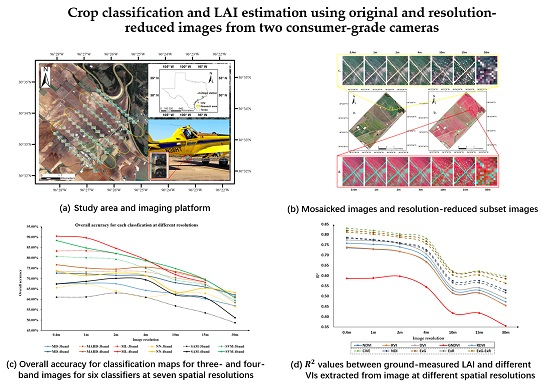
Crop Classification and LAI Estimation Using Original and Resolution-Reduced Images from Two Consumer-Grade Cameras

 ,
,
Abstract
:
1. Introduction
2. Materials and Methods
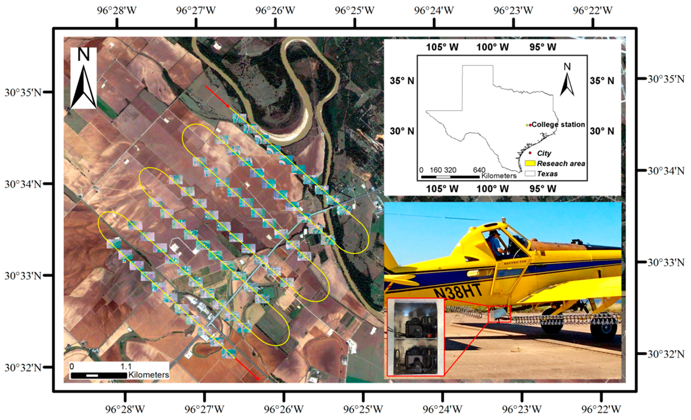
2.1. Study Area
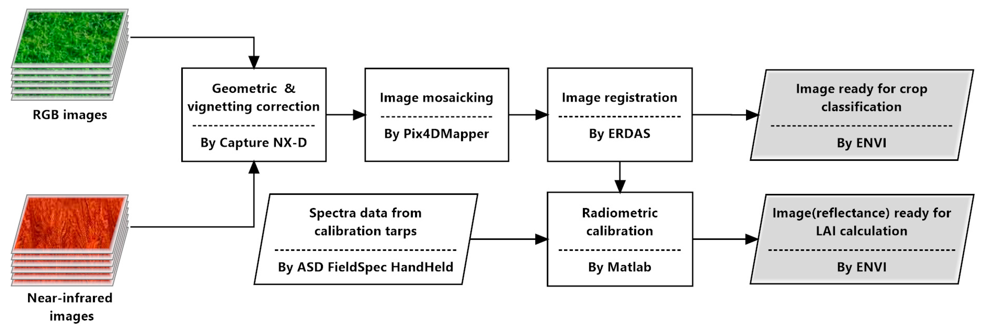
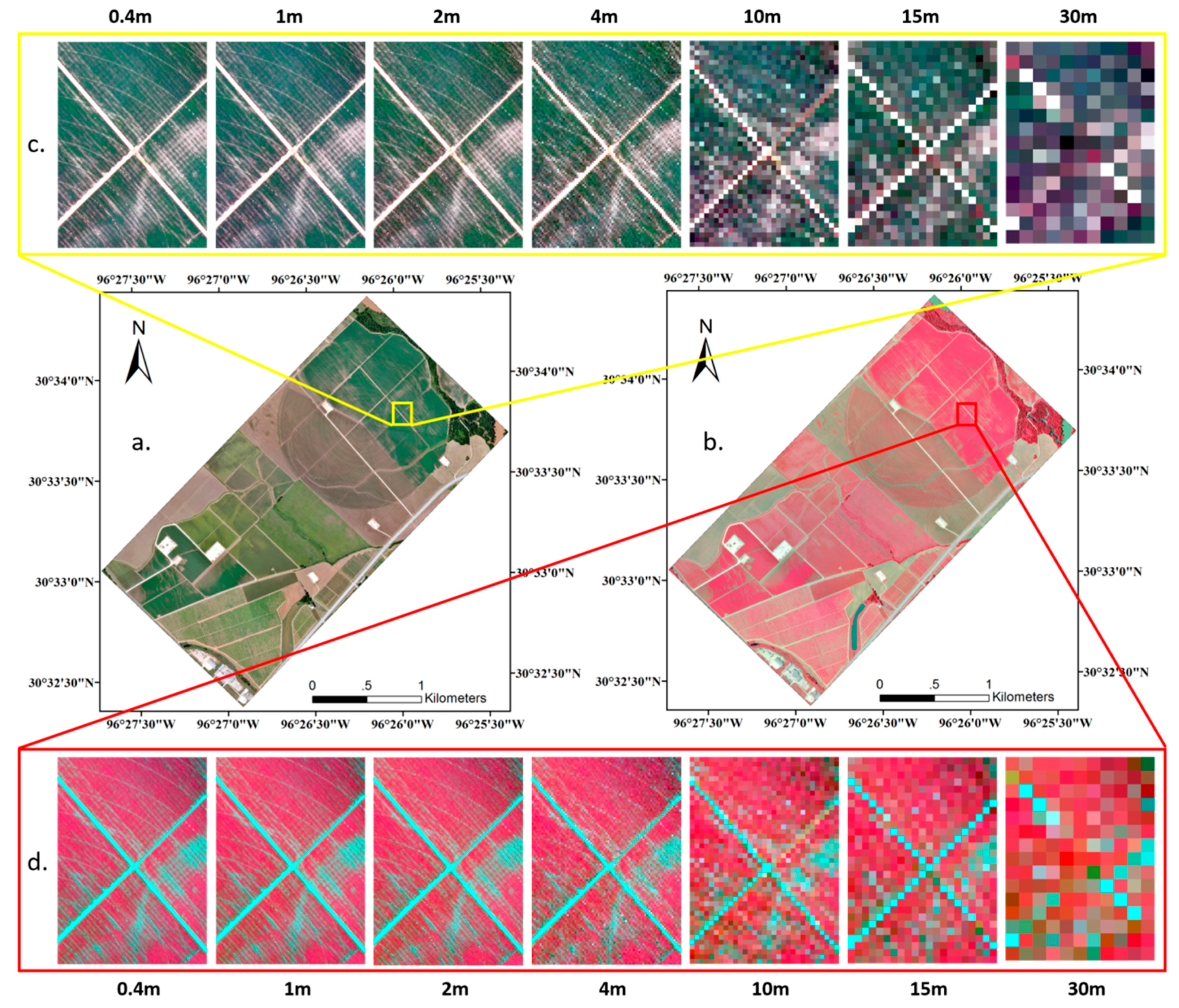
2.2. Image Pre-Processing
2.3. Crop Identification
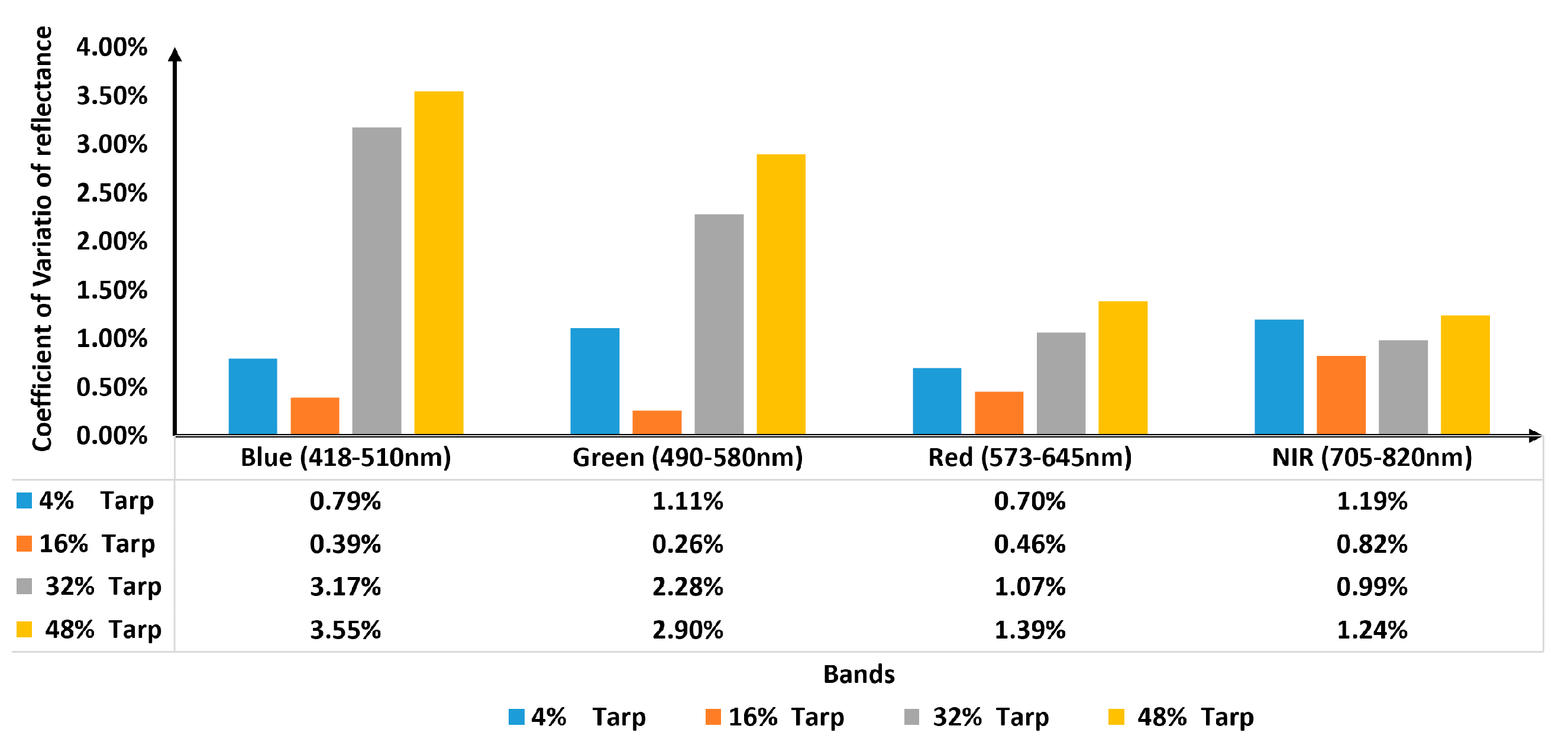
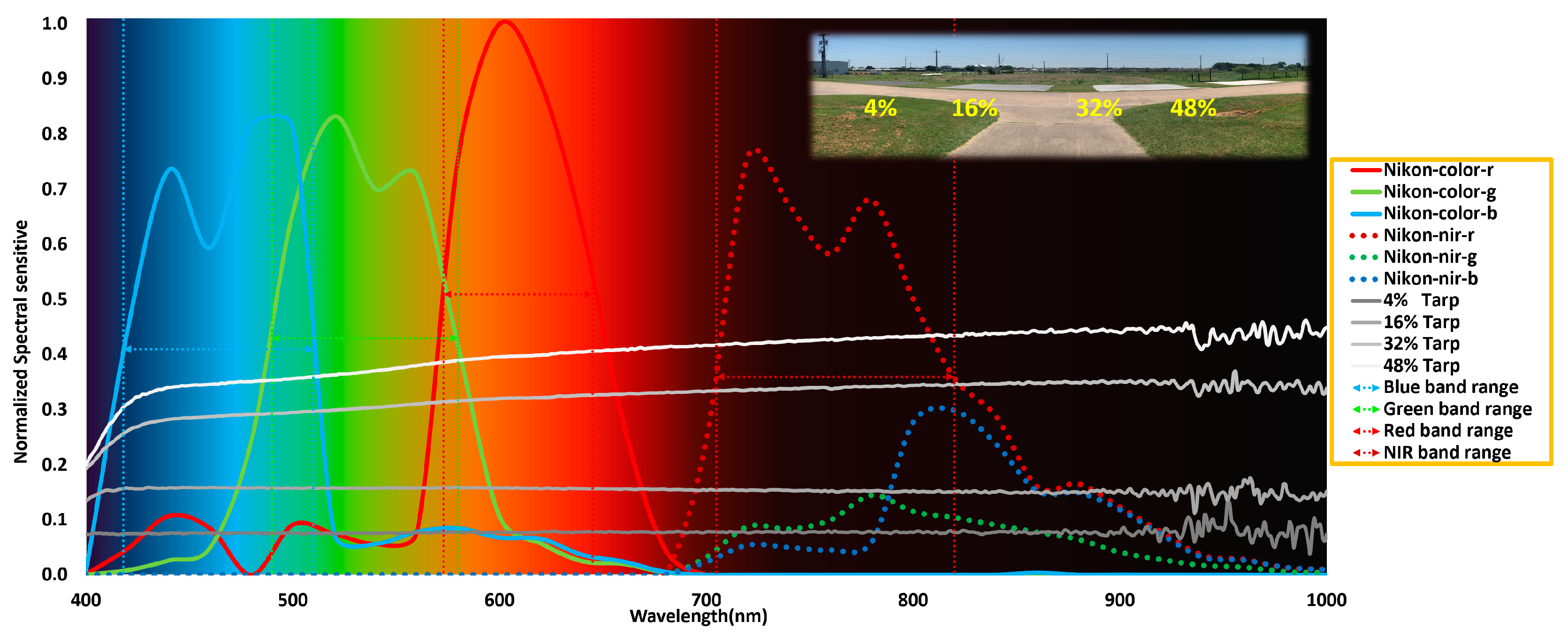
2.4. LAI Data Collection and Radiometric Calibration
3. Results and Discussion
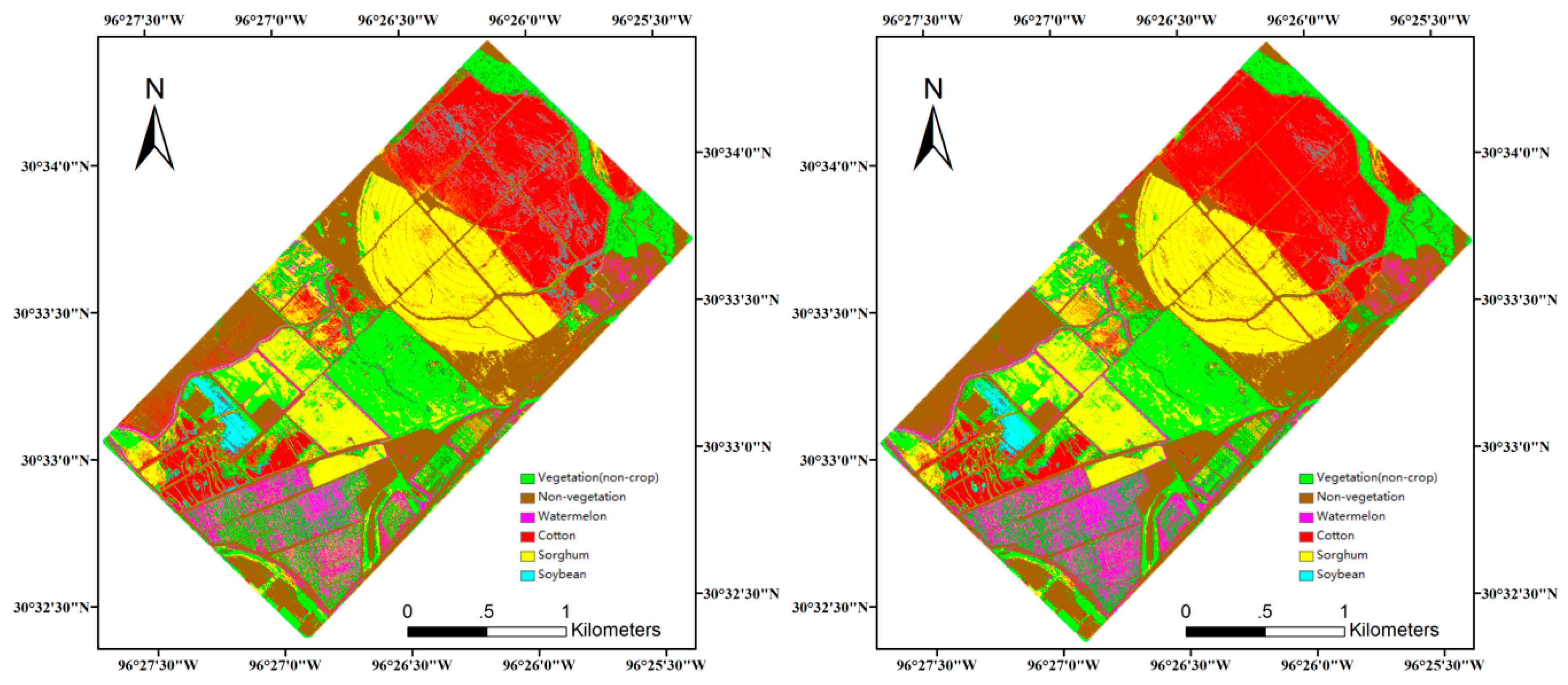
3.1. Crop Classification
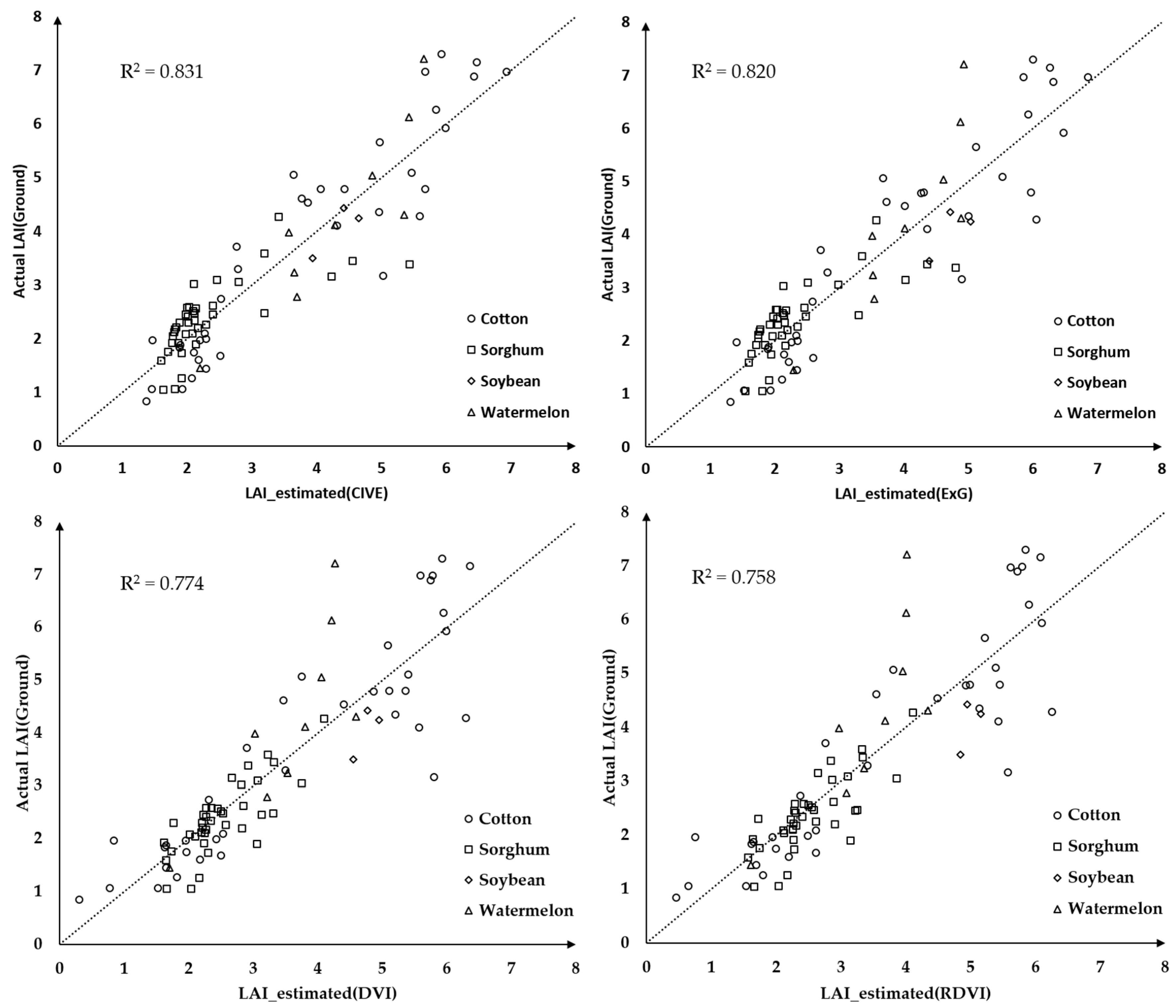
3.2. Crop LAI Assessment Application
4. Conclusions
Supplementary Materials
Supplementary File 1Acknowledgments
Author Contributions
Conflicts of Interest
Disclaimer
References
- Schimmelpfennig, D.; Ebel, R. Sequential adoption and cost savings from precision agriculture. J. Agric. Resour. Econ. 2016, 41, 97–115. [Google Scholar]
- Nijland, W.; de Jong, R.; de Jong, S.M.; Wulder, M.A.; Bater, C.W.; Coops, N.C. Monitoring plant condition and phenology using infrared sensitive consumer grade digital cameras. Agric. For. Meteorol. 2014, 184, 98–106. [Google Scholar] [CrossRef]
- Light, D.L. Film cameras or digital sensors? The challenge ahead for aerial imaging. Photogramm. Eng. Remote Sens. 1996, 62, 285–291. [Google Scholar]
- Quilter, M.C.; Anderson, V.J. Low altitude/large scale aerial photographs: A tool for range and resource managers. Rangel. Arch. 2000, 22, 13–17. [Google Scholar] [CrossRef]
- Yuan, H.; Yang, G.; Li, C.; Wang, Y.; Liu, J.; Yu, H.; Feng, H.; Xu, B.; Zhao, X.; Yang, X. Retrieving soybean leaf area index from unmanned aerial vehicle hyperspectral remote sensing: Analysis of RF, ANN, and SVM regression models. Remote Sens. 2017, 9, 309. [Google Scholar] [CrossRef]
- Yang, C.; Odvody, G.N.; Thomasson, J.A.; Isakeit, T.; Nichols, R.L. Change detection of cotton root rot infection over 10-year intervals using airborne multispectral imagery. Comput. Electron. Agric. 2016, 123, 154–162. [Google Scholar] [CrossRef]
- Yang, C.; Westbrook, J.K.; Suh, C.P.-C.; Martin, D.E.; Hoffmann, W.C.; Lan, Y.; Fritz, B.K.; Goolsby, J.A. An airborne multispectral imaging system based on two consumer-grade cameras for agricultural remote sensing. Remote Sens. 2014, 6, 5257–5278. [Google Scholar] [CrossRef]
- Hu, Z.; He, F.; Yin, J.; Lu, X.; Tang, S.; Wang, L.; Li, X. Estimation of fractional vegetation cover based on digital camera survey data and a remote sensing model. J. China Univ. Min. Echnol. 2007, 17, 116–120. [Google Scholar] [CrossRef]
- Zarco-Tejada, P.J.; Diaz-Varela, R.; Angileri, V.; Loudjani, P. Tree height quantification using very high resolution imagery acquired from an unmanned aerial vehicle (uav) and automatic 3d photo-reconstruction methods. Eur. J. Agron. 2014, 55, 89–99. [Google Scholar] [CrossRef]
- Prosdocimi, M.; Calligaro, S.; Sofia, G.; Dalla Fontana, G.; Tarolli, P. Bank erosion in agricultural drainage networks: New challenges from structure-from-motion photogrammetry for post-event analysis. Earth Surf. Process. Landf. 2015, 40, 1891–1906. [Google Scholar] [CrossRef]
- Prosdocimi, M.; Burguet, M.; Di Prima, S.; Sofia, G.; Terol, E.; Rodrigo Comino, J.; Cerdà, A.; Tarolli, P. Rainfall simulation and structure-from-motion photogrammetry for the analysis of soil water erosion in mediterranean vineyards. Sci. Total Environ. 2017, 574, 204–215. [Google Scholar] [CrossRef] [PubMed]
- Shi, Y.; Thomasson, J.A.; Murray, S.C.; Pugh, N.A.; Rooney, W.L.; Shafian, S.; Rajan, N.; Rouze, G.; Morgan, C.L.S.; Neely, H.L.; et al. Unmanned aerial vehicles for high-throughput phenotyping and agronomic research. PLoS ONE 2016, 11, e0159781. [Google Scholar] [CrossRef] [PubMed]
- Yang, C.; Hoffmann, W.C. Low-cost single-camera imaging system for aerial applicators. J. Appl. Remote Sens. 2015, 9, 096064. [Google Scholar] [CrossRef]
- Wellens, J.; Midekor, A.; Traore, F.; Tychon, B. An easy and low-cost method for preprocessing and matching small-scale amateur aerial photography for assessing agricultural land use in burkina faso. Int. J. Appl. Earth Obs. Geoinf. 2013, 23, 273–278. [Google Scholar] [CrossRef]
- Diaz-Varela, R.; Zarco-Tejada, P.J.; Angileri, V.; Loudjani, P. Automatic identification of agricultural terraces through object-oriented analysis of very high resolution dsms and multispectral imagery obtained from an unmanned aerial vehicle. J. Environ. Manag. 2014, 134, 117–126. [Google Scholar] [CrossRef] [PubMed]
- Jensen, T.; Apan, A.; Young, F.; Zeller, L. Detecting the attributes of a wheat crop using digital imagery acquired from a low-altitude platform. Comput. Electron. Agric. 2007, 59, 66–77. [Google Scholar] [CrossRef] [Green Version]
- Colomina, I.; Molina, P. Unmanned aerial systems for photogrammetry and remote sensing: A review. ISPRS J. Photogramm. Remote Sens. 2014, 92, 79–97. [Google Scholar] [CrossRef]
- Bayer, B.E. Color Imaging Array. US Patent, 3,971,065, 20 July 1976. [Google Scholar]
- Lelong, C.C.D. Assessment of unmanned aerial vehicles imagery for quantitative monitoring of wheat crop in small plots. Sensors 2008, 8, 3557–3585. [Google Scholar] [CrossRef] [PubMed]
- Miller, C.D.; Fox-Rabinovitz, J.R.; Allen, N.F.; Carr, J.L.; Kratochvil, R.J.; Forrestal, P.J.; Daughtry, C.S.T.; McCarty, G.W.; Hively, W.D.; Hunt, E.R. Nir-green-blue high-resolution digital images for assessment of winter cover crop biomass. GISci. Remote Sens. 2011, 48, 86–98. [Google Scholar]
- Akkaynak, D.; Treibitz, T.; Xiao, B.; Gürkan, U.A.; Allen, J.J.; Demirci, U.; Hanlon, R.T. Use of commercial off-the-shelf digital cameras for scientific data acquisition and scene-specific color calibration. JOSA A 2014, 31, 312–321. [Google Scholar] [CrossRef] [PubMed]
- Song, H.; Yang, C.; Zhang, J.; Hoffmann, W.C.; He, D.; Thomasson, J.A. Comparison of mosaicking techniques for airborne images from consumer-grade cameras. J. Appl. Remote Sens. 2016, 10, 016030. [Google Scholar] [CrossRef]
- Hunt, E.R.; Hively, W.D.; Fujikawa, S.J.; Linden, D.S.; Daughtry, C.S.; McCarty, G.W. Acquisition of nir-green-blue digital photographs from unmanned aircraft for crop monitoring. Remote Sens. 2010, 2, 290–305. [Google Scholar] [CrossRef]
- Zhang, J.; Yang, C.; Song, H.; Hoffmann, W.; Zhang, D.; Zhang, G. Evaluation of an airborne remote sensing platform consisting of two consumer-grade cameras for crop identification. Remote Sens. 2016, 8, 257. [Google Scholar] [CrossRef]
- Lebourgeois, V.; Bégué, A.; Labbé, S.; Houlès, M.; Martiné, J.F. A light-weight multi-spectral aerial imaging system for nitrogen crop monitoring. Precis. Agric. 2012, 13, 525–541. [Google Scholar] [CrossRef]
- Widlowski, J.-L.; Lavergne, T.; Pinty, B.; Gobron, N.; Verstraete, M.M. Towards a high spatial resolution limit for pixel-based interpretations of optical remote sensing data. Adv. Space Res. 2008, 41, 1724–1732. [Google Scholar] [CrossRef]
- Kobayashi, H.; Suzuki, R.; Nagai, S.; Nakai, T.; Kim, Y. Spatial scale and landscape heterogeneity effects on fapar in an open-canopy black spruce forest in interior alaska. IEEE Geosci. Remote Sens. Lett. 2014, 11, 564–568. [Google Scholar] [CrossRef]
- Pix4D. Getting GCPs in the Field or through Other Sources. Available online: https://support.pix4d.com/hc/en-us/articles/202557489-Step-1-Before-Starting-a-Project-4-Getting-GCPs-on-the-field-or-through-other-sources-optional-but-recommended-#gsc.tab=0 (acessed on 22 August 2017).
- Tan, B.; Woodcock, C.; Hu, J.; Zhang, P.; Ozdogan, M.; Huang, D.; Yang, W.; Knyazikhin, Y.; Myneni, R. The impact of gridding artifacts on the local spatial properties of modis data: Implications for validation, compositing, and band-to-band registration across resolutions. Remote Sens. Environ. 2006, 105, 98–114. [Google Scholar] [CrossRef]
- Schowengerdt, R.A. Remote sensing: Models and Methods for Image Processing; Academic Press: San Diego, CA, USA, 2006; pp. 67–83. [Google Scholar]
- Richards, J.A.; Richards, J. Remote Sensing Digital Image Analysis; Springer: Berlin, Germany, 2013. [Google Scholar]
- Davis, S.M.; Landgrebe, D.A.; Phillips, T.L.; Swain, P.H.; Hoffer, R.M.; Lindenlaub, J.C.; Silva, L.F. Remote sensing: The Quantitative Approach; McGraw-Hill International Book Co.: New York, NY, USA, 1978; p. 405. [Google Scholar]
- Asmala, A. Analysis of maximum likelihood classification on multispectral data. Appl. Math. Sci. 2012, 6, 6425–6436. [Google Scholar]
- Kruse, F.; Lefkoff, A.; Boardman, J.; Heidebrecht, K.; Shapiro, A.; Barloon, P.; Goetz, A. The spectral image processing system (sips)—Interactive visualization and analysis of imaging spectrometer data. Remote Sens. Environ. 1993, 44, 145–163. [Google Scholar] [CrossRef]
- Hsu, C.; Chang, C.; Lin, C. A Practical Guide to Support Vector Classification. Available online: http://www.csie.ntu.edu.tw/~cjlin/papers/guide/guide.pdf (acessed on 22 August 2017).
- Story, M.; Congalton, R.G. Accuracy assessment: A user’s perspective. Photogramm. Eng. Remote Sens. 1986, 52, 397–399. [Google Scholar]
- Stehman, S.V.; Czaplewski, R.L. Design and analysis for thematic map accuracy assessment: Fundamental principles. Remote Sen. Environ. 1998, 64, 331–344. [Google Scholar] [CrossRef]
- Rosenfield, G.H.; Fitzpatrick-Lins, K. A coefficient of agreement as a measure of thematic classification accuracy. Photogramm. Eng. Remote Sens. 1986, 52, 223–227. [Google Scholar]
- Wehrhan, M.; Rauneker, P.; Sommer, M. Uav-based estimation of carbon exports from heterogeneous soil landscapes—A case study from the carbozalf experimental area. Sensors 2016, 16, 255. [Google Scholar] [CrossRef] [PubMed]
- Kelcey, J.; Lucieer, A. Sensor correction and radiometric calibration of a 6-band multispectral imaging sensor for UAV remote sensing. ISPRS Int. Arch. Photogramm. Remote Sens. Space Inf. Sci. 2012, 1, 393–398. [Google Scholar] [CrossRef]
- Li, H.; Liu, W.; Dong, B.; Kaluzny, J.V.; Fawzi, A.A.; Zhang, H.F. Snapshot hyperspectral retinal imaging using compact spectral resolving detector array. J. Biophotonics 2017, 10, 830–839. [Google Scholar] [CrossRef] [PubMed]
- Rouse, J.W., Jr.; Haas, R.; Schell, J.; Deering, D. Monitoring vegetation systems in the Great Plains with ERTS. NASA Spec. Publ. 1974, 351, 309–317. [Google Scholar]
- Jordan, C.F. Derivation of leaf-area index from quality of light on the forest floor. Ecology 1969, 663–666. [Google Scholar] [CrossRef]
- Richardson, A.J.; Everitt, J.H. Using spectral vegetation indices to estimate rangeland productivity. Geocarto Int. 1992, 7, 63–69. [Google Scholar] [CrossRef]
- Gitelson, A.A.; Kaufman, Y.J.; Merzlyak, M.N. Use of a green channel in remote sensing of global vegetation from eos-modis. Remote Sens. Environ. 1996, 58, 289–298. [Google Scholar] [CrossRef]
- Roujean, J.-L.; Breon, F.-M. Estimating par absorbed by vegetation from bidirectional reflectance measurements. Remote Sens. Environ. 1995, 51, 375–384. [Google Scholar] [CrossRef]
- Woebbecke, D.; Meyer, G.; Von Bargen, K.; Mortensen, D. Color indices for weed identification under various soil, residue, and lighting conditions. Trans. ASAE 1995, 38, 259–269. [Google Scholar] [CrossRef]
- Meyer, G.E.; Hindman, T.W.; Laksmi, K. Machine vision detection parameters for plant species identification. Proc. SPIE 1999, 3543. [Google Scholar] [CrossRef]
- Camargo Neto, J. A Combined Statistical-Soft Computing Approach for Classification and Mapping Weed Species in Minimum-Tillage Systems. Ph.D. Thesis, University of Nebraska, Lincoln, NE, USA, 2004. [Google Scholar]
- Kataoka, T.; Kaneko, T.; Okamoto, H. Crop growth estimation system using machine vision. In Proceedings of the 2003 IEEE/ASME International Conference on Advanced Intelligent Mechatronics, Kobe, Japan, 20–24 July 2003; pp. 1079–1083. [Google Scholar]
- Woebbecke, D.M.; Meyer, G.E.; Von Bargen, K.; Mortensen, D.A. Plant species identification, size, and enumeration using machine vision techniques on near-binary images. Proc. SPIE 1993, 1836, 208–219. [Google Scholar]
- Petropoulos, G.P.; Vadrevu, K.P.; Xanthopoulos, G.; Karantounias, G.; Scholze, M. A comparison of spectral angle mapper and artificial neural network classifiers combined with landsat tm imagery analysis for obtaining burnt area mapping. Sensors 2010, 10, 1967–1985. [Google Scholar] [CrossRef] [PubMed] [Green Version]
- Yang, C.; Everitt, J.H.; Murden, D. Evaluating high resolution spot 5 satellite imagery for crop identification. Comput. Electron. Agric. 2011, 75, 347–354. [Google Scholar] [CrossRef]
- Rasmussen, J.; Ntakos, G.; Nielsen, J.; Svensgaard, J.; Poulsen, R.N.; Christensen, S. Are vegetation indices derived from consumer-grade cameras mounted on uavs sufficiently reliable for assessing experimental plots? Eur. J. Agron. 2016, 74, 75–92. [Google Scholar] [CrossRef]
- Haghighattalab, A.; González Pérez, L.; Mondal, S.; Singh, D.; Schinstock, D.; Rutkoski, J.; Ortiz-Monasterio, I.; Singh, R.P.; Goodin, D.; Poland, J. Application of unmanned aerial systems for high throughput phenotyping of large wheat breeding nurseries. Plant Method. 2016, 12, 35. [Google Scholar] [CrossRef] [PubMed]
- Heesup, Y.; Hak-Jin, K.; Kido, P.; Kyungdo, L.; Sukyoung, H. Use of an uav for biomass monitoring of hairy vetch. In Proceedings of the ASABE Annual International Meeting, New Orleans, IN, USA, 26–29 July 2015; p. 1. [Google Scholar]


| Image | After Mosaicking | After Registration | Resolutions Used for Image Processing and Analysis (m) | |
|---|---|---|---|---|
| Resolution (m) | Absolute Horizontal Position Accuracy (m) | Root Mean Square Error of Registration (m) | ||
| RGB | 0.399 | 0.470 | 0.2 | 0.4, 1, 2, 4, 10, 15 and 30 |
| Near-infrared | 0.394 | 0.701 | ||
| Band | Bandwidth Range (nm) | DNs from Imagery | Actual Reflectance from a Spectroradiometer | Linear Regression Model | ||||||||
|---|---|---|---|---|---|---|---|---|---|---|---|---|
| 4% | 16% | 32% | 48% | 4% | 16% | 32% | 48% | Equation | R² | RMSE | ||
| Blue | 418–510 | 3,9671 | 5,2939 | 5,8582 | 6,5532 | 0.076 | 0.159 | 0.287 | 0.345 | 0.94 | 0.050 | |
| Green | 490–580 | 3,4377 | 4,7444 | 5,4301 | 6,3084 | 0.076 | 0.159 | 0.304 | 0.370 | 0.95 | 0.047 | |
| Red | 573–645 | 3,2366 | 4,4684 | 5,3362 | 6,2793 | 0.078 | 0.158 | 0.322 | 0.398 | 0.96 | 0.061 | |
| NIR | 705–820 | 2,3163 | 3,6376 | 4,6620 | 5,6367 | 0.078 | 0.153 | 0.341 | 0.427 | 0.96 | 0.056 | |
| Vegetation Indexes (VIs) Name |
|---|
| Normalized Difference Vegetation Index (NDVI) = (NIR − R)/(NIR + R) [ 42] |
| Ratio Vegetation Index (RVI) = NIR/R [ 43] |
| Difference Vegetation Index (DVI) = NIR − R [ 44] |
| Green Normalized Difference Vegetation Index (GNDVI) = (NIR − G)/(NIR + G) [ 45] |
| Renormalized Difference Vegetation Index(RDVI) = [46] |
| B* = B/(B + G + R), G* = G/(B + G + R), R* = R/(B + G + R) |
| Excess Green (ExG) = 2G* − R* − B* [ 47] |
| Excess Red (ExR) = 1.4R* − G* [ 48], ExG − ExR [49] |
| CIVE = 0.441R − 0.811G + 0.385B + 18.78745 [ 50] |
| Normalized Difference Index (NDI) = (G − R)/(G + R) [ 51] |
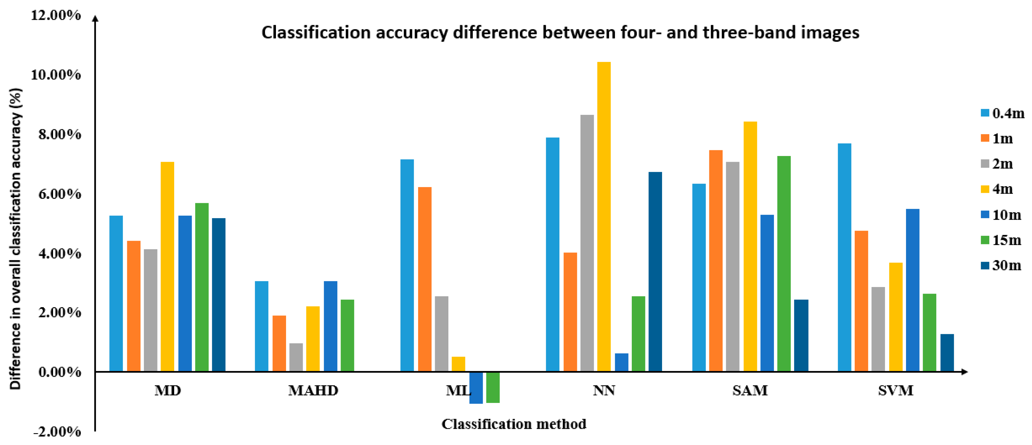
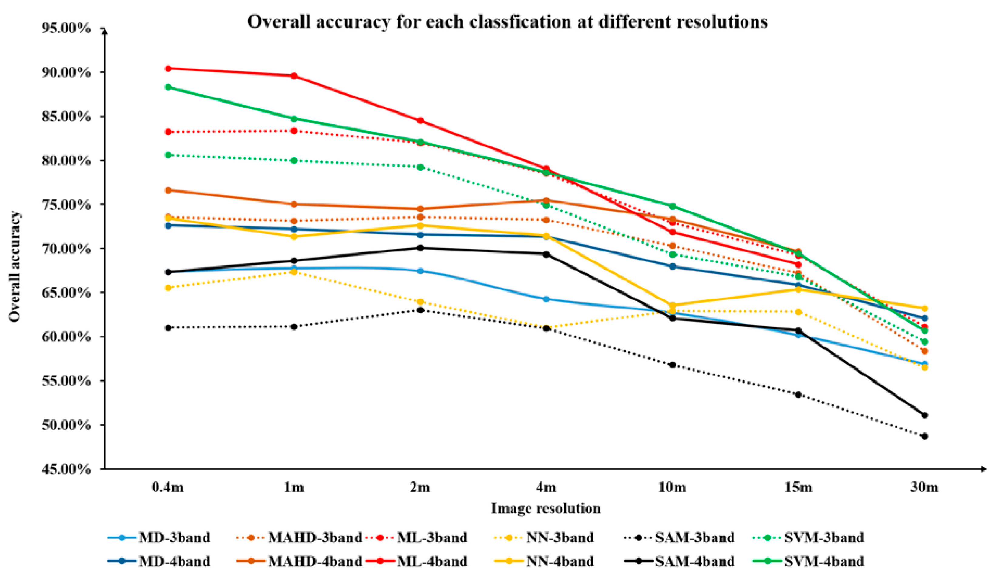
| Resolution (m) | 1 MD | MAHD | ML | NN | SAM | SVM | ||||||
|---|---|---|---|---|---|---|---|---|---|---|---|---|
| Three-Band | Four-Band | Three-Band | Four-Band | Three-Band | Four-Band | Three-Band | Four-Band | Three-Band | Four-Band | Three-Band | Four-Band | |
| 0.4 | 67.37 | 72.63 | 73.58 | 76.63 | 83.26 | 90.42 | 65.58 | 73.47 | 61.05 | 67.37 | 80.63 | 88.32 |
| 1 | 67.79 | 72.21 | 73.16 | 75.05 | 83.37 | 89.58 | 67.37 | 71.37 | 61.16 | 68.63 | 80.00 | 84.74 |
| 2 | 67.47 | 71.58 | 73.58 | 74.53 | 82.00 | 84.53 | 64.00 | 72.63 | 63.05 | 70.11 | 79.26 | 82.11 |
| 4 | 64.32 | 71.37 | 73.26 | 75.47 | 78.53 | 79.05 | 61.05 | 71.47 | 60.95 | 69.37 | 74.95 | 78.63 |
| 10 | 62.74 | 68.00 | 70.32 | 73.37 | 72.95 | 71.89 | 62.95 | 63.58 | 56.84 | 62.11 | 69.37 | 74.84 |
| 15 | 60.21 | 65.89 | 67.26 | 69.68 | 69.26 | 68.21 | 62.84 | 65.37 | 53.47 | 60.74 | 66.84 | 69.47 |
| 30 | 56.95 | 62.11 | 58.42 | - | 61.16 | - | 56.53 | 63.26 | 48.74 | 51.16 | 59.47 | 60.74 |
| is the best result for the four-band images at the same resolution. | is the best result for the three-band RGB images at the same resolution. | ||
| is the poorest result for the four-band images at the same resolution. | is the poorest result for the three-band RGB images at the same resolution. |
| Resolution (m) | 1 MD | MAHD | ML | NN | SAM | SVM | ||||||
|---|---|---|---|---|---|---|---|---|---|---|---|---|
| Three-Band | Four-Band | Three-Band | Four-Band | Three-Band | Four-Band | Three-Band | Four-Band | Three-Band | Four-Band | Three-Band | Four-Band | |
| 0.4 | 0.593 | 0.660 | 0.673 | 0.711 | 0.792 | 0.881 | 0.565 | 0.664 | 0.515 | 0.598 | 0.759 | 0.866 |
| 1 | 0.597 | 0.655 | 0.669 | 0.692 | 0.792 | 0.870 | 0.586 | 0.636 | 0.515 | 0.614 | 0.751 | 0.809 |
| 2 | 0.592 | 0.648 | 0.673 | 0.685 | 0.774 | 0.805 | 0.540 | 0.652 | 0.536 | 0.631 | 0.740 | 0.776 |
| 4 | 0.551 | 0.645 | 0.669 | 0.697 | 0.730 | 0.736 | 0.505 | 0.539 | 0.508 | 0.621 | 0.685 | 0.732 |
| 10 | 0.534 | 0.600 | 0.631 | 0.670 | 0.659 | 0.644 | 0.522 | 0.537 | 0.454 | 0.527 | 0.615 | 0.685 |
| 15 | 0.500 | 0.575 | 0.594 | 0.623 | 0.613 | 0.598 | 0.532 | 0.562 | 0.415 | 0.508 | 0.581 | 0.617 |
| 30 | 0.460 | 0.527 | 0.482 | - | 0.511 | - | 0.448 | 0.536 | 0.349 | 0.383 | 0.486 | 0.504 |
| is the best result for the four-band images at the same resolution. | is the best result for the three-band RGB images at the same resolution. | ||
| is the poorest result for the four-band images at the same resolution. | is the poorest result for the three-band RGB images at the same resolution. |
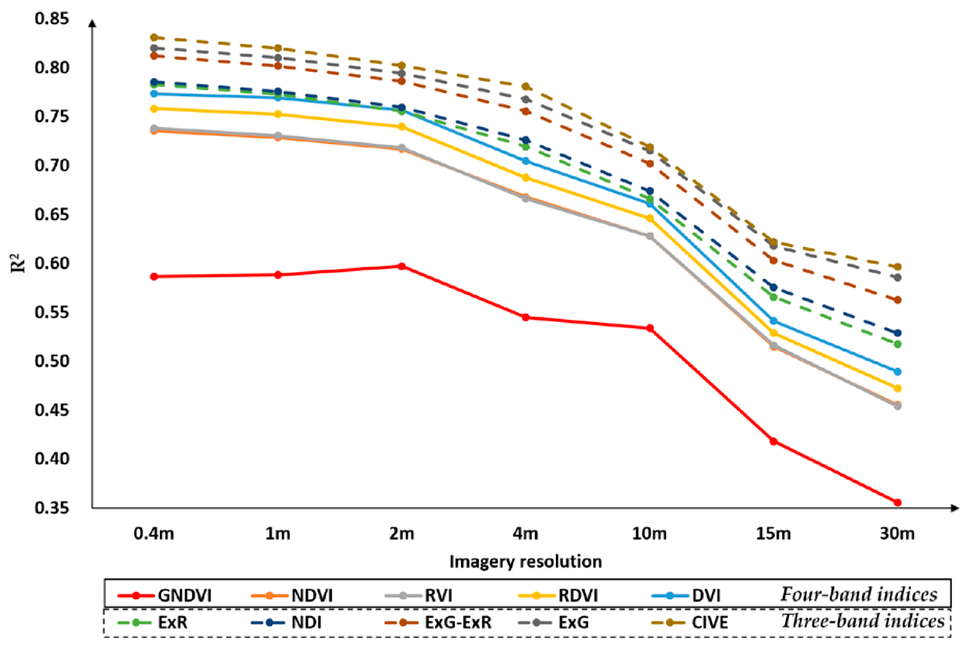
| Resolutions (m) | Second-Degree Regression Model | R2 | RMSE | Second-Degree Regression Model | R2 | RMSE | ||
|---|---|---|---|---|---|---|---|---|
| 0.4 | y = –3.136x2 + 12.260x + 0.343 | 0.735 | 0.869 | y = –28.026x2 + 22.164x + 2.199 | 0.786 | 0.782 | ||
| 1 | y = –4.261x2 + 12.781x + 0.322 | 0.729 | 0.880 | y = –29.984x2 + 22.380x + 2.217 | 0.776 | 0.800 | ||
| 2 | y = –2.288x2 + 11.339x + 0.543 | 0.717 | 0.899 | y = –29.172x2 + 21.984x + 2.234 | 0.760 | 0.828 | ||
| 4 | NDVI | y = 0.482x2 + 9.429x + 0.797 | 0.668 | 0.974 | NDI | y = –26.863x2 + 21.414x + 2.245 | 0.726 | 0.884 |
| 10 | y = 2.315x2 + 8.396x + 0.929 | 0.628 | 1.030 | y = –25.644x2 + 20.953x + 2.291 | 0.674 | 0.964 | ||
| 15 | y = 2.864x2 + 7.455x + 1.209 | 0.515 | 1.177 | y = –29.336x2 + 20.953x + 2.398 | 0.575 | 1.101 | ||
| 30 | y = 3.309x2 + 7.462x + 1.375 | 0.455 | 1.247 | y = –33.347x2 + 22.199x + 2.530 | 0.529 | 1.160 | ||
| 0.4 | y = –0.985x2 + 6.500x – 4.911 | 0.738 | 0.864 | y = 7.160x2 + 18.325x + 1.934 | 0.820 | 0.716 | ||
| 1 | y = –1.036x2 + 6.671x – 5.021 | 0.730 | 0.877 | y = 4.397x2 + 18.705x + 1.943 | 0.810 | 0.736 | ||
| 2 | y = –0.914x2 + 6.100x – 4.418 | 0.718 | 0.897 | y = –2.358x2 + 19.773x + 1.946 | 0.794 | 0.766 | ||
| 4 | RVI | y = –0.669x2 + 5.006x – 3.340 | 0.666 | 0.976 | ExG | y = –9.882x2 + 21.319x + 1.930 | 0.768 | 0.814 |
| 10 | y = –0.639x2 + 4.886x – 3.210 | 0.628 | 1.030 | y = –17.495x2 + 22.580x + 1.963 | 0.715 | 0.903 | ||
| 15 | y = –0.62412 + 4.690x – 2.824 | 0.516 | 1.175 | y = –35.471x2 + 25.053x + 2.036 | 0.618 | 1.044 | ||
| 30 | y = –0.425x2 + 3.938x – 1.984 | 0.454 | 1.248 | y = –46.548x2 + 27.938x + 2.117 | 0.586 | 1.088 | ||
| 0.4 | y = 1.224x2 + 14.486x + 0.434 | 0.774 | 0.804 | y = –40.893x2 – 16.067x + 5.118 | 0.783 | 0.787 | ||
| 1 | y = –1.483x2 + 15.479x + 0.385 | 0.769 | 0.811 | y = –44.037x2 – 15.498x + 5.117 | 0.773 | 0.805 | ||
| 2 | y = 1.093x2 + 14.018x + 0.561 | 0.756 | 0.34 | y = –42.559x2 – 15.349x + 5.089 | 0.755 | 0.835 | ||
| 4 | DVI | y = 3.284x2 + 12.800x + 0.700 | 0.705 | 0.918 | ExR | y = –38.091x2 – 15.661x + 5.064 | 0.719 | 0.895 |
| 10 | y = 4.972x2 + 12.151x + 0.768 | 0.661 | 0.984 | y = –34.933x2 – 15.725x + 5.061 | 0.666 | 0.976 | ||
| 15 | y = 1.844x2 + 12.531x + 0.922 | 0.541 | 1.144 | y = –39.279x2 – 14.288x + 5.057 | 0.566 | 1.113 | ||
| 30 | y = 1.155x2 + 13.080x + 1.024 | 0.489 | 1.207 | y = –43.991x2 – 14.311x + 5.280 | 0.518 | 1.173 | ||
| 0.4 | GNDVI | y = 17.322x2 + 12.225x − 0.058 | 0.587 | 1.086 | ExG-ExR | y = –3.772x2 + 10.486 x + 3.512 | 0.812 | 0.732 |
| 1 | y = 10.846x2 + 14.749x − 0.257 | 0.588 | 1.084 | y = –4.507x2 + 10.447x + 3.535 | 0.802 | 0.752 | ||
| 2 | y = 22.313x2 + 9.590x + 0.295 | 0.597 | 1.072 | y = –5.302x2 + 10.386x + 3.555 | 0.786 | 0.781 | ||
| 4 | y = 36.054x2 + 2.922x + 1.015 | 0.545 | 1.140 | y = –6.276x2 + 10.450x + 3.584 | 0.755 | 0.835 | ||
| 10 | y = 48.872x2 – 1.945x + 1.441 | 0.534 | 1.153 | y = –7.132x2 + 10.403x + 3.637 | 0.702 | 0.922 | ||
| 15 | y = 47.662x2 – 2.728x + 1.753 | 0.418 | 1.289 | y = –10.209x2 + 10.191x + 3.761 | 0.603 | 1.064 | ||
| 30 | y = 64.286x2 – 8.581x + 2.413 | 0.356 | 1.356 | y = –12.854x2 + 10.706x + 3.991 | 0.563 | 1.117 | ||
| 0.4 | y = –2.997x2 + 14.125x + 0.298 | 0.758 | 0.831 | y = 384.199x2 – 14,479.250x + 136,420.264 | 0.831 | 0.694 | ||
| 1 | y = –4.851x2 + 14.900x + 0.259 | 0.752 | 0.841 | y = 319.268x2 – 12,042.058x + 113,550.278 | 0.820 | 0.717 | ||
| 2 | y = –2.690x2 + 13.499x + 0.452 | 0.740 | 0.862 | y = 235.416x2 – 8894.888x + 84,020.097 | 0.802 | 0.751 | ||
| 4 | RDVI | y = 0.794x2 + 11.425x + 0.696 | 0.688 | 0.944 | CIVE | y = 213.405x2 – 8070.489x + 76,300.729 | 0.781 | 0.791 |
| 10 | y = 2.901x2 + 10.422x + 0.809 | 0.646 | 1.005 | y = 101.976x2 – 3888.242x + 37,058.058 | 0.719 | 0.895 | ||
| 15 | y = 1.439x2 + 10.415x + 0.984 | 0.529 | 1.159 | y = –99.169x2 + 3663.297x – 33,818.112 | 0.622 | 1.039 | ||
| 30 | y = 2.492x2 + 10.099x + 1.183 | 0.472 | 1.227 | y = –174.059x2 + 6471.318x – 60,139.730 | 0.596 | 1.073 |
| is the best results at the same VI | is the second result at the same VI | is the third result at the same VI |
© 2017 by the authors. Licensee MDPI, Basel, Switzerland. This article is an open access article distributed under the terms and conditions of the Creative Commons Attribution (CC BY) license (http://creativecommons.org/licenses/by/4.0/).
Share and Cite
Zhang, J.; Yang, C.; Zhao, B.; Song, H.; Clint Hoffmann, W.; Shi, Y.; Zhang, D.; Zhang, G. Crop Classification and LAI Estimation Using Original and Resolution-Reduced Images from Two Consumer-Grade Cameras. Remote Sens. 2017, 9, 1054. https://doi.org/10.3390/rs9101054
Zhang J, Yang C, Zhao B, Song H, Clint Hoffmann W, Shi Y, Zhang D, Zhang G. Crop Classification and LAI Estimation Using Original and Resolution-Reduced Images from Two Consumer-Grade Cameras. Remote Sensing. 2017; 9(10):1054. https://doi.org/10.3390/rs9101054
Chicago/Turabian StyleZhang, Jian, Chenghai Yang, Biquan Zhao, Huaibo Song, Wesley Clint Hoffmann, Yeyin Shi, Dongyan Zhang, and Guozhong Zhang. 2017. "Crop Classification and LAI Estimation Using Original and Resolution-Reduced Images from Two Consumer-Grade Cameras" Remote Sensing 9, no. 10: 1054. https://doi.org/10.3390/rs9101054