Article

Generative Adversarial Networks-Based Semi-Supervised Learning for Hyperspectral Image Classification

Guangdong Provincial Key Laboratory of Urbanization and Geo-Simulation, Center of Integrated Geographic Information Analysis, School of Geography and Planning, Sun Yat-Sen University, Guangzhou 510275, China
*
Author to whom correspondence should be addressed.
Remote Sens. 2017, 9(10), 1042; https://doi.org/10.3390/rs9101042
Submission received: 31 August 2017 / Revised: 5 October 2017 / Accepted: 10 October 2017 / Published: 12 October 2017

Abstract

:
Classification of hyperspectral image (HSI) is an important research topic in the remote sensing community. Significant efforts (e.g., deep learning) have been concentrated on this task. However, it is still an open issue to classify the high-dimensional HSI with a limited number of training samples. In this paper, we propose a semi-supervised HSI classification method inspired by the generative adversarial networks (GANs). Unlike the supervised methods, the proposed HSI classification method is semi-supervised, which can make full use of the limited labeled samples as well as the sufficient unlabeled samples. Core ideas of the proposed method are twofold. First, the three-dimensional bilateral filter (3DBF) is adopted to extract the spectral-spatial features by naturally treating the HSI as a volumetric dataset. The spatial information is integrated into the extracted features by 3DBF, which is propitious to the subsequent classification step. Second, GANs are trained on the spectral-spatial features for semi-supervised learning. A GAN contains two neural networks (i.e., generator and discriminator) trained in opposition to one another. The semi-supervised learning is achieved by adding samples from the generator to the features and increasing the dimension of the classifier output. Experimental results obtained on three benchmark HSI datasets have confirmed the effectiveness of the proposed method, especially with a limited number of labeled samples.

1. Introduction

A hyperspectral image [1,2,3,4] contains hundreds of continuous narrow spectral bands, spanning the visible to infrared spectrum. Hyperspectral sensors have attracted much interest in remote sensing for providing abundant and valuable information over the last few decades. With the useful information, HSI has played a vital role in many applications, among which classification [5,6,7] is one of the crucial processing steps that has received enormous attention. The foremost task in hyperspectral classification is to train an effective classifier with the given training set from each class. Therefore, sufficient training samples are crucial to train a reliable classifier. However, in reality, it is time-consuming and expensive to obtain a large number of samples with class labels. This difficulty will result in the curse of dimensionality (i.e., Hughes phenomenon) and will induce the risk of overfitting.
Much work has been carried out to design suitable classifiers to deal with the above-mentioned problems in the last decades. In general, those methods can be categorized into three types, i.e., unsupervised, supervised and semi-supervised methods. Unsupervised methods focus on training models from large unlabeled samples. Since no labeled samples are required, the unsupervised methods can be easily applied in the hyperspectral processing area. Many unsupervised methods, such as fuzzy clustering [8], fuzzy C-Means method [9], artificial immune algorithm [10], graph-based method [11], have demonstrated impressive results in hyperspectral classification. However, one cannot ensure the relationship between clusters and classes with too little priori knowledge.
Supervised classifiers, which are widely used in hyperspectral classification, can yield improved performance by utilizing the priori information of the class labels. Typical supervised classifiers include the support vector machine (SVM) [12,13], artificial neural networks (ANN) [14] and sparse representation-based classification (SRC) [15,16], etc. SVM is a kind of kernel-based method that aims at exploring the optimal separating hyperplane between different classes, ANN is motivated by the biological learning process of human brain, while SRC stems from the rapid development of compressed sensing in recent years. Versatile as the supervised classifiers are, their performance heavily depends on the number of labeled samples. In contrast to the urgent needs of labeled samples, they ignore the large number of unlabeled samples to assist classification.
Semi-supervised learning is designed to alleviate the “small-sample problem” by utilizing both the limited labeled samples and the wealth of unlabeled samples that can be easily obtained without significant cost. The semi-supervised methods can be roughly divided into four types: (1) generative models [17,18], which estimate the conditional density to obtain the labels of unlabeled samples. (2) Low density separation, which aims to place boundaries in regions where few samples (labeled or unlabeled) existed. One of the state-of-the-art algorithms is the transductive support vector machine (TSVM) [19,20,21]. (3) Graph-based methods [22,23,24,25,26] that utilize labeled and unlabeled samples to construct graphs and minimize the energy function, and thus, assigning labels to unlabeled samples. (4) Wrapper-based methods, which apply a supervised learning method iteratively and a certain amount of unlabeled samples are labeled in each iteration. The self-training [27,28] and co-training [29,30] algorithms are commonly-used wrapper-based methods.
Notably that the samples within a small neighborhood are likely to belong to the same class and thus, the spatial correlation between neighboring samples can be incorporated into the classification to further improve the performance of the classifiers. For instance, the spatial contextual information [31,32,33,34,35,36,37,38,39] can be extracted by various spatial filters. Segmentation methods (e.g., watershed segmentation [40] and superpixel segmentation [41,42]) can also be adopted to exploit the spatial homogeneity of the HSI. One can also use the spatial similarity of neighboring samples [43,44,45] in the classification stages. Regularizations [15,46,47,48,49,50,51,52,53] can be added in the classifiers to refine the classification performance. Different from the above-mentioned vector/matrix-based methods, there are some three-dimension (3D)/tensor-based methods [34,54,55,56,57] that respect the 3D nature of the HSI and process the 3D cube as a whole entity. The 3D/tensor-based methods have demonstrated considerable improvement since the joint spectral-spatial structure information is effectively exploited.
However, most of the aforementioned methods can only extract features of the original HSI dataset in a shallow manner. Deep learning [58], which can hierarchically obtain the high-level abstract representation, has recently become a hotspot in the image processing area, especially in hyperspectral classification. Typical deep architectures involve the stacked autoencoder (SAE) [59], deep brief network (DBN) [60] and convolutional neural networks (CNN) [61]. The above-mentioned classification frameworks are supervised, which require a large number of labeled samples for training. Recently, a semi-supervised classifier based on multi-decision labeling and contextual deep learning (i.e., CDL-MD-L) is proposed by [62], which has demonstrated promising results in hyperspectral classification.
In this paper, a generative adversarial networks (GANs)-based semi-supervised method is proposed for hyperspectral classification. To extract the spectral-spatial features, we extend the existing two-dimensional bilateral filter (2DBF) [36,63,64] into its three-dimensional version (i.e., 3DBF), which is a non-iterative method for nonlinear and edge-preserving smoothing. The 3DBF is suitable for spectral-spatial feature extraction since it respects the 3D nature of the HSI cube. Subsequently, the outputs of the previous step can be utilized to train GANs [65,66], which are promising neural networks that have been the focus of attention in recent years. In this paper, the GANs are trained for semi-supervised classification of HSI to use the limited labeled samples and vast of unlabeled samples. The semi-supervised learning is performed by adding samples from the generators to the extracted features and increasing the dimension of the classifier output.
Compared to the existing literature, the contribution of this paper lies in two aspects:
  • We extract the spectral-spatial features by the 3DBF. Compared to the vector/matrix-based methods, the structural features extracted by the 3DBF can effectively preserve the spectral-spatial information by naturally obeying the 3D form of the HSI and treating the 3D cube as a whole entity.
  • We classify the HSI in a semi-supervised manner by the GANs. Compared to the supervised methods, the GANs can utilize both limited training samples and abundant of unlabeled samples. Compared to the non-adversarial networks, the GANs take advantage of the discriminative models to train the generative network based on game theory.
The remaining part of this paper is organized as follows. Section 2 describes the proposed semi-supervised classification method in detail. Section 3 reports the experimental results and analyses on three benchmark HSI datasets. Finally, discussions and conclusions are drawn in Section 4 and Section 5.

2. Proposed Semi-Supervised Method

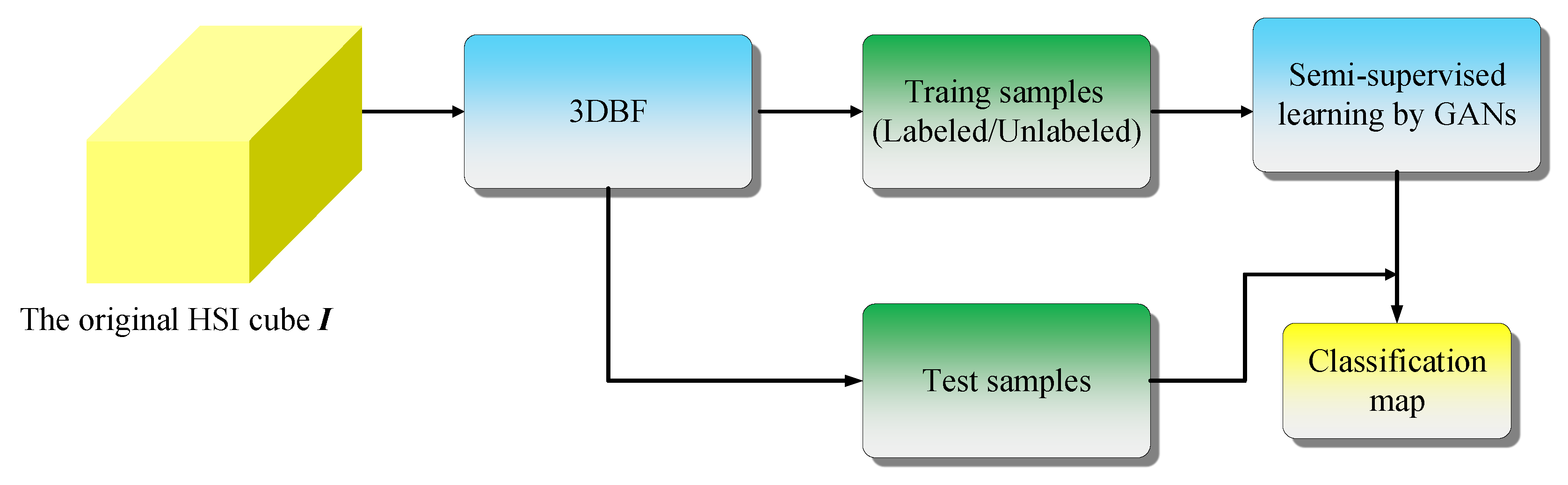
The conceptual framework of the proposed method is shown in Figure 1, which is composed of two parts: (1) feature extraction; (2) semi-supervised learning. The spectral-spatial features of the original HSI cube I can be extracted by the 3DBF, which is a 3D filter that can obey the 3D nature of the HSI and extract the spectral-spatial features simultaneously. Subsequently, GANs are utilized in the feature space for semi-supervised classification by taking full advantage of both the limited labeled samples and the sufficient unlabeled samples. The classification map can be achieved by visualizing the classification results of different samples.
It is noteworthy that both 3DBF and GANs are of great importance for semi-supervised learning of HSI classification. On the one hand, 3DBF is adopted for extracting the spectral-spatial features of the HSI. As emphasized in Section 1, incorporating spatial information into the hyperspectral classification helps to improve the performance the classifiers, and thus, exploring spectral-spatial feature extraction methods has become an important research topic in the hyperspectral community. In addition, since the HSI data is naturally a 3D cube, the 3D/tensor-based methods are more effective to extract the joint spectral-spatial structure information than the vector/matrix-based methods. As will be shown in Section 3.3, the GANs with the original spectral features (i.e., Spec-GANs) provide much worse performance than the GANs with 3DBF features (i.e., 3DBF-GANs), which further highlights the significance of the 3DBF. On the other hand, GANs are utilized for semi-supervised classification of the HSI. The recent development of deep learning has opened up new opportunities for hyperspectral classification. GANs, which are newly proposed deep architectures for training deep generative models by a minimax game, have shown promising results in unsupervised/semi-supervised learning. Although the GANs have been successfully employed in various areas and demonstrated remarkable success, the application of GANs in semi-supervised hyperspectral classification has never been addressed in the literature to the best of our knowledge. Therefore, it is valuable for us to represent the first attempt to develop a semi-supervised hyperspectral classification framework based on GANs. In this section, we introduce the detailed procedure of the proposed semi-supervised classification method, elaborating on the spectral-spatial feature extraction based on 3DBF and semi-supervised classification of HSI by GANs.

2.1. Spectral-Spatial Features Extracted by 3D Bilateral Filter

The bilateral filter was originally introduced by [63] under the name “SUSAN”. It was then rediscovered by [67] termed as “bilateral filter”, which is now the widely used name in the literature. Over the past few years, the bilateral filter has emerged as a powerful tool for several applications, such as image denoising [64] and hyperspectral classification [36]. The great success of the bilateral filter stems from several properties. It is a local, non-iterative and simple filter, which smooths images while preserving edges in terms of a nonlinear combination of the neighboring pixels. Although the bilateral filter has announced impressive results in hyperspectral classification, it is performed in each two-dimensional probability map, and thus ignoring the 3D nature of the HSI cube.
In this paper, we extend the bilateral filter to 3DBF for spectral-spatial feature extraction of the HSI volumetric data. Suppose the original HSI cube can be represented as I R m × n × b , where m , n and b indicate the number of rows, columns and spectral bands, respectively, the result I b f of the 3DBF, which replaces each pixel in the I by a weighted average of its neighbors, can be defined by
I b f ( p ) = 1 W b f ( p ) q S G σ s ( p q ) G σ r ( | I ( p ) I ( q ) | ) I ( q )
with
W b f ( p ) = q S G σ s ( p q ) G σ r ( | I ( p ) I ( q ) | )
where p refers to the coordinate of the HSI cube I , i.e., p = ( x , y , z ) , x = 1 , , m , y = 1 , 2 , , n , z = 1 , 2 , , b , q indicates the index of the neighborhoods centered at p , W b f denotes the normalizing term of the neighborhood pixels q , G σ s ( p q ) = exp ( p q 2 / 2 σ s 2 ) and G σ r ( | I ( p ) I ( q ) | ) = exp ( | I ( p ) I ( q ) | 2 / 2 σ r 2 ) are the Gaussian filters measuring the distance in the 3D image domain (i.e., the spectral-spatial domain S ) and the distance on the intensity axis (i.e., the range domain R ), respectively.
To speed up the implementation, we decompose the 3DBF into a convolution followed by two nonlinearities based on signal processing grounds. Note that the nonlinearity of the 3DBF (see Equation (1)) originates from the division by W b f and the dependency on the intensities by G σ r ( | I ( p ) I ( q ) | ) , we study each point separately and isolate them during computation. Multiplying both sides of Equation (1) by W b f , Equations (1) and (2) can be rewritten as
W b f ( p ) I b f ( p ) W b f ( p ) = q S G σ s ( p q ) G σ r ( | I ( p ) I ( q ) | ) I ( q ) 1
We then define a function W whose value is 1 everywhere ( W is a function whose value is 1 everywhere, i.e., W ( ( x , y , z ) ) = 1 , x = 1 , , m , y = 1 , 2 , , n , z = 1 , 2 , , b . Therefore, the size of W is the same as that of the original HSI cube) to maintain the weighted mean property of the 3DBF and represent Equation (3) as
W b f ( p ) I b f ( p ) W b f ( p ) = q S G σ s ( p q ) G σ r ( | I ( p ) I ( q ) | ) W ( q ) I ( q ) W ( q )
The above-mentioned Equation (4) can be equivalently expressed as
W b f ( p ) I b f ( p ) W b f ( p ) = q S ζ R G σ s ( p q ) G σ r ( | I ( p ) ζ | ) δ ( ζ I ( q ) ) W ( q ) I ( q ) W ( q )
where R denotes the intensity interval, δ ( ζ ) is the Kronecker symbol with δ ( ζ ) = 1 if ζ = 0 , and δ = 0 otherwise. Specifically, δ ( ζ I ( q ) ) = 1 if and only if ζ = I ( q ) . The sum in Equation (5) is over the product space S × R , on which we express the functions by lowercases. That means, g δ s , δ r represents a Gaussian kernel given by
g δ s , δ r : ( x S , ζ R ) G δ s ( x ) G δ r ( | ζ | )
Based on Equation (5), two functions i and w can be build on S × R by
i : ( x S , ζ R ) I ( x )
and
w : ( x S , ζ R ) δ ( ζ I ( x ) ) W ( x )
Observed from the definitions of i and w in Equations (7) and (8), we have
I ( x ) = i ( x , I ( x ) )
W ( x ) = w ( x , I ( x ) )
w ( x , ζ ) = 0 , ζ I ( x )
Let the input of g δ s , δ r be ( p q , I ( p ) ζ ) , the input of i and w be ( q , ζ ) , Equation (5) becomes
W b f ( p ) I b f ( p ) W b f ( p ) = ( q , ζ ) S × R g δ s , δ r ( p q , I ( p ) ζ ) w ( q , ζ ) i ( q , ζ ) w ( q , ζ ) = g δ s , δ r w i w ( p , I ( p ) )
where “⊗” indicates the convolution operator.
Therefore, the 3DBF can be modeled by
I b f ( p ) = w b f ( p , I ( p ) ) i b f ( p , I ( p ) ) w b f ( p , I ( p ) )
where the functions w b f and i b f are defined as ( w b f i b f , w b f ) = g δ s , δ r ( w i , w ) .
In hyperspectral analysis, the 3D image domain (i.e., the spectral-spatial domain S ) is a x y z volume and the range domain R is a simple axis labelled ζ . As described in Equation (
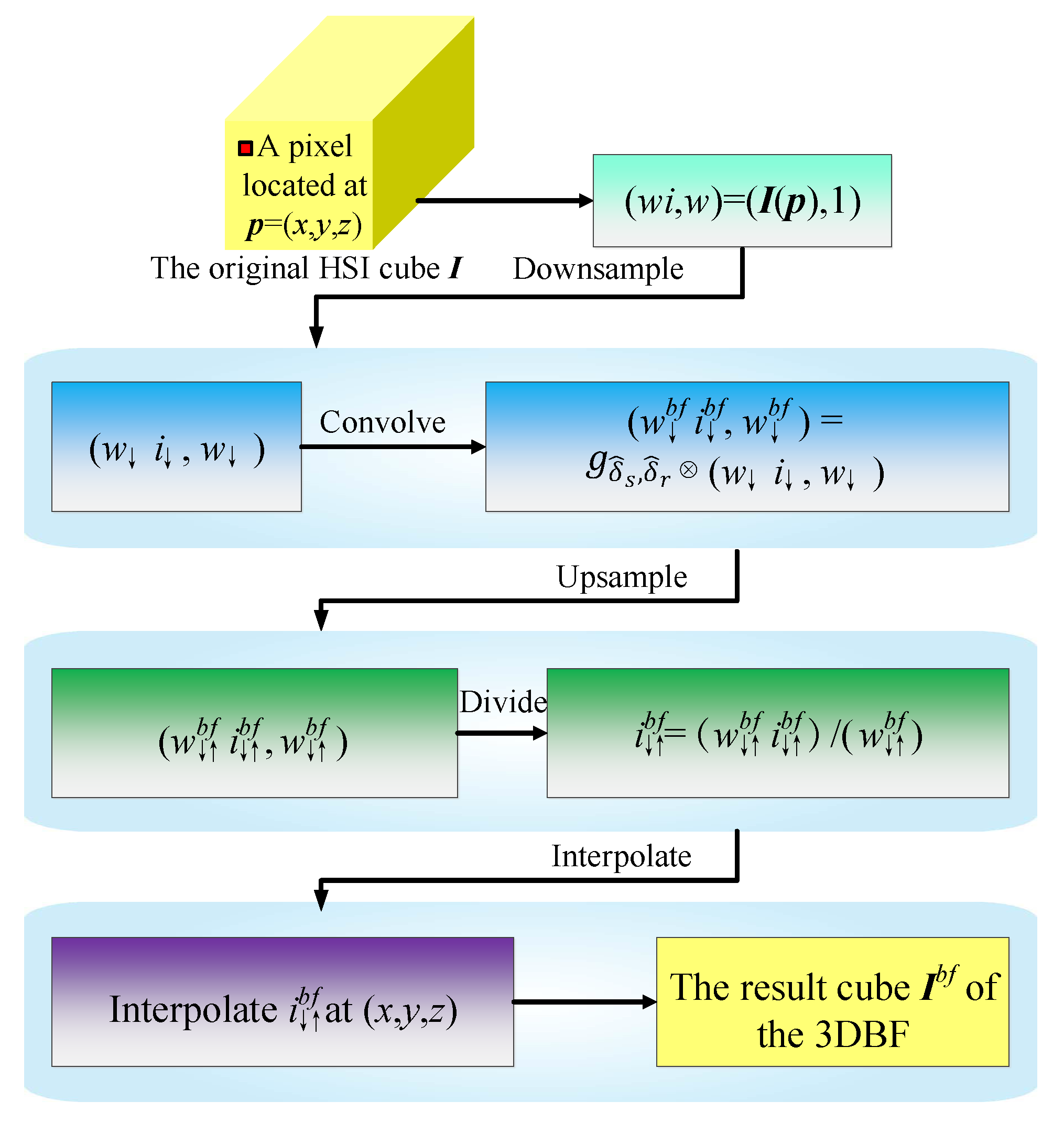
13), the 3DBF can be achieved by the following three steps:
  • Convolve w i and w with a Gaussian defined on x y z ζ . In this step, w i and w are “blurred” into w b f ( x , y , z , ζ ) i b f ( x , y , z , ζ ) and w b f ( x , y , z , ζ ) , respectively.
  • Obtain i b f ( x , y , z , ζ ) by dividing w b f ( x , y , z , ζ ) i b f ( x , y , z , ζ ) by w b f ( x , y , z , ζ ) ;
  • Compute the value of i b f at ( x , y , z , ζ ) to get the filtered result I b f ( x , y , z ) .
Moreover, the 3DBF can be accelerated by downsample and upsample without changing the major steps of the implementation. That is, we downsample ( w i , w ) to obtain ( w i , w ) , perform the convolution to generate ( w b f i b f , w ) b f , followed by upsample ( w b f i b f , w b f ) to get ( w b f i b f , w b f ) . The remaining steps are the same as the above-mentioned steps 2 and 3. To sum up, the schematic diagram of the 3DBF can be depicted in Figure 2, by which the original HSI cube I is filtered and the spectral-spatial feature cube I b f is obtained. It is worth underlining that the dimension of the 3DBF cube I b f is the same as that of the original HSI cube, i.e., I b f R m × n × b . As will be shown in Figures 9 and 10, the spectral and spatial profiles of the 3DBF smooth the original data while still preserving edges.

2.2. Semi-Supervised Classification of HSI by Generative Adversarial Networks

2.2.1. Brief of Generative Adversarial Networks

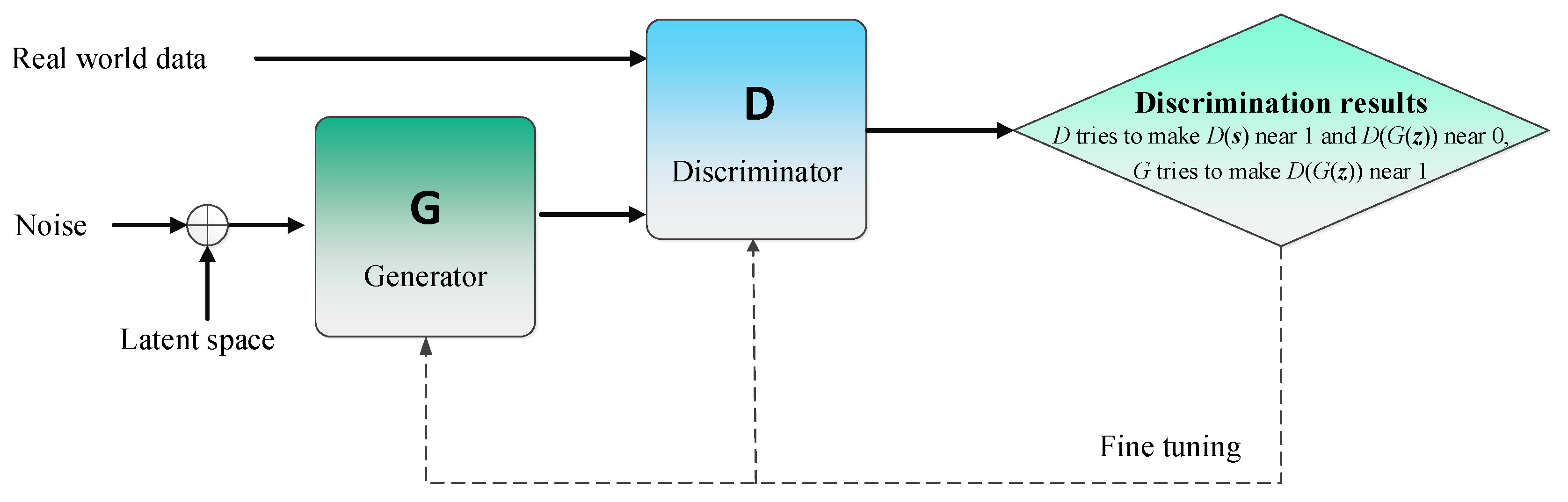
GANs are newly proposed deep architectures based on adversarial nets to train the model in an adversarial fashion to generate data mimicking certain distributions. Unlike the other deep learning methods, a GAN is an architecture around two functions (see Figure 3), i.e., a generator G, which can map a sample from a random uniform distribution to the data distribution, and a discriminator D, which is trained to distinguish whether a sample belongs to the real data distribution. In GANs, the generator and discriminator are learned jointly based on game theory. The generator G and the discriminator D can be trained in an alternating manner. In each step, G produces a sample from the random noise z that may fool D, and D is then presented the real data samples as well as the samples generated by G to classify the samples as “real” or “fake”. Subsequently, G is rewarded for producing samples that can “fool” D and D for correct classification. Both functions are updated and the iteration stops until a Nash equilibrium is achieved. In greater detail, let D ( s ) be the probability that s comes from the real data rather than the generator, G and D play a minimax game with the following value function
min G max D V ( D , G ) = E s p data ( s ) [ log D ( s ) ] + E z p z ( z ) [ log ( 1 D ( G ( z ) ) ) ]
Much work has been carried out to improve the GAN since it was pioneered by Goodfellow et al. [65] in 2014. Two remarkable aspects can be highlighted: theory and application. On the one hand, several improved versions of GANs in aspects of stability of training, perceptual quality, etc., have been proposed in recent literature, including the well-known deep convolutional GAN (DC-GAN) [68], conditional GAN (C-GAN) [69], Laplacian pyramid GAN (LAP-GAN) [70], information-theoretic extension to the GAN (Info-GAN) [71], unrolled GAN [72] and Wasserstein GAN (W-GAN) [73]. On the other hand, recent work has also shown that GANs can provide very successful results in image generation [74], image super resolution [75], image inpainting [76] and semi-supervised learning [77].

2.2.2. Generative Adversarial Networks for Classification

GANs, which can train deep generative models with a minimax game, have recently emerged as powerful tools for unsupervised and semi-supervised classification. Several unsupervised/ semi-supervised techniques motivated by the GANs have sprung up over the past few years to overcome the difficulties of labeling large amounts of training samples. For instance, DC-GAN is proposed in [68] to bridge the gap between the success of the CNN for supervised and unsupervised learning. Several constraints are evaluated to make the convolutional GANs stable to train, and the trained discriminators are applied for image classification tasks, resulting in competitive performance with other unsupervised methods. Info-GAN is proposed in [71] to learn disentangled representations in a completely unsupervised manner. As an information-theoretic extension to the GAN, the Info-GAN maximizes the mutual information between a small subset of the latent variables and the observation, and therefore, interpretable and disentangled representations can be learned. Categorical GAN (CatGAN) [77], which is a framework for robust unsupervised and semi-supervised learning, combines ANN classifiers with an adversarial generative model that regularizes a discriminatively trained classifier. By heuristically understanding the non-convergence problem, an improved semi-supervised learning method is proposed in [66], which can be regarded as a continuation and refinement of the effort in [77]. Moreover, Premachandran and Yuille [78] learns a deep network by generative adversarial training. Features learned by adversarial training is fused with a traditional unsupervised classification approach, i.e., k-means clustering, and the combination produces better results than direct prediction. In situation of semi-supervised classification, the adversarial training has the potential to outperform supervised learning.
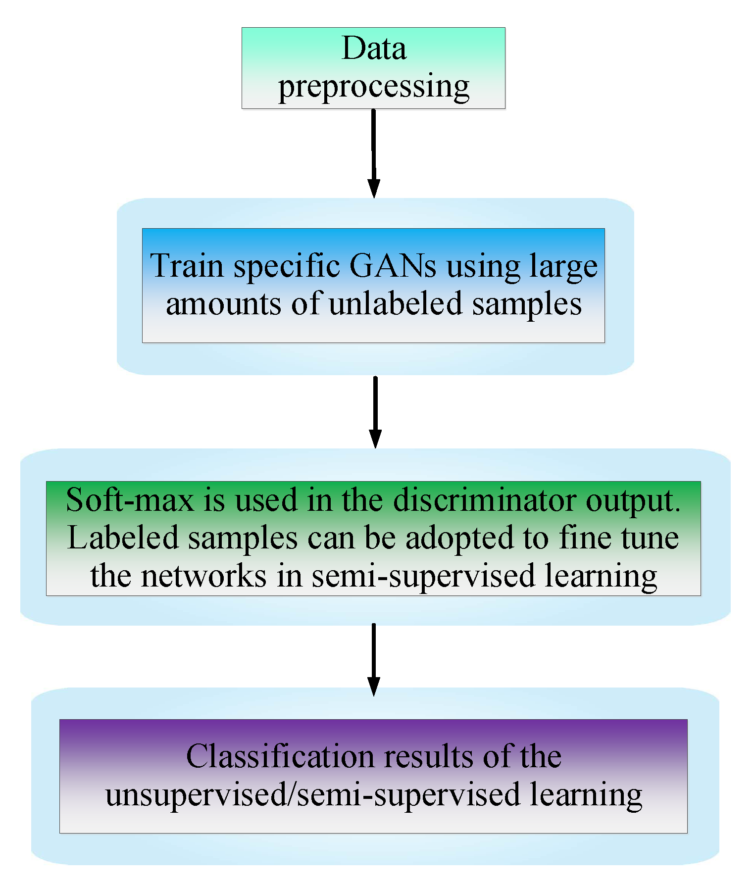
Note that different versions of GANs have different objective functions and procedures, it is hard to obtain a unified architecture for describing the unsupervised/semi-supervised techniques. In this section, we try to give a schematic illustration of the procedure for unsupervised/semi-supervised learning in Figure 4, which contains the main steps in most of the scenarios but not all of them. It is noteworthy that the logistic regression classifier based on the soft-max function is employed to discriminate different classes in Figure 4. That means, by applying the soft-max function, the class probabilities of s can be expressed as
p model ( c = j | s ) = exp ( l j ) c = 1 C exp ( l c ) , j = 1 , 2 , , C
and the class label of s can be determined by
class ( s ) = arg max j p model ( c = j | s )
In addition, despite remarkable success of GANs, their applications in semi-supervised classification of HSI are surprisingly unstudied to the best of our knowledge. Therefore, this study represents the first attempt to develop a semi-supervised classification framework for the HSI.

2.2.3. Hyperspectral Classification Framework Using Generative Adversarial Networks

In hyperspectral classification, a standard classifier assigns each sample s to one of the C possible classes based on the training samples available for each class. For instance, a logistic regression classifier takes s as input and outputs a C-dimensional vector, which can be turned into the class probabilities by soft-max p model ( c = j | s ) = exp ( l j ) c = 1 C exp ( l c ) . Classifiers like this usually have a cross-entropy objective function in supervised scenario. That means, a discriminative model can be trained by minimizing the objective function between observed labels and the model predictive distribution p model ( c | s ) . However, the supervised learning usually needs enough labeled training samples to guarantee the representativeness and prevent the classifier from overfitting, especially for a deep discriminative model with huge parameter volume such as CNN. The strong demand for abundant training samples conflicts with the fact that the labels of the samples are extremely difficult and expensive to identify. At the same time, there are vast of unlabeled samples in the HSI. Therefore, we propose a GANs-based classification method [65,66] to simultaneously utilize both the limited labeled samples and the sufficient unlabeled samples in a semi-supervised fashion.
To establish a new semi-supervised hyperspectral classification framework based on GANs, we add the generated samples to the HSI dataset and denote them as the ( C + 1 ) th class. The dimension of the classifier output is correspondingly increased from C to ( C + 1 ) . The probability when s comes from G can be represented as p model ( c = C + 1 | s ) , which is a substitution of 1 D ( s ) in the objective function V ( D , G ) of the original GANs [65]. Note that the unlabeled training samples belong to the former C classes, we can learn from those unlabeled samples to improve the classification performance by maximizing log p model ( c 1 , 2 , , C | s ) .
Without loss of generality, assuming half of the dataset consists of real data and half is the generated data, the loss function L of the classifier yields
L = E s , c p data ( s , c ) log p model ( c | s ) E s G log p model ( c = C + 1 | s ) = L supervised + L unsupervised
L supervised = E s , c p data ( s , c ) log p model ( c | s , c < C + 1 )
L unsupervised = { E s p data ( s ) log 1 p model ( c = C + 1 | s ) + E s G log p model ( c = C + 1 | s ) }
where L supervised represents the negative log probability of the label with the data is from the real HSI features, L unsupervised equals the standard GAN game-value function in case we substitute D ( s ) = 1 p model ( c = C + 1 | s ) into Equation (19)
L unsupervised = E s p data ( s ) log D ( s ) + E z noise log [ 1 D ( G ( z ) ) ]
According to the Output Distribution Matching (ODM) cost theory of [79], if we have exp [ l j ( s ) ] = f ( s ) p ( c = j , s ) , j < C + 1 and exp [ l C + 1 ( s ) ] = f ( s ) p G ( s ) for some undetermined scaling function f ( s ) , the unsupervised loss will be consistent with the supervised loss. As such, by combining L supervised and L unsupervised , we can get the total cross entropy loss L, whose optimal solution can be estimated by minimizing both loss functions jointly.
Moreover, to address the instability of the unsupervised optimization part related to the GANs, we adopt a strategy called feature matching to substitute the traditional way of training the generator G by requiring it to match the statistics characteristics of the real data. In greater detail, the generator G is trained to match the expected value of the output d ( s ) on an intermediate layer in the discriminator D. By optimizing an alternative objective function defined as E s p data ( s ) d ( s ) E z p z ( z ) d ( G ( z ) ) 2 2 , we obtain a fixed point where 
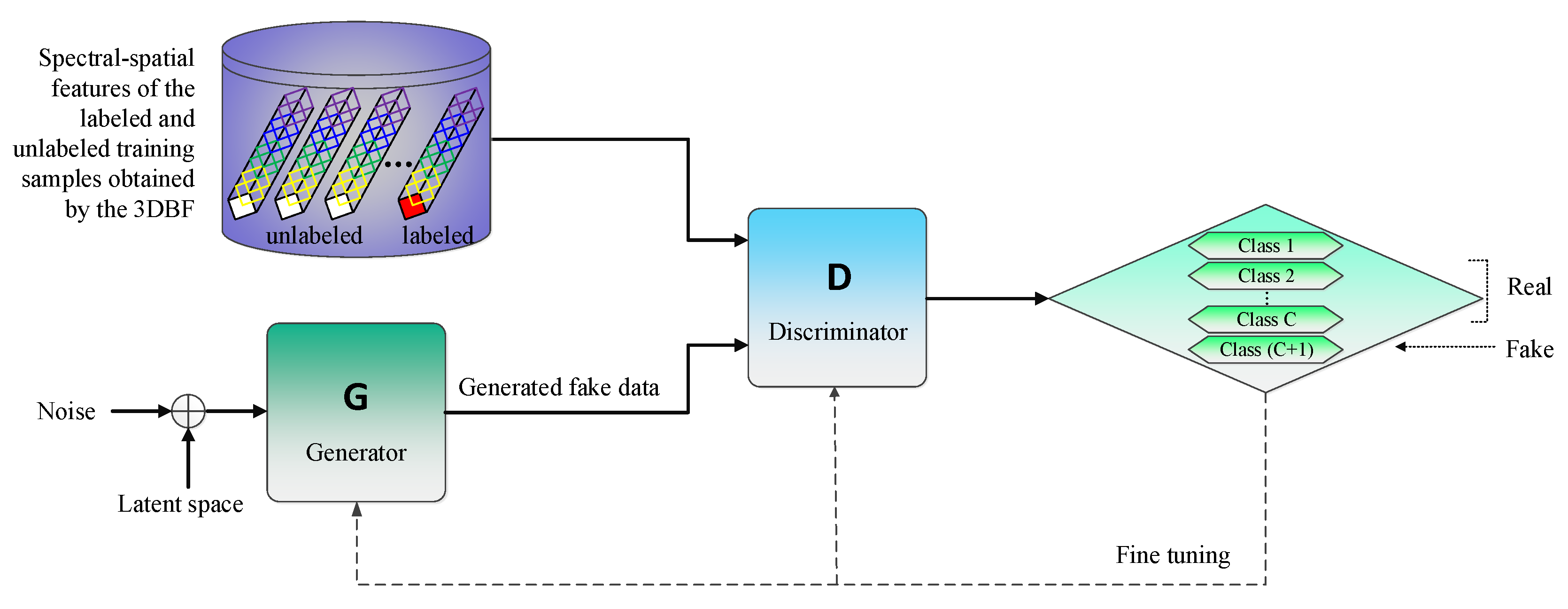
G matches the distribution of training data. Based on the above analysis, we show a visual illustration of the semi-supervised hyperspectral classification method by GANs in Figure 5. The network parameters of the generator G and the discriminator D in Figure 5 are trained by optimizing the loss function in Equation (17). The unlabeled data is taken as the true data s p data in Equation (19) to train both generator G and discriminator D. Moreover, the latent space of the generator G is chosen from the unlabeled data (To be exact, the latent space can also be chosen from the labeled data by ignoring the class labels), the noise follows the uniform distribution, and the output of the generator G is the fake data. By jointly minimizing the loss functions in Equation (17), the parameters of the generator G are updated to fool the discriminator D, and the fake examples are generated accordingly. The logistic regression classifier based on the soft-max function is adopted to perform the multi-class classification in the GANs. It is notable that the actual differences between the traditional GANs and the modified GANs used in this paper lie in threefold: (1) the objective functions are changed to make full use of both labeled and unlabeled samples; (2) the output layer of the discriminator is modified from binary classification to multi-class semi-supervised learning; (3) feature matching is adopted to improve the stability of the traditional GANs.

3. Experimental Section

In this section, we investigate the performance of the proposed method (abbreviated as 3DBF-GANs for simplicity) on three benchmark HSI datasets. A series of experiments are conducted to perform a comprehensive comparison with other state-of-the-art methods, including 2DBF [64], SVM [12], Laplacian SVM (LapSVM) [22,24] and CDL-MD-L [62]. 2DBF and 3DBF are feature extraction methods, SVM is a widely-used supervised classifier, while LapSVM, GANs and CDL-MD-L are classifiers based on semi-supervised learning. Moreover, the original spectral features are also considered as a baseline for comparison.

3.1. Dataset Description

In the experiments, three publicly available hyperspectral datasets (i.e., Indian Pines data, University of Pavia data and Salinas data) are employed as benchmark datasets. What follows are details of the three hyperspectral datasets.
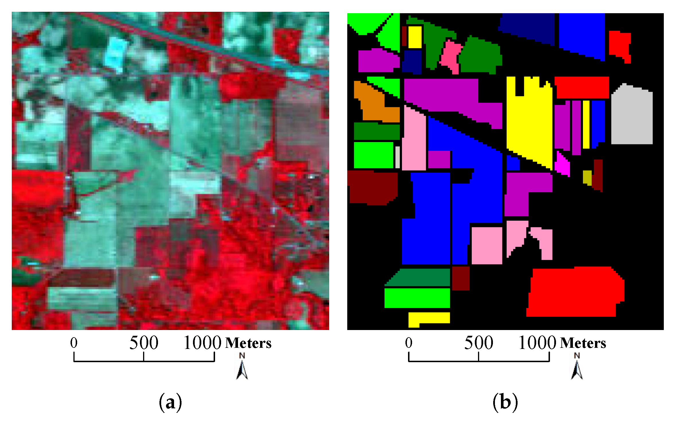
  • Indian Pines data: the first dataset was captured by the Airborne Visible/Infrared Imaging Spectrometer (AVIRIS) sensor over the agricultural Indian Pines test site in the Northwestern Indiana, USA, on 12 June 1992. The original image contains 224 spectral bands. After removing 4 bands full of zero and 20 bands affected by noise and water-vapor absorption, 200 bands are left for experiments. It consists of 145 × 145 pixels with a spatial resolution of 20 m per pixel, and the spectral coverage ranging from 0.4 to 2.5 μ m. Figure 6 depicts the color composite of the image as well as the ground truth map. There are 16 classes of interest and the number of samples in each class is displayed in Table 1, whose background color denotes different classes of land-covers. Since the number of samples is unbalanced and the spatial resolution is relatively low, it poses a big challenging to the classification task.
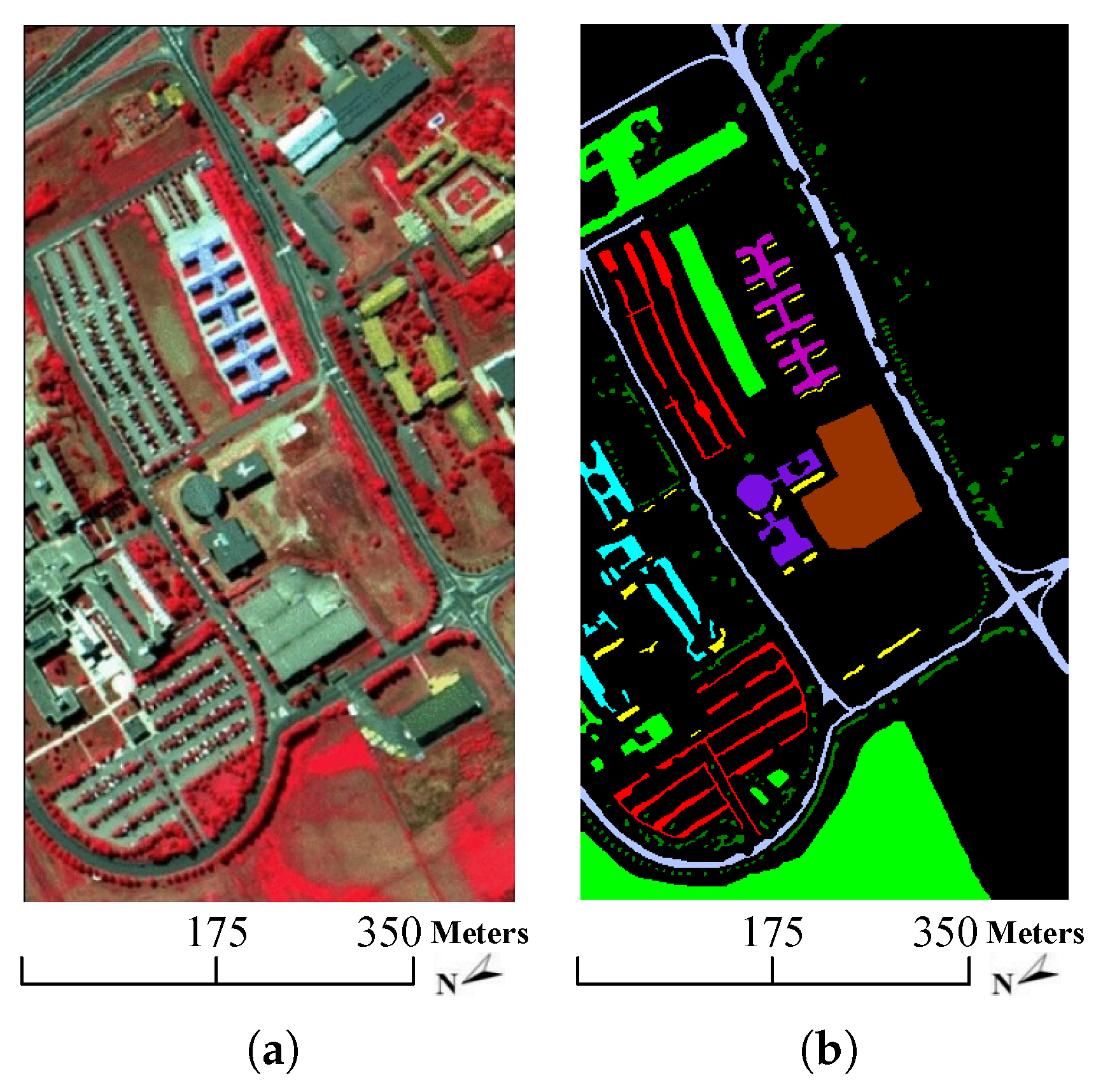
  • University of Pavia data: the second dataset was acquired by the Reflective Optics System Imaging Spectrometer (ROSIS) sensor over an urban area surrounding the University of Pavia, northern Italy, on 8 July 2002. The original data contains 115 spectral bands ranging from 0.43 to 0.86 μ m and the size of each band is 610 × 340 with a spatial resolution of 1.3 m per pixel. After removing 12 noisiest channels, 103 bands remained for experiments. The dataset contains 9 classes with various types of land-covers. The color composite image together with the ground truth data are shown in Figure 7. The detailed number of samples in each class is listed in Table 2, whose background color also corresponds to the color in Figure 7.
  • Salinas data: the third dataset was collected by the AVIRIS sensor over the Salinas Valley, Southern California, USA, on 8 October 1998. The original dataset contains 224 spectral bands covering from the visible to short-wave infrared light. After discording 20 water absorption bands, 204 bands are preserved for experiments. This dataset consists of 512 × 217 pixels with a spatial resolution of 3.7 m per pixel. The color composite of the image and the ground truth are plotted in Figure 8, which contains 16 classes of interest. The detailed number of classes in each class is shown in Table 3, whose background color represents different classes of land-covers.

3.2. Experimental Setup

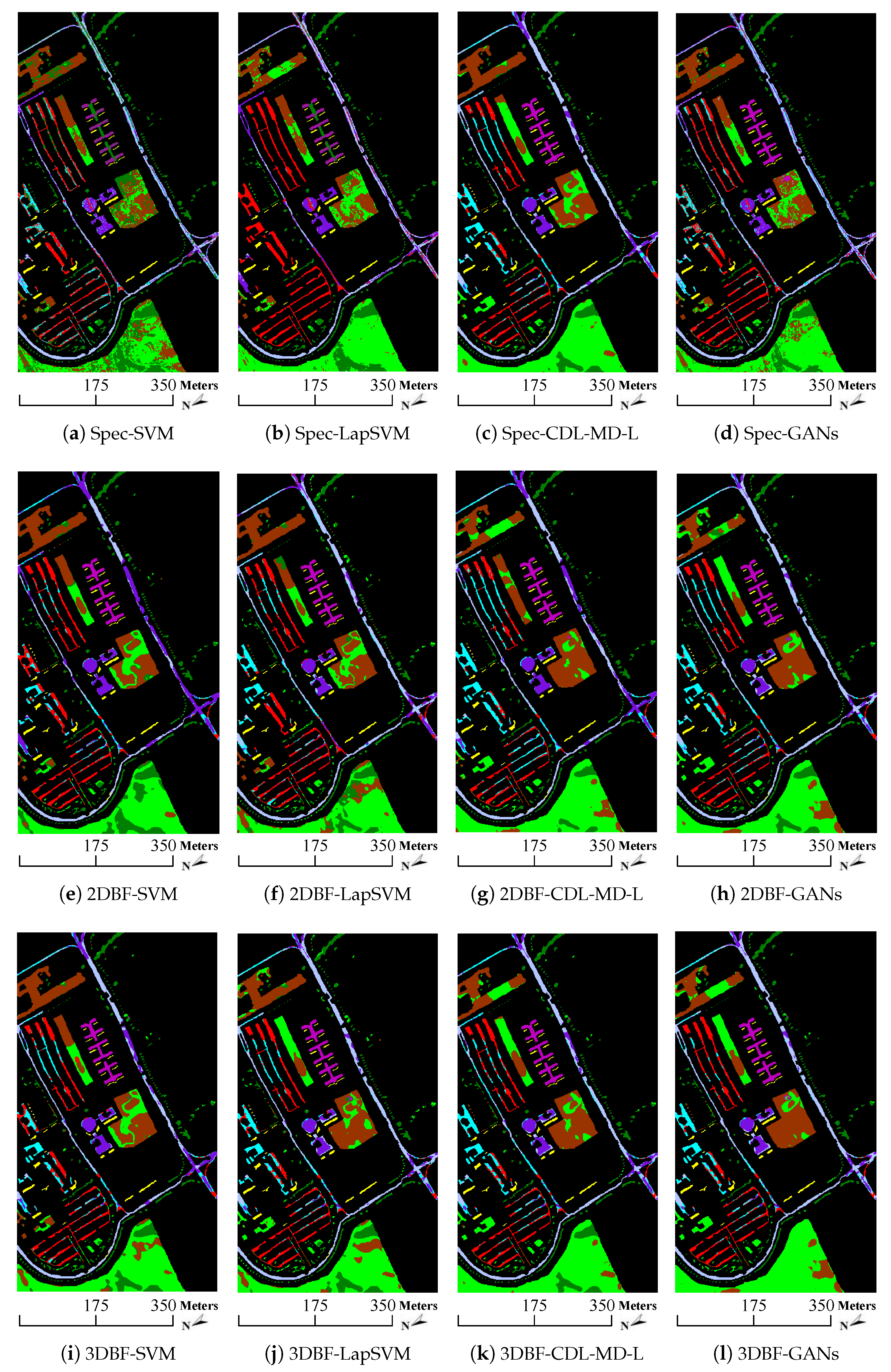
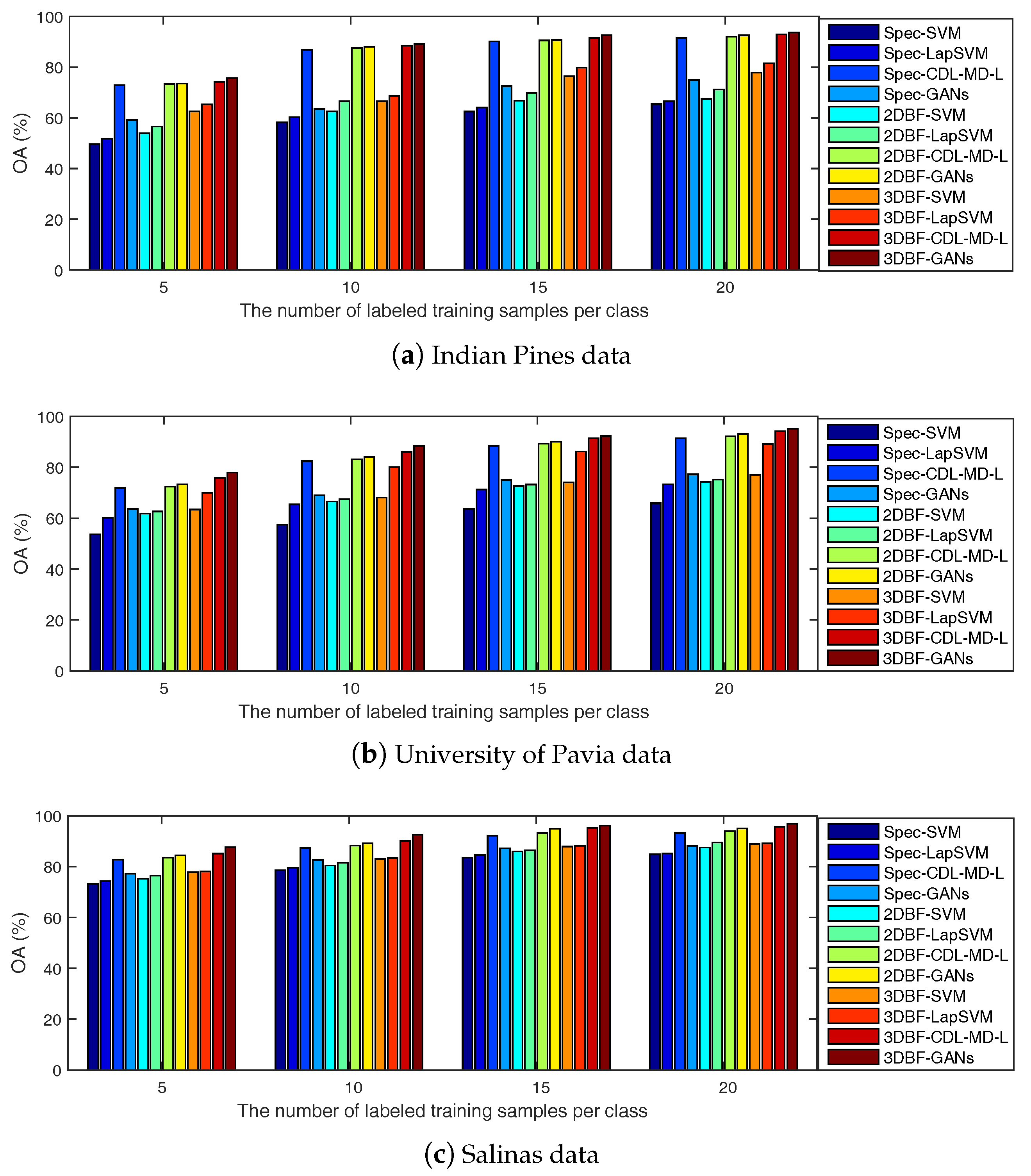
In order to evaluate the performance of the proposed 3DBF-GANs method, we compare it with some other algorithms, i.e., 2DBF, SVM, LapSVM, and CDL-MD-L. The original spectral features (abbreviated as “Spec”) are also considered in the experiments. Specifically, the “Spec”, 2DBF and 3DBF are feature extraction methods, while SVM, LapSVM and CDL-MD-L are supervised/semi-supervised classifiers. The LapSVM, which is a graph-based semi-supervised learning method, introduces an additional manifold regularizer on the geometry of both unlabeled and labeled data in terms of the Graph Laplacian. It has been applied to hyperspectral classification and the results have demonstrated the advantage of this graph-based method in semi-supervised classification of the HSI. As to the GANs, the standard framework is used, except for adding a softmax classifier in the output of the discriminator and adopting feature matching to improve the stability of the original GANs. By combining the feature extraction and classification methods in pairs, 12 methods (i.e., Spec-SVM, Spec-LapSVM, Spec-GANs, Spec-CDL-MD-L, 2DBF-SVM, 2DBF-LapSVM, 2DBF-CDL-MD-L, 2DBF-GANs, 3DBF-SVM, 3DBF-LapSVM, 3DBF-CDL-MD-L and 3DBF-GANs) are obtained for comparison. Since the spectral-spatial information is used in the original CDL-MD-L, Spec-CDL-MD-L and 3DBF-CDL-MD-L denote the input of the CDL-MD-L is the original HSI and the dataset given by 3DBF, respectively.
In the experiments, a training/test sample is a single pixel, whose size is 1 × b . Each pixel can be taken as the feature of a certain class and classified by the discriminator of the GANs or other classifiers. Each pixel corresponds to a unique label. The whole cube contains many pixels and therefore, has lots of labels. All the HSI datasets are normalized between zero and one at the beginning of the experiments. All the experiments are implemented on the normalized hyperspectral datasets, whose available data is randomly divided into two parts, i.e., about 60% for training and the rest for testing. In all the datasets, very limited labeled samples, i.e., 5 samples per class, are randomly selected from the training samples as labeled samples, and the remaining ones are used as unlabeled samples. The experiments are repeated ten times using random selection of training and test sets, and the average accuracies are reported. To assess the experimental results quantitatively, we compare the aforementioned methods by three popular indexes, i.e., overall accuracy (OA), average accuracy (AA) and kappa coefficient ( κ ). Moreover, the F-Measure of various methods is also compared.
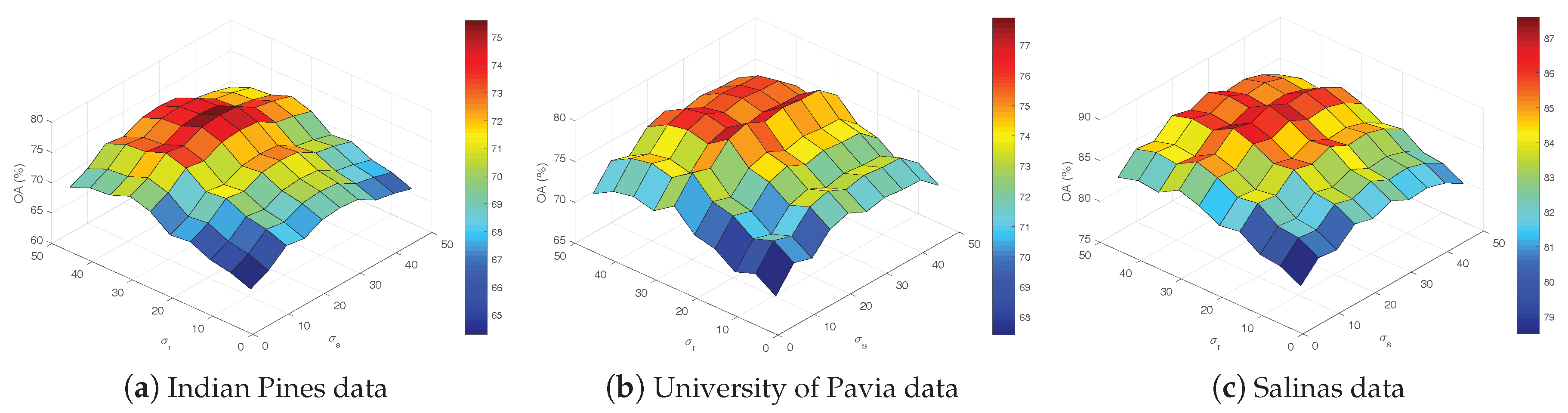
For the parameter settings, since the number of labeled samples is limited, leave one out cross validation is adopted in this paper. The range of the filtering size σ s and blur degree σ r in the 2DBF are selected in the range of [ 1 , 2 , , 9 ] and [ 0.1 , 0.2 , , 0.5 ] , respectively, whereas both σ s and σ r in the 3DBF are chosen from [ 5 , 10 , , 50 ] . In the SVM and LapSVM, radial basis function (RBF) kernels are adopted. The RBF parameter γ is obtained from the range [ 2 2 , 2 1 , , 2 10 ] and the penalty term is set to 60. 4 spectral neighbors are adopted to calculate the Laplacian graph in the LapSVM. Three layers are used in the CDL-MD-L, whose window size and the number of hidden units are set to the same as [62]. The generator in the GANs has two hidden layers, and the number of units is set to 500 and 300, respectively. In the discriminator, three hidden layers are adopted, and the number of units is set to 300 , 200 
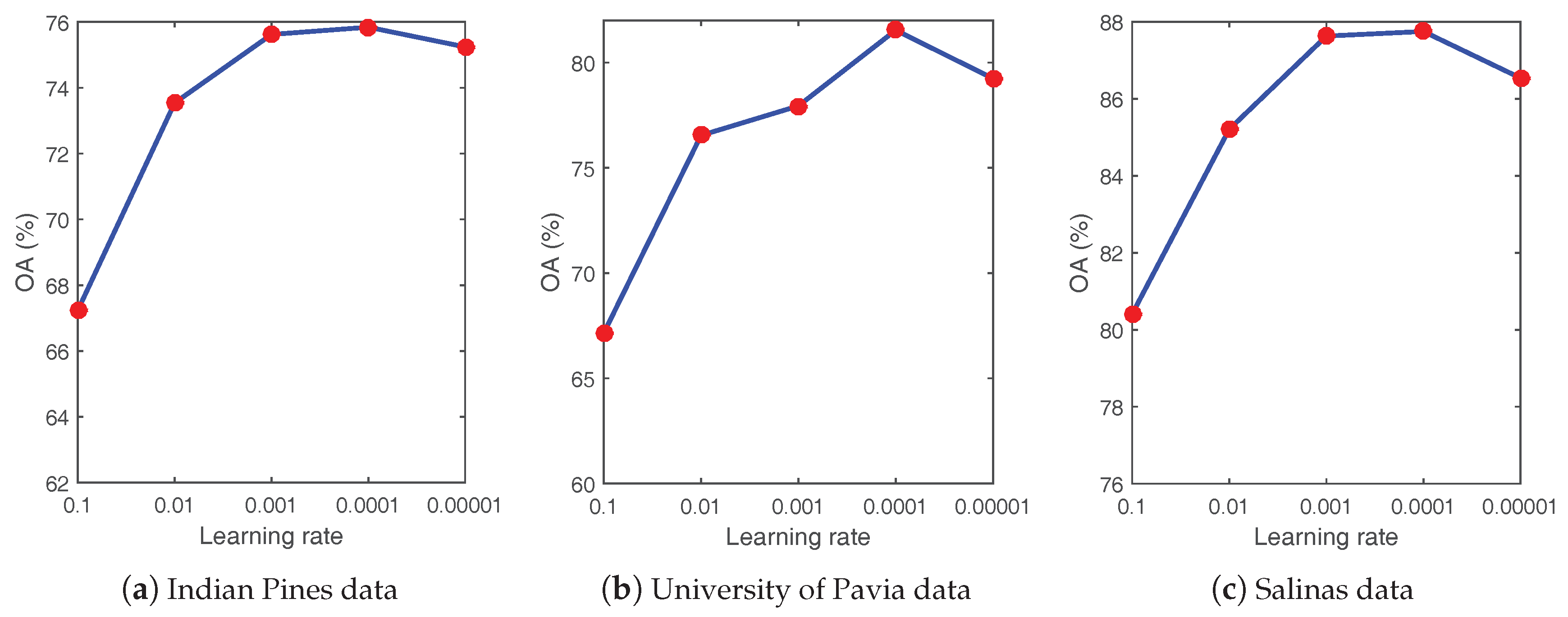
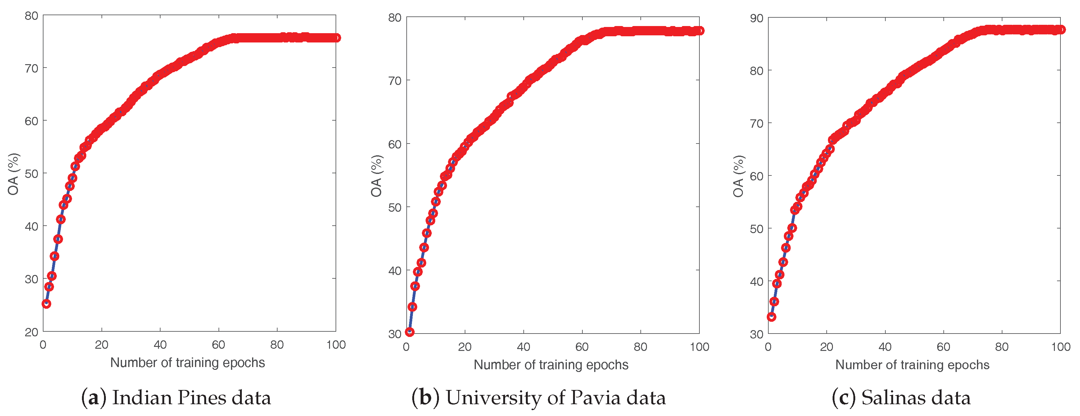
and 150, respectively. Gaussian noise is added to the output of each layer of the discriminator. Moreover, the learning rate and training epoch are set to 0.001 and 100, respectively.

3.3. Experimental Results

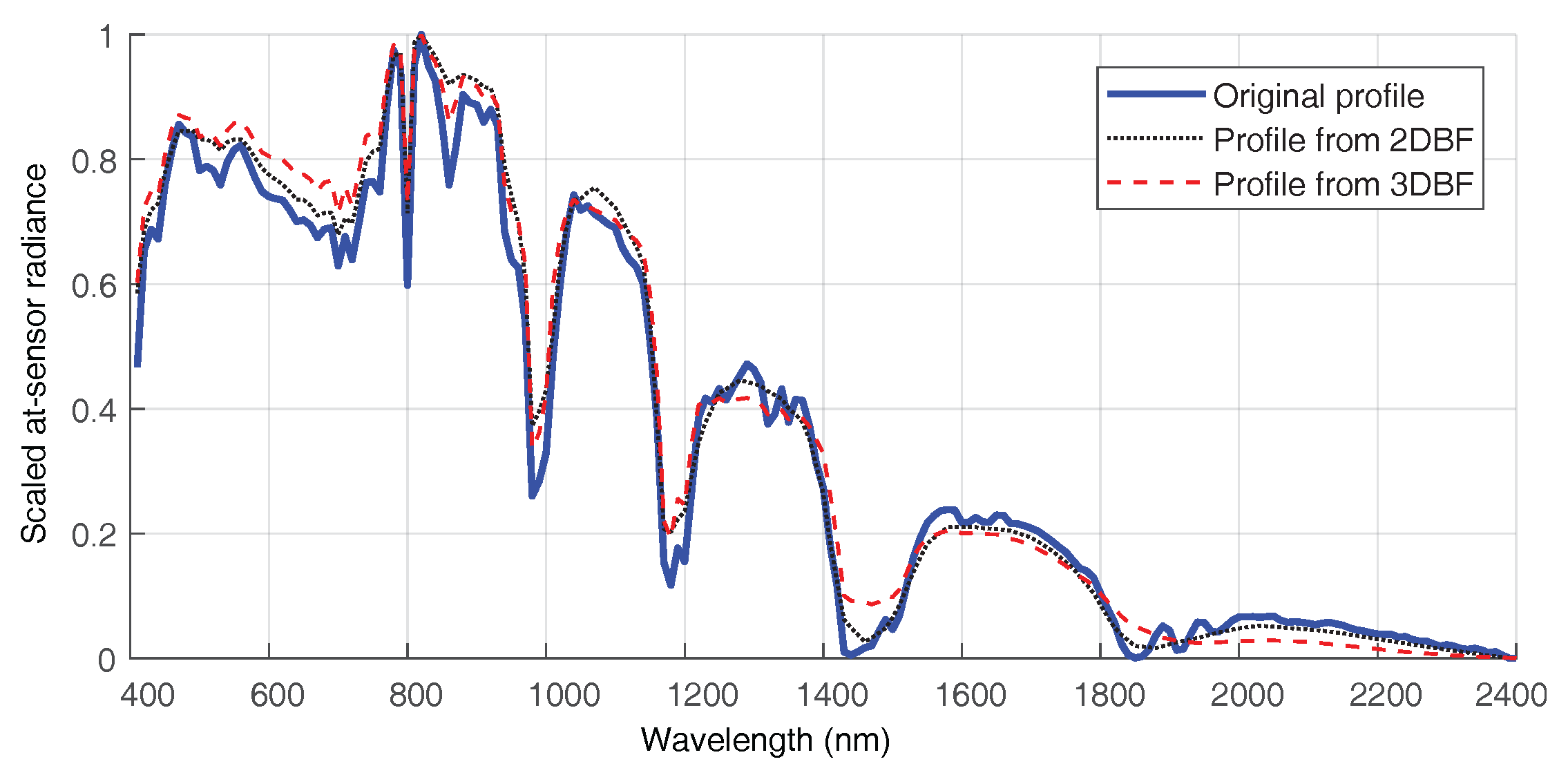
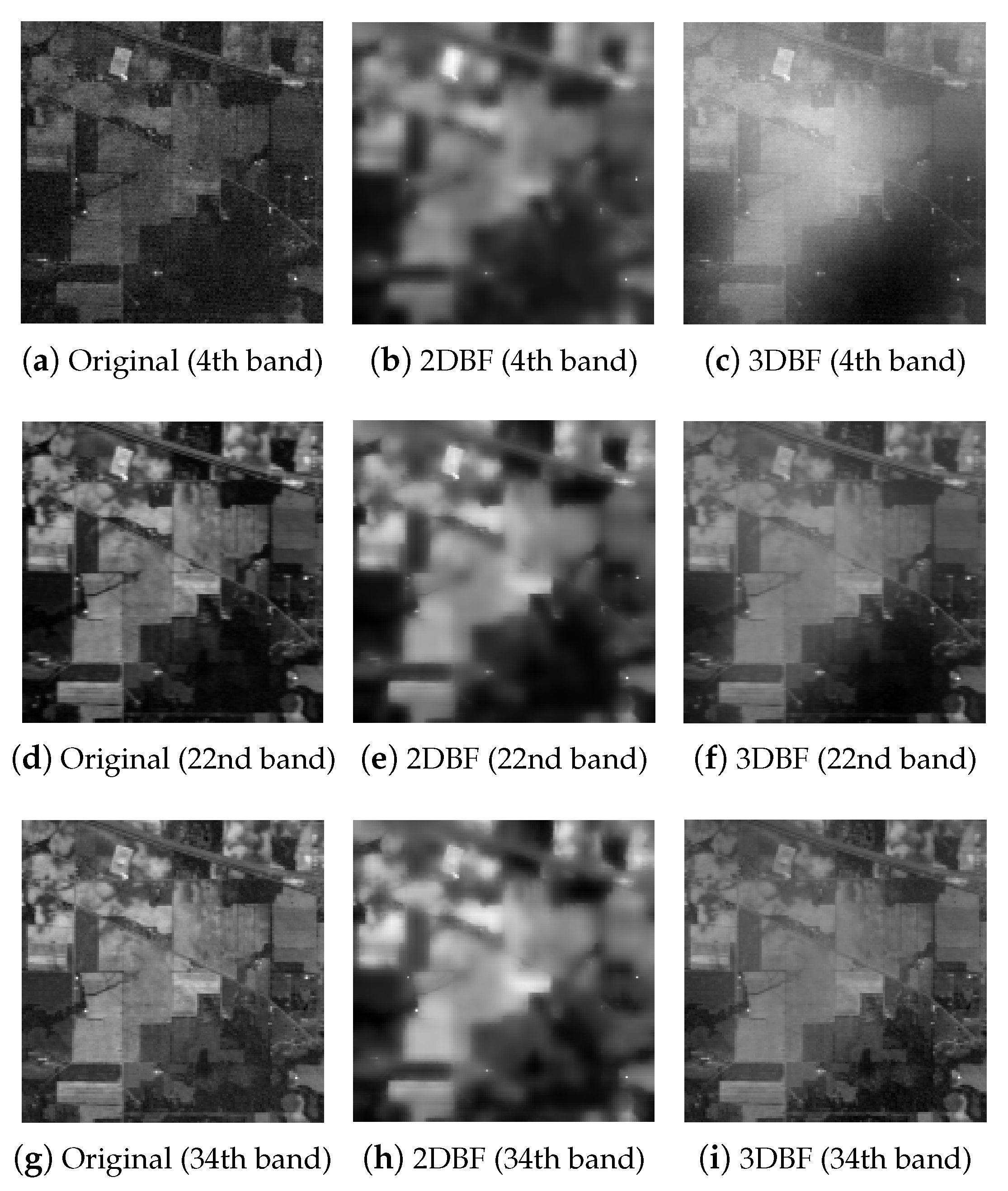
To demonstrate the effectiveness of the 3DBF for spectral-spatial feature extraction, we compare the spectral profiles of the pixel (18,6) from the original Indian Pines data, and the features obtained by the 2DBF and the 3DBF in Figure 9. Moreover, the spatial scenes of the 4th, 22nd, 34th bands are compared in Figure 10. As can be seen, the profiles of 3DBF preserve the trend of the original data while provide smoother features in both spectral and spatial domains.
The qualitative evaluations of various methods are shown in Table 4, Table 5 and Table 6, and the classification maps are also visually compared in
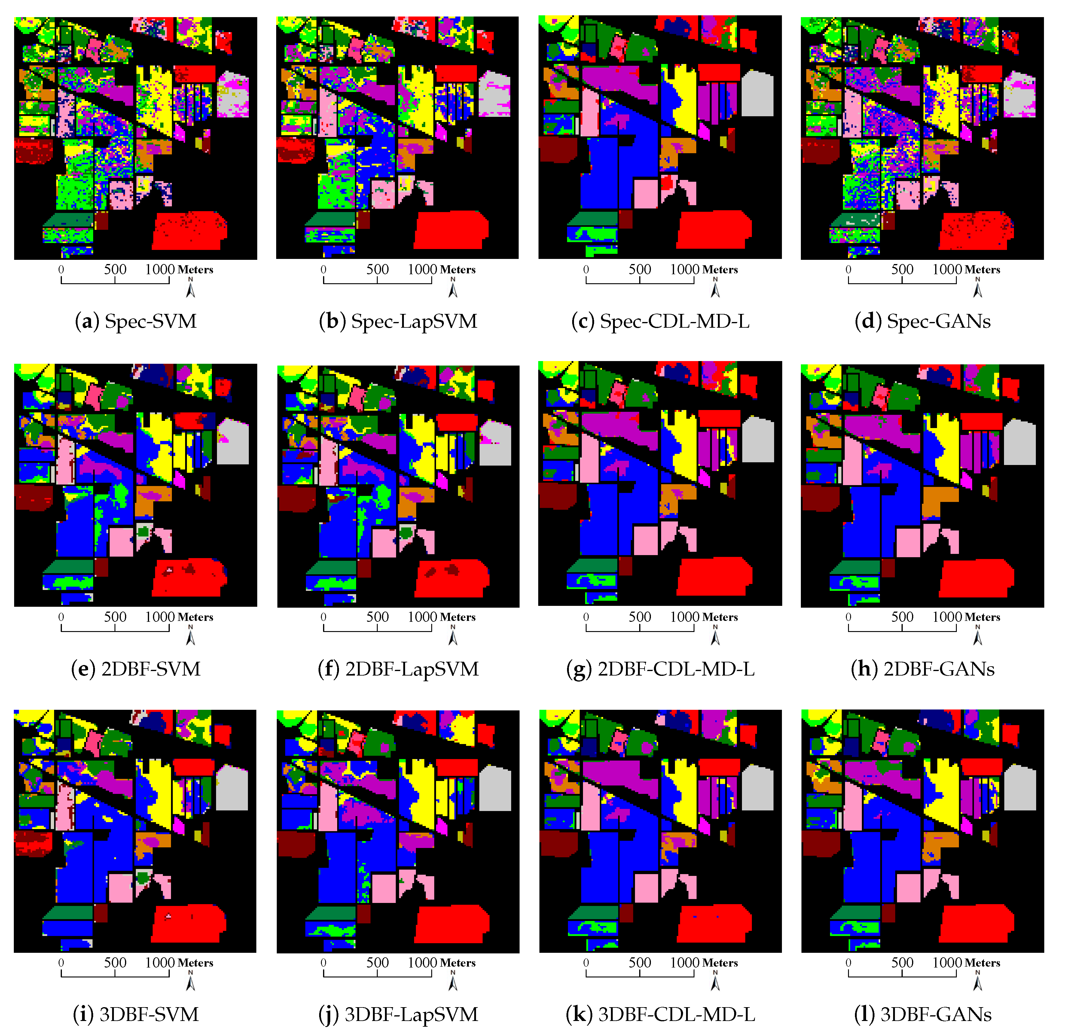
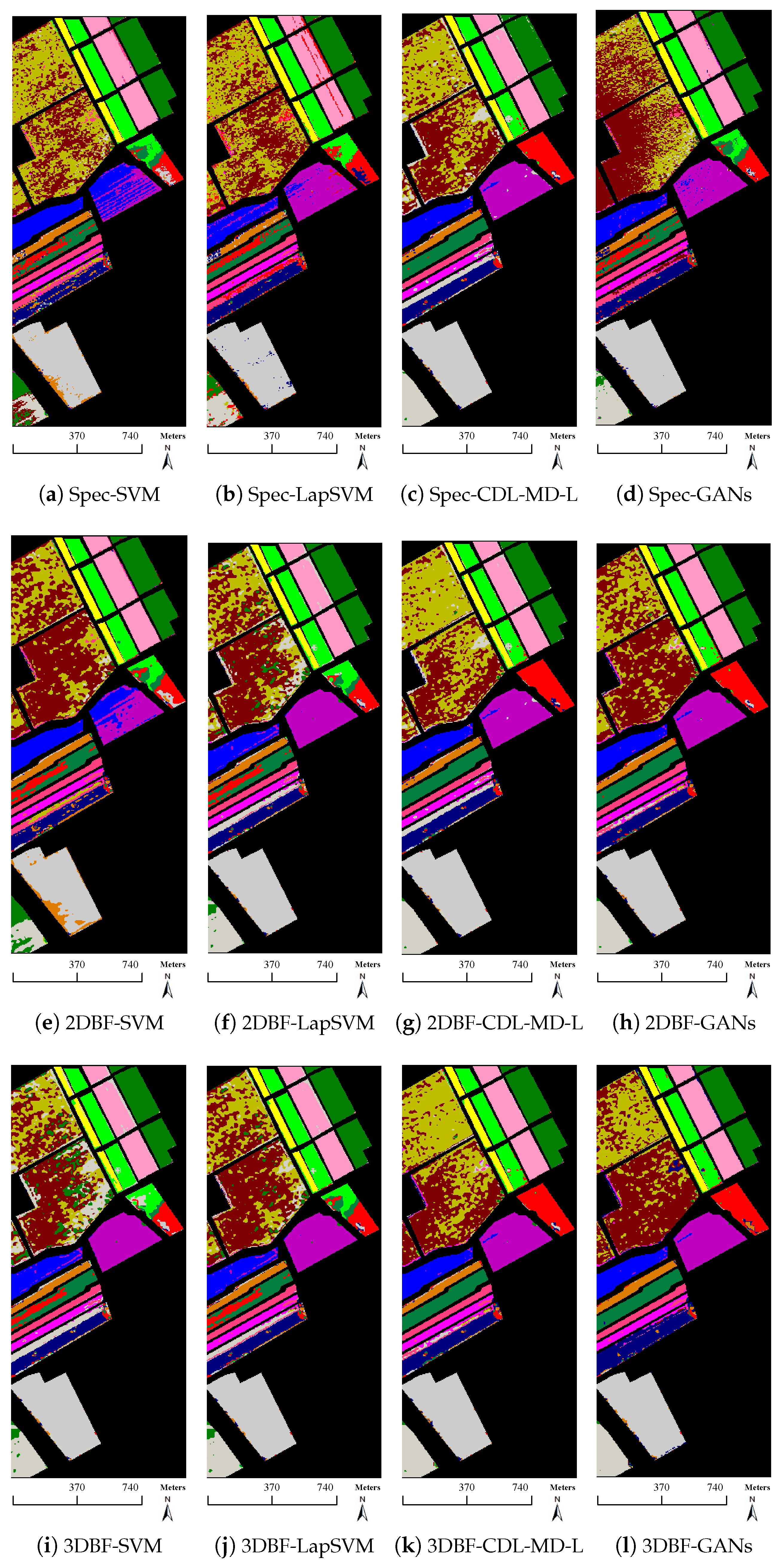
 Figure 11, Figure 12 and Figure 13. Based on the above-mentioned experimental results, a few observations and discussions can be highlighted. It can be first seen that, the methods (i.e., Spec-SVM, 2DBF-SVM, and 3DBF-SVM) using only the limited labeled training samples provide worse classification performance than the semi-supervised methods that take the unlabeled training samples into consideration. This stresses yet again the importance of unlabeled samples for HSI classification. For instance, it is observed from Table 4 that the SVM leads to lower classification accuracies than other classifiers (i.e., LapSVM, CDL-MD-L and GANs). Taking the same original “Spec” features as inputs, the OA of SVM is 2.15%, 23.28% and 9.49% lower than those of the LapSVM, CDL-MD-L and GANs, respectively. Similar properties can also be found in Table 5 and Table 6. The above-mentioned phenomena demonstrate the effectiveness of utilizing the abundant unlabeled samples for the HSI data.
Second, the “Spec”-based features provide higher classification errors than the 2DBF/3DBF-based features. As shown in Table 5, the OA, AA, κ and F-Measure of Spec-SVM are lower than those of the 2DBF-SVM and 3DBF-SVM. Similarly, the OA, AA, κ and F-Measure of Spec-LapSVM/ CDL-MD-L/GANs are also lower than 2DBF-LapSVM/CDL-MD-L/GANs and 3DBF-LapSVM/ CDL-MD-L/GANs. It is also clearly visible that more scattered noise is generated in Figure 12a than in Figure 12e,i. This is due to the fact that the “Spec” features based only on spectral characteristics, while 2DBF and 3DBF methods can effectively incorporate the spatial information. Since the CDL-MD-L can make use of both spectral and spatial information in the classification process, the classification accuracies of Spec-CDL-MD-L are much higher than those of the Spec-SVM, Spec-LapSVM and Spec-GANs. As shown in Table 5, the OA of Spec-CDL-MD-L is at least 8% higher than other classifiers. Moreover, with the same classifiers, the 3DBF performs much better than 2DBF. For instance, the OA of 3DBF-GANs in Table 5 is about 4% higher than that of the 2DBF-GANs. The reason for good results of 3DBF is that it exploits the spectral-spatial features by obeying the 3D nature of the HSI cube.
Finally, as to different classifiers, the GANs with 2DBF or 3DBF features provides better or comparable classification results as compared with SVM, LapSVM and CDL-MD-L. It is observed from Table 4 that the OA of 2DBF-GANs is 19.65%, 17.02% and 0.25% higher than those of the 2DBF-SVM, 2DBF-LapSVM and 2DBF-CDL-MD-L, respectively, the OA of 3DBF-GANs is also much higher than 3DBF-SVM and 3DBF-LapSVM, and slightly higher than 3DBF-CDL-MD-L. Classification results of the University of Pavia data (see Table 5) and the Salinas data (see Table 6) also yield similar properties. Specifically, it is noteworthy that the “meadows” (i.e., class 2) and “bare soil” (i.e., class 6) in the University of Pavia are difficult to be separated, and the classification accuracies of those two classes obtained by the 3DBF-GANs outperform other methods (see Table 5). Moreover, the GANs with the original spectral features are much inferior to the CDL-MD-L. As shown in Table 4, the OA of Spec-GANs is 13.79% less than that of the Spec-CDL-MD-L. In Table 5 (or Table 6), the OA of Spec-GANs is also 8.17% (or 5.55%) lower than the Spec-CDL-MD-L. The main reason why Spec-GANs obtains poor results is the ignorance of spatial information. In a nutshell, the afore-mentioned analysis validates the effectiveness of the proposed 3DBF-GANs method in semi-supervised hyperspectral classification.

4. Discussions

4.1. Statistical Significance Analysis of the Results

The statistical significance of the classification differences between various methods is assessed by the McNemar’s test, which is based upon the standardized normal test statistic
Z = f 12 f 21 f 12 + f 21
where f i j refers to the number of samples classified correctly by the classifier i but incorrectly by classifier j and Z indicates the pairwise statistical significance of the classification difference between the ith and jth classifiers. In case the test statistic | Z | > 1.96 , the difference of classification accuracies between the ith and jth classifiers is regarded as statistical significant at the 5% level of significance. For comparison purpose, the results of the McNemar’s test on the 3DBF-GANs and other methods are listed in Table 7, which shows that the proposed 3DBF-GANs is superior ( Z > 1.96 ) to Spec-SVM, Spec-LapSVM, Spec-GANs, Spec-CDL-MD-L, 2DBF-SVM, 2DBF-LapSVM, 2DBF-CDL-MD-L, 2DBF-GANs, 3DBF-SVM, 3DBF-LapSVM, or comparable ( | Z | < 1.96 in the Indian Pines data) with 3DBF-CDL-MD-L. According to the McNemar’s test, both the 3DBF and GANs are helpful for improving the classification performance since the test statistic is statistical significant, which further confirms the effectiveness of the proposed method.

4.2. Sensitivity Analysis of the Parameters

There are four important parameters in the proposed 3DBF-GANs method: the filtering size σ s , the blur degree σ r , the training epoch and the learning rate. The influence of these parameters on the classification performance (e.g., OA) is analyzed in Figure 14 and Figure 15. In Figure 14, the effect of σ s and σ r is plotted with the training epoch is fixed to 100. It can be seen from Figure 14 that, if the filtering size σ s and the blur degree σ r are too small or too large, the OA of 3DBF-GANs is not satisfactory. This is due to the fact that very little spatial information is considered in case σ s and σ r are too small, while too large σ s and σ r will cause oversmooth. Furthermore, the influence of the training epoch is depicted in Figure 15, from which one can observe that, the OA rapidly increases at first, then slowly increases and finally trends to a certain stable value with the increasing of training epoch. The influence of the learning rate is shown in Figure 16, from which one can find that the OA with a large learning rate (e.g., 0.1) is much lower than that with a smaller learning rate. The reason is that too large learning rate can cause the loss function to fluctuate around the minimum, or even worse, to diverge. Note that too small (e.g., 0.00001) will lead to slow convergence, it is better to set the learning rate to 0.001 or 0.0001. In analogy to the other comparison methods, the appropriate parameters are of importance to the classification performance our proposed 3DBF-GANs method. It is highlighted from the above analysis that we are able to gain satisfying classification results for different hyperspectral datasets with the provided parameter settings.
Moreover, the impact of the number of labeled training samples is also evaluated in this section. We randomly choose 5, 10, 15 and 20 samples from each class as the labeled training samples and the OA of various methods is plotted in Figure 17, which shows that the classification accuracy increases as the number of labeled training samples goes up and the 3DBF-GANs method is superior to other methods when the same number of labeled training samples is chosen. Although the performance of different methods changes as the number of training samples changes, the 3DBF-GANs provides higher classification accuracies than other methods. In addition, it should be pointed out here that the number of synthetic examples generated by the 3DBF-GANs method equals to the total number of training samples (including labeled samples and unlabeled samples), and therefore, is not varied with the number of labeled samples.

5. Conclusions

In this paper, we have proposed a semi-supervised learning method based on 3DBF and GANs for hyperspectral classification. The proposed 3DBF-GANs method relies on two aspects. The first is the extraction of spectral-spatial features by the 3DBF. The main advantage of the 3DBF is that it is able to smooth the hyperspectral cube while preserving the edges by naturally treating the HSI as a volumetric dataset. The second one is the semi-supervised classification by the GANs. The GANs can make full use of both the limited labeled samples and the abundance of unlabeled samples for significant semi-supervised learning. Compared to the shallow learning and non-adversarial networks, the GANs are one of the effective deep learning methods which can take advantage of the discriminative models to train the generative network in an adversarial fashion. The proposed method has been tested on AVIRIS and ROSIS datasets with very limited labeled samples, and the comparison with other state-of-the-art methods (i.e., 2DBF, SVM, LapSVM, and CDL-MD-L) has confirmed the effectiveness of the proposed method. Quantitatively, the OA of 3DBF-GANs improves about 1% to 25% compared to other state-of-the-art methods. Note that the GANs have a complex structure, a future research topic is to investigate how to determine the network parameters in a more effective and automatic way. Introducing the graph-based semi-supervised learning method [26] from other areas to hyperspectral classification is also a probable future research direction.

Acknowledgments

This work was supported by the National Natural Science Foundation of China under Grant 41501368, and the Fundamental Research Funds for the Central Universities under Grant 16lgpy04. The authors would like to thank D. Landgrebe from Purdue University for providing the AVIRIS image of Indian Pines and the Gamba from University of Pavia for providing the ROSIS data set. Last but not least, we would like to take this opportunity to thank the Editors and the Anonymous Reviewers for their detailed comments and suggestions, which greatly helped us to improve the clarity and presentation of our manuscript.

Author Contributions

All coauthors made significant contributions to the manuscript. Zhi He and Han Liu designed the research framework, analyzed the results and wrote the manuscript. Jie Hu and Yiwen Wang assisted in the prepared work and validation work. Moreover, all coauthors contributed to the editing and review of the manuscript.

Conflicts of Interest

The authors declare no conflict of interest.

References

  1. Sun, W.; Jiang, M.; Li, W.; Liu, Y. A symmetric sparse representation based band selection method for hyperspectral imagery classification. Remote Sens. 2016, 8, 238. [Google Scholar] [CrossRef]
  2. Sun, W.; Zhang, D.; Xu, Y.; Tian, L.; Yang, G.; Li, W. A probabilistic weighted archetypal analysis method with earth mover’s distance for endmember extraction from hyperspectral imagery. Remote Sens. 2017, 9, 841. [Google Scholar] [CrossRef]
  3. Pan, L.; Li, H.C.; Deng, Y.J.; Zhang, F.; Chen, X.D.; Du, Q. Hyperspectral dimensionality reduction by tensor sparse and low-rank graph-based discriminant analysis. Remote Sens. 2017, 9, 452. [Google Scholar] [CrossRef]
  4. Feng, F.; Li, W.; Du, Q.; Zhang, B. Dimensionality reduction of hyperspectral image with graph-based discriminant analysis considering spectral similarity. Remote Sens. 2017, 9, 323. [Google Scholar] [CrossRef]
  5. Gao, L.; Zhao, B.; Jia, X.; Liao, W.; Zhang, B. Optimized kernel minimum noise fraction transformation for hyperspectral image classification. Remote Sens. 2017, 9, 548. [Google Scholar] [CrossRef]
  6. Sun, B.; Kang, X.; Li, S.; Benediktsson, J.A. Random-walker-based collaborative learning for hyperspectral image classification. IEEE Trans. Geosci. Remote Sens. 2017, 55, 212–222. [Google Scholar] [CrossRef]
  7. Yang, L.; Wang, M.; Yang, S.; Zhang, R.; Zhang, P. Sparse spatio-spectral LapSVM with semisupervised kernel propagation for hyperspectral image classification. IEEE J. Sel. Top. Appl. Earth Obs. Remote Sens. 2017, 10, 2046–2054. [Google Scholar] [CrossRef]
  8. Zhong, Y.; Ma, A.; Zhang, L. An adaptive memetic Fuzzy clustering algorithm with spatial information for remote sensing imagery. IEEE J. Sel. Top. Appl. Earth Obs. Remote Sens. 2014, 7, 1235–1248. [Google Scholar] [CrossRef]
  9. Niazmardi, S.; Homayouni, S.; Safari, A. An improved FCM algorithm based on the SVDD for unsupervised hyperspectral data classification. IEEE J. Sel. Top. Appl. Earth Obs. Remote Sens. 2013, 6, 831–839. [Google Scholar] [CrossRef]
  10. Zhong, Y.; Zhang, L.; Huang, B.; Li, P. An unsupervised artificial immune classifier for multi/hyperspectral remote sensing imagery. IEEE Trans. Geosci. Remote Sens. 2006, 44, 420–431. [Google Scholar] [CrossRef]
  11. Zhu, W.; Chayes, V.; Tiard, A.; Sanchez, S.; Dahlberg, D.; Bertozzi, A.L.; Osher, S.; Zosso, D.; Kuang, D. Unsupervised classification in hyperspectral imagery with nonlocal total variation and primal-dual hybrid gradient algorithm. IEEE Trans. Geosci. Remote Sens. 2017, 55, 2786–2798. [Google Scholar] [CrossRef]
  12. Vapnik, V. The Nature of Statistical Learning Theory; Springer Science & Business Media: New York, NY, USA, 2013. [Google Scholar]
  13. Kuo, B.C.; Ho, H.H.; Li, C.H.; Hung, C.C.; Taur, J.S. A kernel-based feature selection method for SVM with RBF kernel for hyperspectral image classification. IEEE J. Sel. Top. Appl. Earth Obs. Remote Sens. 2014, 7, 317–326. [Google Scholar]
  14. Adep, R.N.; Shetty, A.; Ramesh, H. EXhype: A tool for mineral classification using hyperspectral data. ISPRS J. Photogramm. Remote Sens. 2017, 124, 106–118. [Google Scholar] [CrossRef]
  15. Chen, Y.; Nasrabadi, N.M.; Tran, T.D. Hyperspectral image classification via kernel sparse representation. IEEE Trans. Geosci. Remote Sens. 2013, 51, 217–231. [Google Scholar] [CrossRef]
  16. Zhang, Y.; Du, B.; Zhang, L.; Liu, T. Joint sparse representation and multitask learning for hyperspectral target detection. IEEE Trans. Geosci. Remote Sens. 2017, 55, 894–906. [Google Scholar] [CrossRef]
  17. Li, J.; Bioucas-Dias, J.M.; Plaza, A. Semisupervised hyperspectral image classification using soft sparse multinomial logistic regression. IEEE Geosci. Remote. Sens. Lett. 2013, 10, 318–322. [Google Scholar]
  18. Chapel, L.; Burger, T.; Courty, N.; Lefevre, S. PerTurbo manifold learning algorithm for weakly labeled hyperspectral image classification. IEEE J. Sel. Top. Appl. Earth Obs. Remote Sens. 2014, 7, 1070–1078. [Google Scholar] [CrossRef]
  19. Joachims, T. Transductive inference for text classification using support vector machines. In Proceedings of the Sixteenth International Conference on Machine Learning, San Francisco, CA, USA, 27–30 June 1999; pp. 200–209. [Google Scholar]
  20. Maulik, U.; Chakraborty, D. Learning with transductive SVM for semisupervised pixel classification of remote sensing imagery. ISPRS J. Photogramm. Remote Sens. 2013, 77, 66–78. [Google Scholar] [CrossRef]
  21. Wang, L.; Hao, S.; Wang, Q.; Wang, Y. Semi-supervised classification for hyperspectral imagery based on spatial-spectral label propagation. ISPRS J. Photogramm. Remote Sens. 2014, 97, 123–137. [Google Scholar] [CrossRef]
  22. Belkin, M.; Niyogi, P.; Sindhwani, V. Manifold regularization: A geometric framework for learning from labeled and unlabeled examples. J. Mach. Learn. Res. 2006, 7, 2399–2434. [Google Scholar]
  23. Camps-Valls, G.; Marsheva, T.V.B.; Zhou, D. Semi-supervised graph-based hyperspectral image classification. IEEE Trans. Geosci. Remote Sens. 2007, 45, 3044–3054. [Google Scholar] [CrossRef]
  24. Melacci, S.; Belkin, M. Laplacian support vector machines trained in the primal. J. Mach. Learn. Res. 2011, 12, 1149–1184. [Google Scholar]
  25. De Morsier, F.; Borgeaud, M.; Gass, V.; Thiran, J.P.; Tuia, D. Kernel low-rank and sparse graph for unsupervised and semi-supervised classification of hyperspectral images. IEEE Trans. Geosci. Remote Sens. 2016, 54, 3410–3420. [Google Scholar] [CrossRef]
  26. Yamaguchi, Y.; Faloutsos, C.; Kitagawa, H. Camlp: Confidence-aware modulated label propagation. In Proceedings of the 2016 SIAM International Conference on Data Mining, SIAM, Miami, FlL, USA, 5–7 May 2016; pp. 513–521. [Google Scholar]
  27. Dopido, I.; Li, J.; Marpu, P.R.; Plaza, A.; Dias, J.M.B.; Benediktsson, J.A. Semisupervised self-learning for hyperspectral image classification. IEEE Trans. Geosci. Remote Sens. 2013, 51, 4032–4044. [Google Scholar] [CrossRef]
  28. Aydemir, M.S.; Bilgin, G. Semisupervised hyperspectral image classification using small sample sizes. IEEE Geosci. Remote. Sens. Lett. 2017, 14, 621–625. [Google Scholar] [CrossRef]
  29. Zhang, X.; Song, Q.; Liu, R.; Wang, W.; Jiao, L. Modified co-training with spectral and spatial views for semisupervised hyperspectral image classification. IEEE J. Sel. Top. Appl. Earth Obs. Remote Sens. 2014, 7, 2044–2055. [Google Scholar] [CrossRef]
  30. Romaszewski, M.; Głomb, P.; Cholewa, M. Semi-supervised hyperspectral classification from a small number of training samples using a co-training approach. ISPRS J. Photogramm. Remote Sens. 2016, 121, 60–76. [Google Scholar] [CrossRef]
  31. Fauvel, M.; Tarabalka, Y.; Benediktsson, J.A.; Chanussot, J.; Tilton, J.C. Advances in spectral-spatial classification of hyperspectral images. Proc. IEEE 2013, 101, 652–675. [Google Scholar] [CrossRef]
  32. Cavallaro, G.; Mura, M.D.; Benediktsson, J.A.; Bruzzone, L. Extended self-dual attribute profiles for the classification of hyperspectral images. IEEE Geosci. Remote Sens. Lett. 2015, 12, 1690–1694. [Google Scholar] [CrossRef]
  33. Bao, R.; Xia, J.; Mura, M.D.; Du, P.; Chanussot, J.; Ren, J. Combining morphological attribute profiles via an ensemble method for hyperspectral image classification. IEEE Geosci. Remote Sens. Lett. 2016, 13, 359–363. [Google Scholar] [CrossRef]
  34. Jia, S.; Shen, L.; Li, Q. Gabor feature-based collaborative representation for hyperspectral imagery classification. IEEE Trans. Geosci. Remote Sens. 2015, 53, 1118–1129. [Google Scholar]
  35. He, L.; Li, J.; Plaza, A.; Li, Y. Discriminative low-rank Gabor filtering for spectral–spatial hyperspectral image classification. IEEE Trans. Geosci. Remote Sens. 2017, 55, 1381–1395. [Google Scholar] [CrossRef]
  36. Kang, X.; Li, S.; Benediktsson, J.A. Spectral-spatial hyperspectral image classification with edge-preserving filtering. IEEE Trans. Geosci. Remote Sens. 2014, 52, 2666–2677. [Google Scholar] [CrossRef]
  37. Demir, B.; Erturk, S. Empirical mode decomposition of hyperspectral images for support vector machine classification. IEEE Trans. Geosci. Remote Sens. 2010, 48, 4071–4084. [Google Scholar] [CrossRef]
  38. He, Z.; Wang, Q.; Shen, Y.; Jin, J.; Wang, Y. Multivariate gray model-based BEMD for hyperspectral image classification. IEEE Trans. Instrum. Meas. 2013, 62, 889–904. [Google Scholar] [CrossRef]
  39. Zabalza, J.; Ren, J.; Zheng, J.; Han, J.; Zhao, H.; Li, S.; Marshall, S. Novel two-dimensional singular spectrum analysis for effective feature extraction and data classification in hyperspectral imaging. IEEE Trans. Geosci. Remote Sens. 2015, 53, 4418–4433. [Google Scholar] [CrossRef]
  40. Tarabalka, Y.; Chanussot, J.; Benediktsson, J. Segmentation and classification of hyperspectral images using watershed transformation. Pattern Recognit. 2010, 43, 2367–2379. [Google Scholar] [CrossRef]
  41. Li, J.; Zhang, H.; Zhang, L. Efficient superpixel-level multitask joint sparse representation for hyperspectral image classification. IEEE Trans. Geosci. Remote Sens. 2015, 53, 5338–5351. [Google Scholar]
  42. He, Z.; Liu, L.; Zhou, S.; Shen, Y. Learning group-based sparse and low-rank representation for hyperspectral image classification. Pattern Recognit. 2016, 60, 1041–1056. [Google Scholar] [CrossRef]
  43. Camps-Valls, G.; Gomez-Chova, L.; Muñoz-Marí, J.; Vila-Francés, J.; Calpe-Maravilla, J. Composite kernels for hyperspectral image classification. IEEE Geosci. Remote Sens. Lett. 2006, 3, 93–97. [Google Scholar] [CrossRef]
  44. Gu, Y.; Liu, T.; Jia, X.; Benediktsson, J.A.; Chanussot, J. Nonlinear multiple kernel learning with multiple-structure-element extended morphological profiles for hyperspectral image classification. IEEE Trans. Geosci. Remote Sens. 2016, 54, 3235–3247. [Google Scholar] [CrossRef]
  45. Niazmardi, S.; Safari, A.; Homayouni, S. A novel multiple kernel learning framework for multiple feature classification. IEEE J. Sel. Top. Appl. Earth Obs. Remote Sens. 2017, 10, 3734–3743. [Google Scholar] [CrossRef]
  46. Sun, L.; Wu, Z.; Liu, J.; Xiao, L.; Wei, Z. Supervised spectral-spatial hyperspectral image classification with weighted markov random fields. IEEE Trans. Geosci. Remote Sens. 2015, 53, 1490–1503. [Google Scholar] [CrossRef]
  47. Bai, J.; Xiang, S.; Pan, C. A graph-based classification method for hyperspectral images. IEEE Trans. Geosci. Remote Sens. 2013, 51, 803–817. [Google Scholar] [CrossRef]
  48. Sun, X.; Qu, Q.; Nasrabadi, N.M.; Tran, T.D. Structured Priors for Sparse-Representation-Based Hyperspectral Image Classification. IEEE Geosci. Remote. Sens. Lett. 2014, 11, 1235–1239. [Google Scholar]
  49. Xu, Y.; Fang, F.; Zhang, G. Similarity-guided and lp-regularized sparse unmixing of hyperspectral data. IEEE Geosci. Remote Sens. Lett. 2015, 12, 2311–2315. [Google Scholar] [CrossRef]
  50. Liu, C.; Zhou, J.; Liang, J.; Qian, Y.; Li, H.; Gao, Y. Exploring structural consistency in graph regularized joint spectral-spatial sparse coding for hyperspectral image classification. IEEE J. Sel. Top. Appl. Earth Obs. Remote Sens. 2017, 10, 1151–1164. [Google Scholar] [CrossRef]
  51. Soltani-Farani, A.; Rabiee, H.R.; Hosseini, S.A. Spatial-aware dictionary learning for hyperspectral image classification. IEEE Trans. Geosci. Remote Sens. 2015, 53, 527–541. [Google Scholar] [CrossRef]
  52. Sumarsono, A.; Du, Q. Low-rank subspace representation for estimating the number of signal subspaces in hyperspectral imagery. IEEE Trans. Geosci. Remote Sens. 2015, 53, 6286–6292. [Google Scholar] [CrossRef]
  53. Sun, W.; Yang, G.; Du, B.; Zhang, L.; Zhang, L. A sparse and low-rank near-isometric linear embedding method for feature extraction in hyperspectral imagery classification. IEEE Trans. Geosci. Remote Sens. 2017, 55, 4032–4046. [Google Scholar] [CrossRef]
  54. Qian, Y.; Ye, M.; Zhou, J. Hyperspectral image classification based on structured sparse logistic regression and three-dimensional wavelet texture features. IEEE Trans. Geosci. Remote Sens. 2013, 51, 2276–2291. [Google Scholar] [CrossRef]
  55. Tsai, F.; Lai, J.S. Feature extraction of hyperspectral image cubes using three-dimensional gray-level cooccurrence. IEEE Trans. Geosci. Remote Sens. 2013, 51, 3504–3513. [Google Scholar] [CrossRef]
  56. Zhang, L.; Zhang, L.; Tao, D.; Huang, X. Tensor discriminative locality alignment for hyperspectral image spectral–spatial feature extraction. IEEE Trans. Geosci. Remote Sens. 2013, 51, 242–256. [Google Scholar] [CrossRef]
  57. He, Z.; Liu, L. Robust multitask learning with three-dimensional empirical mode decomposition-based features for hyperspectral classification. ISPRS J. Photogramm. Remote Sens. 2016, 121, 11–27. [Google Scholar] [CrossRef]
  58. Zhang, L.; Zhang, L.; Du, B. Deep learning for remote sensing data: A technical tutorial on the state of the art. IEEE Geosci. Remote Sens. Mag. 2016, 4, 22–40. [Google Scholar] [CrossRef]
  59. Chen, Y.; Lin, Z.; Zhao, X.; Wang, G.; Gu, Y. Deep learning-based classification of hyperspectral data. IEEE J. Sel. Top. Appl. Earth Obs. Remote Sens. 2014, 7, 2094–2107. [Google Scholar] [CrossRef]
  60. Chen, Y.; Zhao, X.; Jia, X. Spectral-spatial classification of hyperspectral data based on deep belief network. IEEE J. Sel. Top. Appl. Earth Obs. Remote Sens. 2015, 8, 2381–2392. [Google Scholar] [CrossRef]
  61. Li, Y.; Zhang, H.; Shen, Q. Spectral–spatial classification of hyperspectral imagery with 3D convolutional neural network. Remote Sens. 2017, 9, 67. [Google Scholar] [CrossRef]
  62. Ma, X.; Wang, H.; Wang, J. Semisupervised classification for hyperspectral image based on multi-decision labeling and deep feature learning. ISPRS J. Photogramm. Remote Sens. 2016, 120, 99–107. [Google Scholar] [CrossRef]
  63. Smith, S.M.; Brady, J.M. SUSAN—A new approach to low level image processing. Int. J. Comput. Vis. 1997, 23, 45–78. [Google Scholar] [CrossRef]
  64. Paris, S.; Durand, F. A fast approximation of the bilateral filter using a signal processing approach. In Proceedings of the 9th European Conference on Computer Vision—ECCV, Graz, Austria, 7–13 May 2006; pp. 568–580. [Google Scholar]
  65. Goodfellow, I.; Pouget-Abadie, J.; Mirza, M.; Xu, B.; Warde-Farley, D.; Ozair, S.; Courville, A.; Bengio, Y. Generative adversarial nets. In Proceedings of the Advances in Neural Information Processing Systems, Montreal, QC, Canada, 8–13 December 2014; pp. 2672–2680. [Google Scholar]
  66. Salimans, T.; Goodfellow, I.; Zaremba, W.; Cheung, V.; Radford, A.; Chen, X. Improved techniques for training GANs. In Proceedings of the Advances in Neural Information Processing Systems, Barcelona, Spain, 5–10 December 2016; pp. 2226–2234. [Google Scholar]
  67. Tomasi, C.; Manduchi, R. Bilateral filtering for gray and color images. In Proceedings of the Sixth International Conference on Computer Vision (IEEE Cat. No.98CH36271), Bombay, India, 7 January 1998; Narosa Publishing House: Delhi, India, 1998; pp. 839–846. [Google Scholar]
  68. Radford, A.; Metz, L.; Chintala, S. Unsupervised representation learning with deep convolutional generative adversarial networks. arXiv, 2015; arXiv:1511.06434. [Google Scholar]
  69. Mirza, M.; Osindero, S. Conditional generative adversarial nets. arXiv, 2014; arXiv:1411.1784. [Google Scholar]
  70. Denton, E.L.; Chintala, S.; Szlam, A.; Fergus, R. Deep generative image models using a Laplacian pyramid of adversarial networks. In Proceedings of the Advances in Neural Information Processing Systems (NIPS), Montreal, QC, Canada, 7–12 December 2015; pp. 1486–1494. [Google Scholar]
  71. Chen, X.; Duan, Y.; Houthooft, R.; Schulman, J.; Sutskever, I.; Abbeel, P. Infogan: Interpretable representation learning by information maximizing generative adversarial nets. In Proceedings of the Advances in Neural Information Processing Systems (NIPS), Barcelona, Spain, 5–10 December 2016; pp. 2172–2180. [Google Scholar]
  72. Metz, L.; Poole, B.; Pfau, D.; Sohl-Dickstein, J. Unrolled generative adversarial networks. arXiv, 2016; arXiv:1611.02163. [Google Scholar]
  73. Arjovsky, M.; Chintala, S.; Bottou, L. Wasserstein gan. arXiv, 2017; arXiv:1701.07875. [Google Scholar]
  74. Wang, X.; Gupta, A. Generative image modeling using style and structure adversarial networks. In Proceedings of the European Conference on Computer Vision, Amsterdam, The Netherlands, 8–16 October 2016; Springer: Cham, Switzerland, 2016; pp. 318–335. [Google Scholar]
  75. Ledig, C.; Theis, L.; Huszár, F.; Caballero, J.; Cunningham, A.; Acosta, A.; Aitken, A.; Tejani, A.; Totz, J.; Wang, Z.; et al. Photo-realistic single image super-resolution using a generative adversarial network. arXiv, 2016; arXiv:1609.04802. [Google Scholar]
  76. Yeh, R.; Chen, C.; Lim, T.Y.; Hasegawa-Johnson, M.; Do, M.N. Semantic image inpainting with perceptual and contextual losses. arXiv, 2016; arXiv:1607.07539. [Google Scholar]
  77. Springenberg, J.T. Unsupervised and semi-supervised learning with categorical generative adversarial networks. arXiv, 2015; arXiv:1511.06390. [Google Scholar]
  78. Premachandran, V.; Yuille, A.L. Unsupervised learning using generative adversarial training and clustering. In Proceedings of the International Conference on Learning Representations (ICLR), Toulon, France, 24–26 April 2017. [Google Scholar]
  79. Sutskever, I.; Jozefowicz, R.; Gregor, K.; Rezende, D.; Lillicrap, T.; Vinyals, O. Towards principled unsupervised learning. arXiv, 2015; arXiv:1511.06440. [Google Scholar]
Figure 1. Flowchart of the proposed method.
Remotesensing 09 01042 g001
Figure 2. Schematic diagram of the 3DBF.
Remotesensing 09 01042 g002
Figure 3. The general GANs architectures.
Remotesensing 09 01042 g003
Figure 4. Schematic illustration of the procedure for unsupervised/semi-supervised learning based on GANs.
Remotesensing 09 01042 g004
Figure 5. A visual illustration of the semi-supervised hyperspectral classification method by GANs.
Remotesensing 09 01042 g005
Figure 6. Indian Pines data. (a) Three-band false color composite and (b) ground truth data with 16 classes.
Remotesensing 09 01042 g006
Figure 7. University of Pavia data. (a) Three-band false color composite and (b) ground truth data with 9 classes.
Remotesensing 09 01042 g007
Figure 8. Salinas data. (a) Three-band false color composite and (b) ground truth data with 16 classes.
Remotesensing 09 01042 g008
Figure 9. The spectral profiles of the pixel (18,6) from the original Indian Pines data, the 2DBF and the 3DBF.
Remotesensing 09 01042 g009
Figure 10. Spatial scenes of the 4th, 22nd, 34th bands. (a,d,g) are chosen from the original Indian Pines data, (b,e,h) are obtained by the 2DBF, and (c,f,i) are obtained by the 3DBF.
Remotesensing 09 01042 g010
Figure 11. Classification maps of the Indian Pines data with 5 samples per class.
Remotesensing 09 01042 g011
Figure 12. Classification maps of the University of Pavia data with 5 samples per class.
Remotesensing 09 01042 g012
Figure 13. Classification maps of the Salinas data with 5 samples per class.
Remotesensing 09 01042 g013
Figure 14. The impact of parameters σ s and σ r on the OA in (a) Indian Pines data, (b) University of Pavia data and (c) Salinas data.
Remotesensing 09 01042 g014
Figure 15. The impact of training epoch on the OA in (a) Indian Pines data, (b) University of Pavia data and (c) Salinas data.
Remotesensing 09 01042 g015
Figure 16. The impact of learning rate on the OA in (a) Indian Pines data, (b) University of Pavia data and (c) Salinas data.
Remotesensing 09 01042 g016
Figure 17. The impact of the number of labeled training samples per class on the OA in (a) Indian Pines data, (b) University of Pavia data and (c) Salinas data.
Remotesensing 09 01042 g017
Table 1. Number of samples (NoS) used in the Indian Pines data.
ClassNameNoSClassNameNoS
1alfalfa549oats20
2corn-no till143410soybean-no till968
3corn-min till83411soybean-min till2468
4corn23412soybean-clean till614
5grass/pasture49713wheat212
6grass/trees74714woods1294
7grass/pasture-mowed2615bldg-grass-tree-drives380
8hay-windrowed48916stone-steel towers95
Total10,366
Table 2. NoS used in the University of Pavia data.
ClassNameNoSClassNameNoS
1asphalt66316bare soil5029
2meadows18,6497bitumen1330
3gravel20998bricks3682
4trees30649shadows947
5metal sheets1345Total42,776
Table 3. NoS used in the Salinas data.
ClassNameNoSClassNameNoS
1brocoli-green-weeds-120099soil-vinyard-develop6203
2brocoli-green-weeds-2372610corn-senesced-green-weeds3278
3fallow197611lettuce-romaine-4wk1068
4fallow-rough-plow139412lettuce-romaine-5wk1927
5fallow-smooth267813lettuce-romaine-6wk916
6stubble395914lettuce-romaine-7wk1070
7celery357915vinyard-untrained7268
8grapes-untrained11,27116vinyard-vertical-trellis1807
Total54,129
Table 4. Classification accuracy (%) of various methods for the Indian Pines data with 5 labeled training samples per class, bold values indicate the best result for a row.
ClassSpec2DBF3DBF
SVMLapSVMCDL-MD-LGANsSVMLapSVMCDL-MD-LGANsSVMLapSVMCDL-MD-LGANs
1 a40.1746.1596.5848.4277.6584.4896.4795.4695.2794.2796.5196.08
233.0732.9865.3148.0239.6739.9364.9363.7146.0145.0563.7066.31
340.0638.0251.3544.9630.1629.0352.2153.1439.7236.6149.8949.95
425.9327.7350.7937.3026.8922.6750.2548.0945.3539.4246.4153.98
561.3855.0285.2174.2369.1074.0689.3588.7374.5177.2392.4291.75
668.9073.7197.1880.3192.5294.2397.5997.6297.0497.9097.9698.19
738.1156.8064.5860.3928.5229.1061.2361.0456.2253.8281.3371.89
877.1287.3999.8489.1096.8498.8399.8699.8199.8199.8399.8399.79
924.6220.0181.0839.6025.0326.6181.2079.6873.8873.9380.3479.03
1046.7743.2957.6057.6634.8834.3557.8160.0845.6346.5956.6658.37
1148.7350.9866.4455.3641.8153.0666.1767.8652.0460.7769.2271.61
1226.2828.3161.3136.9237.9638.0660.5657.5046.1951.5364.8564.34
1385.6883.2399.2388.1696.7696.9999.1598.9098.9199.2799.6099.41
1476.7578.8789.2282.7085.8188.1291.5790.9585.4788.3093.1895.11
1530.7319.0381.5338.4660.3862.7483.5582.7368.3969.7682.0685.36
1673.2475.9383.1387.7595.5897.2682.9483.1666.1469.4687.9784.49
OA49.6051.7572.8859.0953.8856.5173.2873.5362.5665.3374.1275.62
AA60.9359.6279.2970.1268.8570.0479.9979.4870.6470.9280.4781.05
κ 43.8445.7069.1854.3648.7551.4469.7169.8957.4260.0970.5972.23
F-Measure49.8551.0976.9060.5858.7260.6077.1876.7868.1668.9878.8779.10
a Lines 3 to 18 are the F-Measure per class.
Table 5. Classification accuracy (%) of various methods for the University of Pavia data with 5 labeled training samples per class, bold values indicate the best result for a row.
ClassSpec2DBF3DBF
SVMLapSVMCDL-MD-LGANsSVMLapSVMCDL-MD-LGANsSVMLapSVMCDL-MD-LGANs
1 a71.4377.5679.2473.8871.3572.6579.4479.0061.9776.9180.3081.21
258.6859.8578.1469.2666.5566.7678.9679.9559.4475.9981.8384.45
339.9920.1652.2742.4936.5248.9751.2453.9246.3649.8860.1258.56
448.8362.1465.6567.2760.1757.3968.4271.5379.6770.2979.5284.57
553.2089.4196.2393.0994.8582.6196.1196.4595.7696.6497.1097.29
632.2036.3956.8838.0144.9247.4356.6458.4360.7152.9160.2162.60
763.7851.2752.6554.7546.1047.6353.3353.4476.5251.0756.4559.25
857.8064.9267.9264.0560.7863.3468.2868.3860.6066.0171.6071.54
995.6199.9295.9199.9094.5593.8495.4495.6396.9894.5296.3196.28
OA53.6260.1771.8363.6661.8062.6272.3273.2963.3969.8775.7877.94
AA63.7669.5376.0872.8570.2170.6676.3777.3370.8975.4380.4381.36
κ 44.1851.3364.2454.6252.8153.8164.8566.0454.4762.0769.2671.82
F-Measure57.9562.4071.6566.9763.9864.5171.9872.9764.8270.4775.9477.30
a Lines 3 to 11 are the F-Measure per class.
Table 6. Classification accuracy (%) of various methods for the Salinas data with 5 labeled training samples per class, bold values indicate the best result for a row.
ClassSpec2DBF3DBF
SVMLapSVMCDL-MD-LGANsSVMLapSVMCDL-MD-LGANsSVMLapSVMCDL-MD-LGANs
1 a82.6687.4297.3592.0682.3793.6597.8197.8994.2493.8297.7598.18
286.9892.4498.0192.9888.9294.7198.2598.3095.9395.7098.3798.63
346.0832.9789.4466.8546.4265.4389.6090.1467.5768.2490.8892.86
496.5696.0095.0496.4788.0593.5795.9596.0595.0495.1096.1894.63
587.6884.8493.7990.1681.5887.3994.3594.4888.7689.7595.5294.10
698.8894.6098.0898.7298.8497.2598.1998.9196.9797.0498.9499.64
791.9793.9097.2093.7193.0593.3997.1997.1793.4393.4697.2298.18
856.1259.0566.0058.3968.8758.1269.1068.0559.3061.6473.2776.40
993.9296.4598.0496.4997.9197.0298.2098.2097.4697.4998.3398.45
1052.5869.9476.5871.2243.1765.5677.3779.1665.0164.4781.5883.23
1161.7971.9783.8673.1655.9374.0684.0486.0774.4874.7284.0588.22
1272.0975.7997.5283.8872.0982.9897.6197.7083.7682.0696.0298.18
1372.1077.0484.8778.5375.4678.4388.9989.0479.2879.9785.1589.56
1479.2281.9381.6479.7474.1080.1182.5481.2481.7580.8282.1885.53
1555.9056.2556.7351.6459.8150.3255.0561.3155.5254.9456.3467.11
1662.3276.7988.1973.4678.3471.9087.5391.8069.9271.4592.5794.58
OA73.2274.2382.7277.1775.1576.4783.5384.3877.7878.1285.1187.63
AA77.9278.8989.4883.1877.4582.7589.8890.7183.5783.9090.6192.30
κ 70.4071.4780.8474.7072.4473.9381.7182.6975.3975.7783.4486.26
F-Measure74.8077.9687.6581.0975.3180.2488.2489.0981.1581.2989.0291.09
a Lines 3 to 18 are the F-Measure per class.
Table 7. McNemar’s test between 3DBF-GANs and other classifiers.
MethodsZZZ
(Indian Pines Data)(University of Pavia Data)(Salinas Data)
3DBF-GANs vs. Spec-SVM28.0442.2140.21
3DBF-GANs vs. Spec-LapSVM26.9341.4538.54
3DBF-GANs vs. Spec-CDL-MD-L5.9118.5217.24
3DBF-GANs vs. Spec-GANs18.6230.7218.38
3DBF-GANs vs. 2DBF-SVM25.0141.3229.31
3DBF-GANs vs. 2DBF-LapSVM19.6339.7924.52
3DBF-GANs vs. 2DBF-CDL-MD-L4.7217.9220.11
3DBF-GANs vs. 2DBF-GANs4.4517.6319.54
3DBF-GANs vs. 3DBF-SVM16.7138.2218.91
3DBF-GANs vs. 3DBF-LapSVM15.5725.0718.57
3DBF-GANs vs. 3DBF-CDL-MD-L1.6410.3716.81

