1. Introduction
With the development of high resolution satellites, the spatial resolution of remote sensing images has been better than 0.5 m. Compared to mid-low resolution satellite images, high resolution satellite images (HRSIs) can obtain more details of clearer ground objects. To take full advantage of this rich information, scene understanding of higher level is needed. However, it is difficult to cross the chasm between the low-level features and the high-level scene semantics because of the diversity of the objects, the variability of the low-level features, and the complex spatial layouts [
1,
2].
To bridge this semantic chasm, scene classification methods based on mid-level features have been proposed, including the bag-of-visual-words model (BoVW), feature coding, topic models, and some deep learning models. Among these methods, traditional BoVW [
3,
4], feature coding [
5,
6], and topic models [
7,
8] treat the image as a set of local features called visual words, and then describe the scene according to the coding of the visual dictionary formed by visual words or the distribution of topics. However, visual words or topics are modeled based on pixels, which ignores the information of objects and is not helpful to understand the internal compositions of the scene. As for deep learning, the end-to-end learning method only tells the scene category of the image, instead of what constitute the scene. Though feature expressed by the final layer of the network can express some information, it is too abstract to understand [
9,
10].
Compared to scene classification, scene understanding based on objects concerns more about recognizing the objects and describing the relations of the objects. The scene categories are obtained based on the relations of objects [
11,
12,
13]. Object recognition has evolved from pixel-based classification based on single features to object-oriented classification based on multiple features [
14,
15]. To construct the relations of objects more precisely, the objects should be crisp objects with continuous boundaries. Therefore, object-oriented classification is more suitable. Object-oriented classification usually involves segmenting the images into meaningful homogeneous regions and then classifying these regions into different land-cover types. The relations of objects can be summarized into visual context and semantic context, where visual context is the low-level association and semantic context is the high-level association, fusing the prior knowledge of the objects. Semantic context includes spatial context and scene context [
16]. There are two types of spatial context relations: one is the co-occurrence relations, meaning the categories of objects being relevant (e.g., if water is the main part of the scene, buildings will be less likely to appear); and the other is the position relations, meaning that the distribution of the objects follows certain rules, such as trees being on both sides of a road. Co-occurrence relations and position relations are complementary, because position is essential in distinguishing scene categories with objects of similar frequencies but different spatial distributions, and co-occurrence excludes those objects with a similar distribution but totally different number.
Co-occurrence relations can be described by mixture of topics modeling by latent Dirichlet allocation (LDA) [
17], concept occurrence vector modeling by the proportion of object patches [
18], and object bank representation by the use of a set of filters to calculate the object responses [
19]. However, these methods express the co-occurrence relations with clusters or patches of features extracted from pixels, instead of the real geo-objects, or they need a feature library. Position relations include distance relations, direction relations, and topology relations. Those methods using the basic geometric features, such as the ratio of the perimeter, ratio of the area, azimuth, and moment invariants, model the topology relations, the distance relations, and the direction relations of the pairwise objects separately [
20,
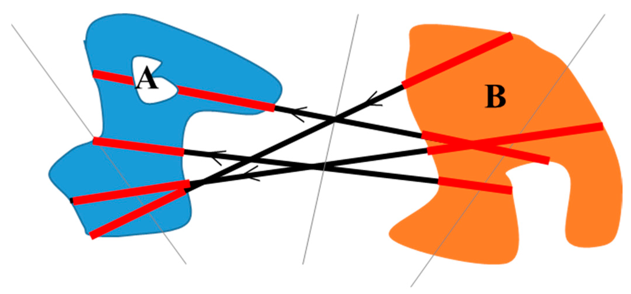
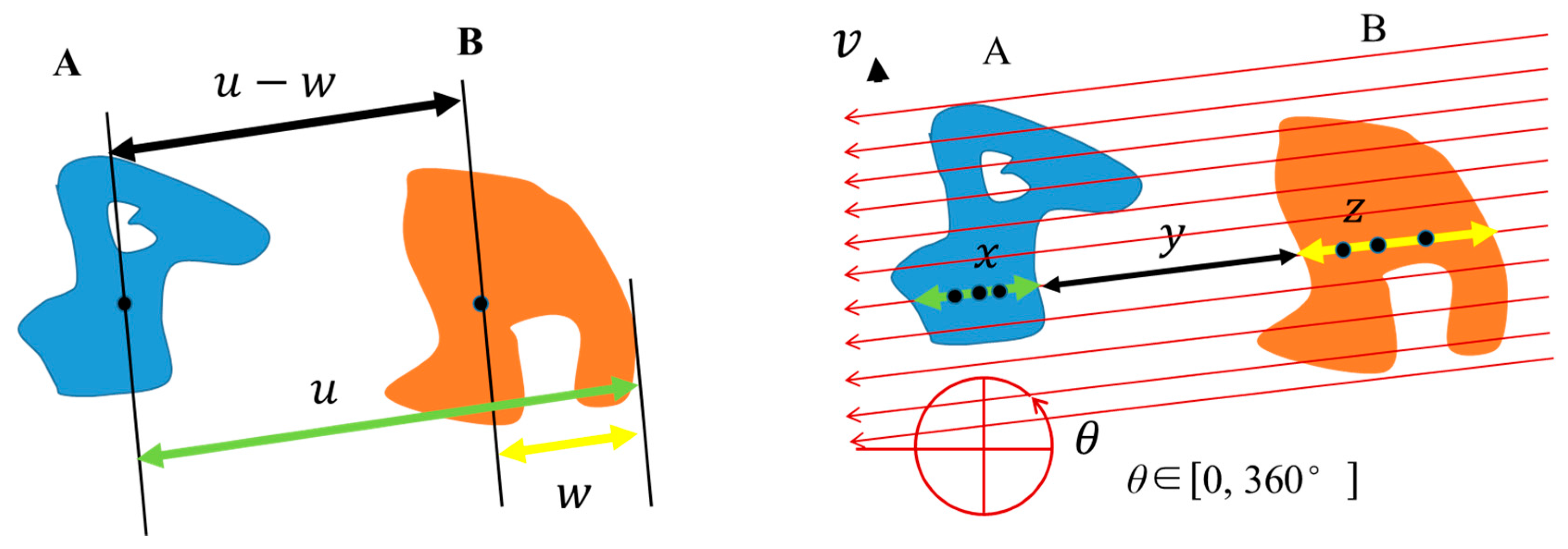
21]. Compared to methods based on geometric features, the histogram of force (
F-histogram) is sensitive to size, distance, shape, and direction, indirectly uniting the three types of position relations by calculating the force between two objects. The
F-histogram is also more convenient to obtain because it does not require the calculation of the boundary perimeter of the objects [
22,
23,
24,
25,
26,
27]. However, the
F-histogram is designed to acquire the position relations between pairwise objects [
28], and it is not suitable for modeling multiple objects in remote sensing images. In image indexing and retrieval, the
F-histogram has been extended to describe a group of objects located near the image center [
24,
25]. However, this method needs two reference objects placed outside the circumcircle of the group of objects.
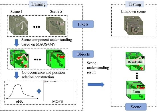
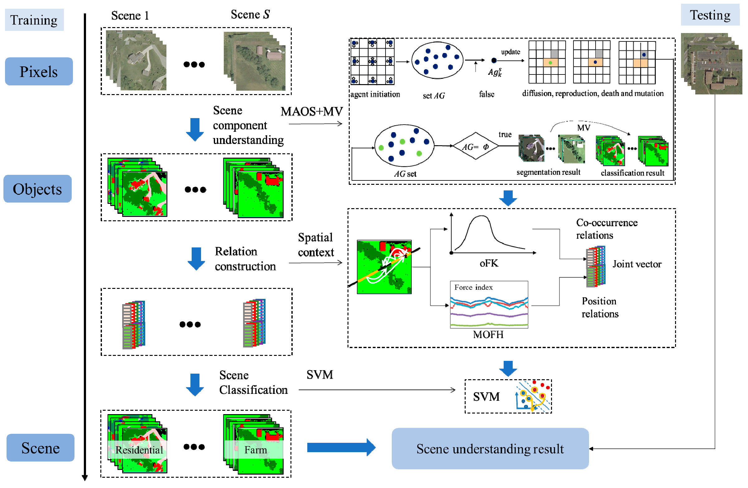
In this paper, to solve the problem of scene understanding, a bottom-up scene understanding framework based on the multi-object spatial context relationship model (MOSCRF) is proposed to bridge the semantic gap between pixels and the high-level semantics of HRSIs scene understanding. MOSCRF abides by a bottom-up sequence of pixels-objects-scenes, making it easy to parse the image hierarchically. In MOSCRF, the scene understanding includes three parts: (1) object-oriented classification; (2) construction of the co-occurrence relations and position relations; and (3) scene sematic category understanding.
The contributions of this paper are as follows:
- (1)
MOSCRF is used to understand the scene components and their co-occurrence relations and position relations. When determining the scene, MOSCRF takes advantage of the complementary nature of the fisher kernel coding of objects (oFK) and the multi-object force histogram (MOFH) to dissect the scene from two different aspects. The oFK is concerned more about the co-occurrence relations of different objects, whereas the MOFH pays more attention to the spatial distribution of the scene.
- (2)
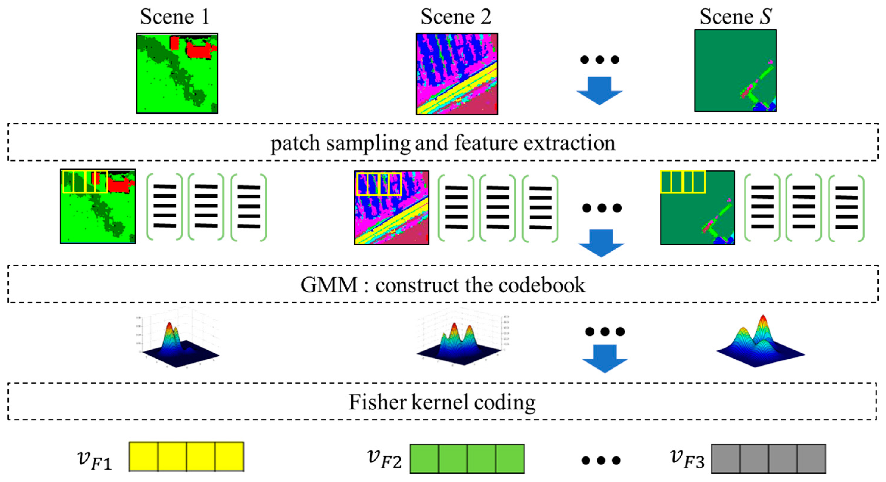
The oFK is used to model the co-occurrence relations by introducing the fisher kernel coding to objects. Compared to the traditional methods, the oFK is a compact, low-dimensional and refined representation of the distribution of objects categories by using a gradient vector.
- (3)
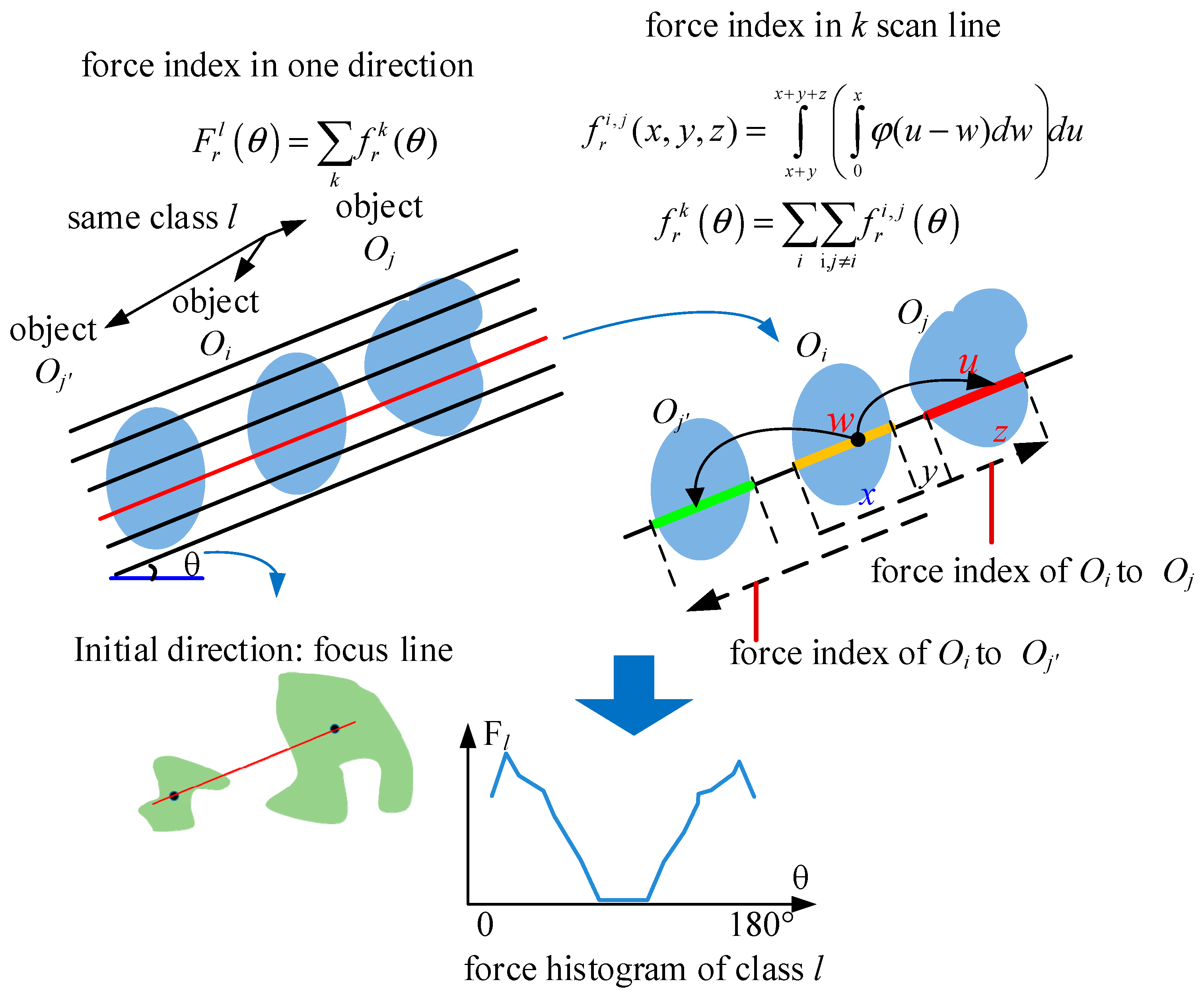
The MOFH is used to model the position relations for multiple objects. Aimed at dealing with the multiple objects in HRSIs, the MOFH adds a global scan line strategy and a rollback strategy to the traditional F-histogram. To keep the invariance to rotation and mirroring, the initial direction is defined as the centroid line between the object with the biggest area and the object with the smallest area. Finally, the feature is the mean and standard deviation of the MOFH curve. The MOFH explains the interaction of the internal objects in different directions.
The remainder of this paper is organized as follows.
Section 2 introduces the basic theory of the fisher kernel coding (FK) and
F-histogram.
Section 3 describes the MOSCRF construction procedure. The experimental results are reported in
Section 4, followed by the sensitivity analyses in
Section 5. Finally, the conclusions are provided in
Section 6.
4. Experiments and Analysis
To test the performance of the proposed MOSCRF, three datasets with progressive levels of complexity were put into use: a synthetic dataset, a USGS dataset, and the Wuhan IKONOS dataset. The synthetic dataset was used to verify the spatial layout through a visual inspection. The other two datasets were used to test the classification accuracy of MOSCRF.
In the step of object-oriented classification, the features were the spectral feature and the homogeneity of the gray-level co-occurrence matrix (GLCM) feature, and the classifier was SVM with radial basis function (RBF) kernel. The parameters of SVM were obtained by five-fold cross-validation. MAOS and MV were combined to restrict the result. The scale of the segmentation was 20 and the number of initial agents was 2000. In the step of scene sematic category understanding, we compared methods based on visual words of low-level features, such as the BoVW, spatial pyramid match (SPM), LDA and FK, methods based on deep learning features such as CNN, and methods based on objects such as frequency vector and a pair of objects (FH2) with MOSCRF. Besides, we compared the performance of different classifiers like SVM, naive Bayesian (NB), k-Nearest Neighbor (kNN), random forest (RF), and artificial neural network (ANN) acting on MOSCRF. The overall accuracy (OA) was measured by the mean, along with the standard deviation. The consistency test is Wilcoxon test. The details of the experiments are as follows.
4.1. Experiment 1: Synthetic Dataset
The synthetic dataset is defined based on the Google dataset of SIRI-WHU [
6] (
http://rsidea.whu.edu.cn/resource_sharing.htm), including three types of scenes: residential, commercial, and industrial area (
Figure 6). The process of generating the synthetic is as follows. First, select five images randomly from the Google dataset. Second, divide the images into building, road, tree, and other land-cover classes by artificial annotation. Third, rotate each image 90°, 180°, and 270° to generate other images. Fourth, flip all images in the horizontal and vertical directions to acquire the remaining images. Consequently, the synthetic dataset consists of 120 images and each scene contains 40 images.
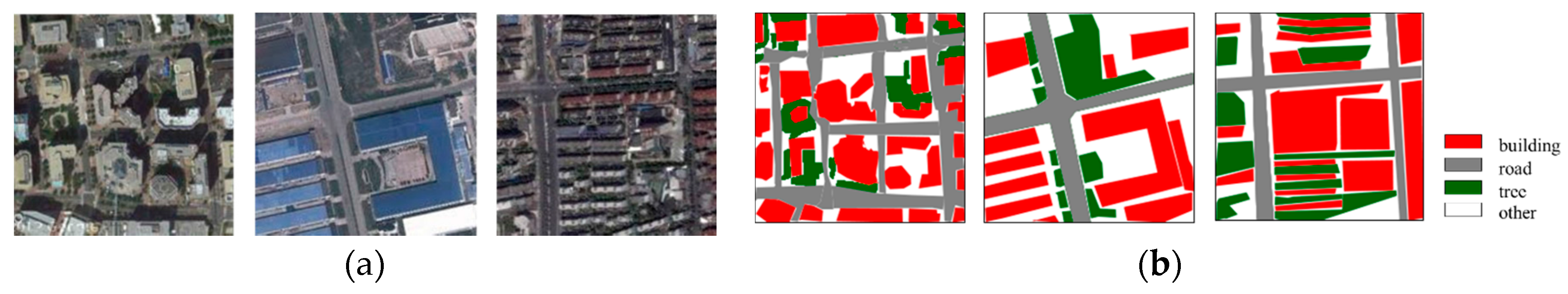
Figure 7 shows the visual result. From left to right in
Figure 7a are the initial image, its rotation, its mirror.
Figure 7b is the MOFH. From top to bottom, the scene categories are commercial, commercial, industrial, industrial, residential, and residential. Since the horizontal three images have the same force histogram, they are represented by a graph. According to the transverse comparison, it is easy to see the invariance to rotation and mirroring of the MOFH. According to the vertical comparison, it is clear that the different scenes have different spatial configurations.
4.2. Experiment 2: USGS Dataset
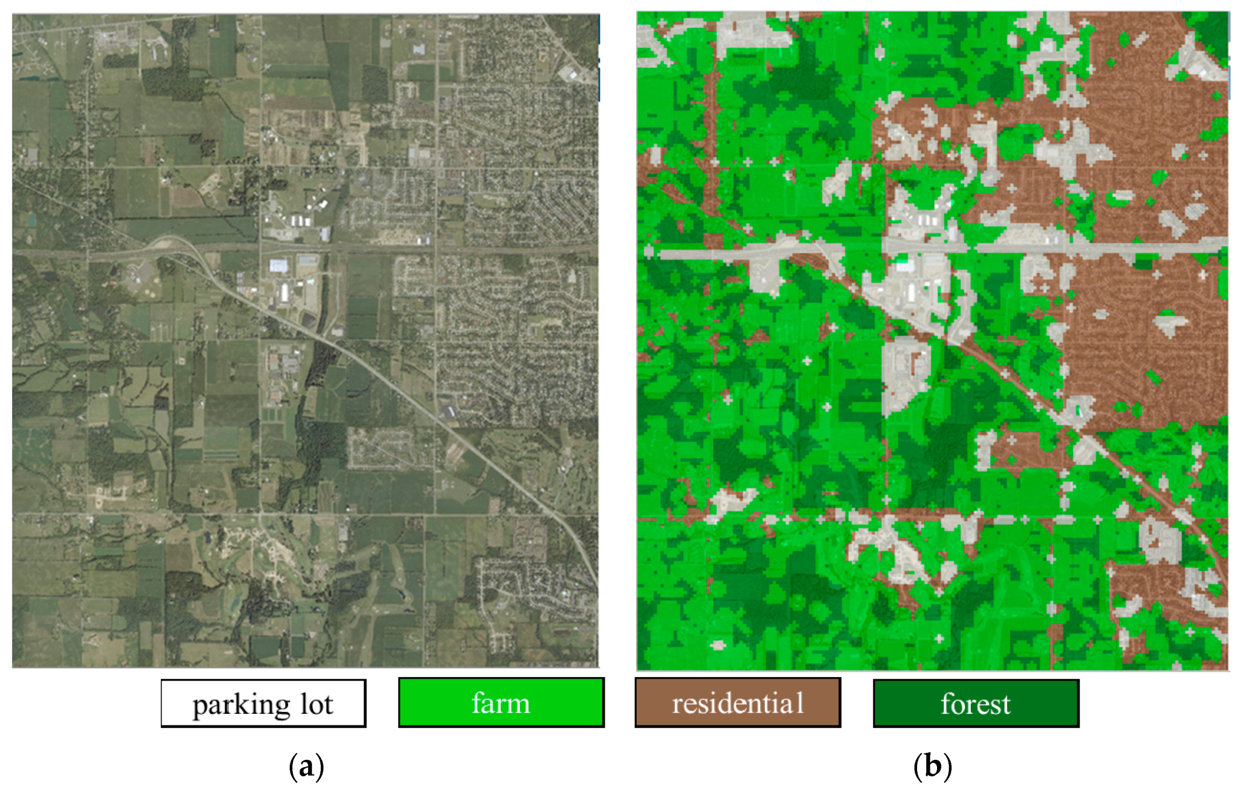
The USGS dataset was generated from a USGS database of Montgomery, Ohio, and contains a large image (
Figure 8a) with the size of 10,000 × 9000 pixels and four scene classes of residential, farm, forest, and parking lot, with 143, 133, 100, and 139 images, respectively (
Figure 9). For all the images, the size was 150 × 150 pixels and the resolution was 0.61 m. In these scenes, the objects were divided into five land-cover classes, namely, water, grass, tree, road, and building, whose numbers of samples were 208,299, 637,054, 594,930, 304,919, and 246,824, respectively.
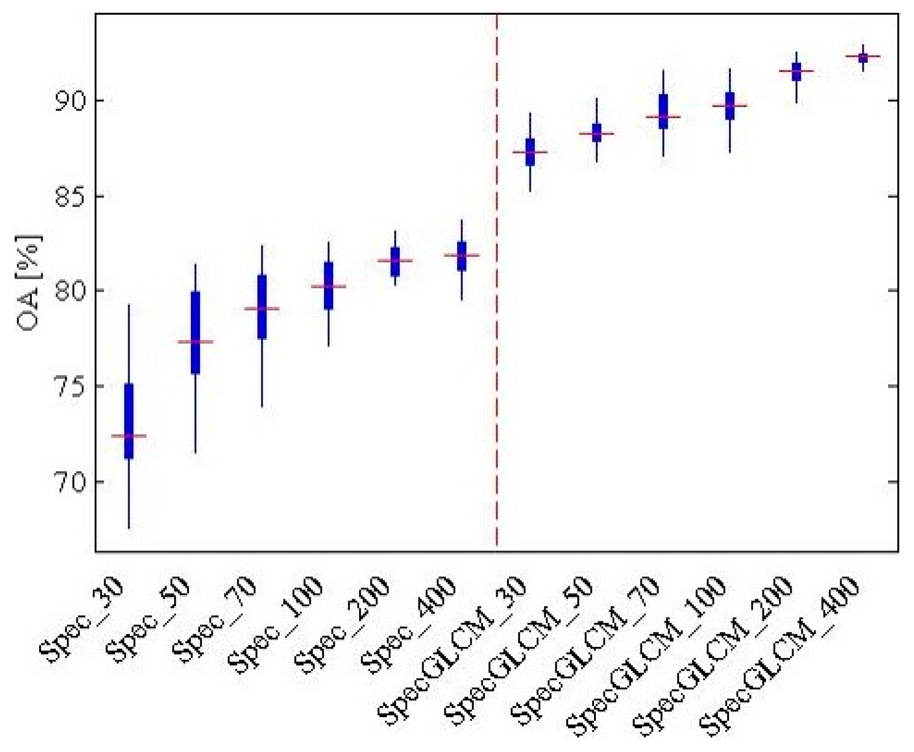
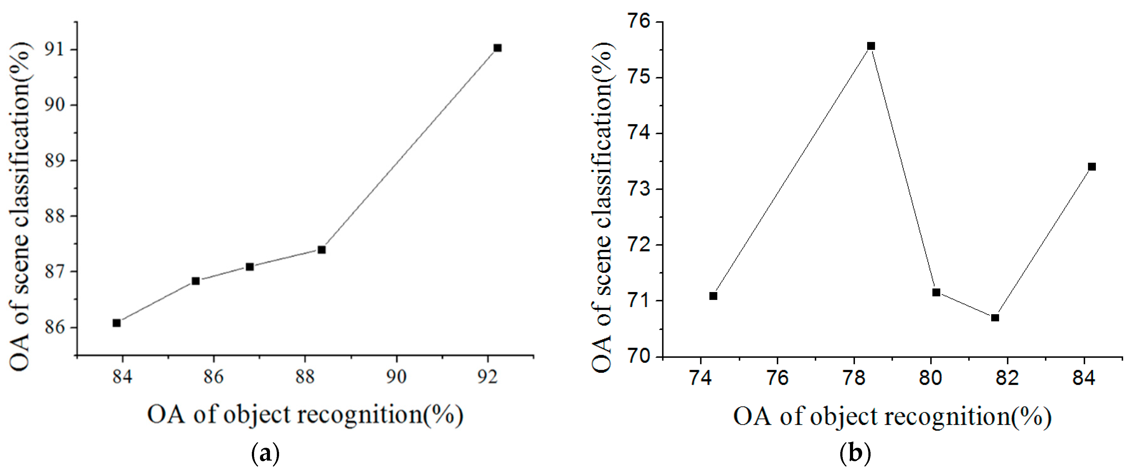
For the object-oriented classification, the accuracies of the land-cover classification with the different types of features and different numbers of training samples are shown in
Figure 10. It can be seen that it is better to use the spectral feature and the GLCM for the USGS dataset, as the OA is generally higher than when just using the spectral feature. The OA increases rapidly at first and then tends to stabilize with the increase of the training samples. The best OA, 92.2%, is obtained with 400 training samples in each class, which is the same as the Wuhan IKONOS dataset. Therefore, for the land-cover classification, the low-level feature was the combination of the spectral feature and the GLCM. The number of training samples was 400 in each class of land cover.
For oFK, the patch size was 8, the grid spacing was 4, and the number of cluster center was 32. For MOFH,
of MOSCRF was set to 3°, and
r was chosen as 0.5. The force indices were then from 60 different directions. SVM classifiers with RBF kernel were selected. The penalty factor and the bandwidth coefficient were tested by three-fold cross-validation. In the process of scene sematic category understanding, 50 images in every scene class were randomly selected as training samples, and the process was repeated 100 times. The accuracies of the scene understanding are listed in
Table 1. The accuracies of MOSCRF based on different classifiers are listed in
Table 2.
In
Table 1, it can be seen that, compared to traditional methods based on objects, MOSCRF has the highest accuracy of 92.73%; it especially has an improvement of about 17% compared to frequency vector. When the dataset is relatively small, the performance of MOSCRF exceeds the simple CNN about 5%. Although MOSCRF is lower than methods based on visual words of low-level features, it considers the distribution of internal components of the scene and is more in line with people’s understanding of the scene. In
Table 2, it is obvious SVM performs best, followed by ANN, and NB performs worst. The
p-values of all classifiers are bigger than 0.05, reflecting the classifier is efficient.
According to the confusion matrix in
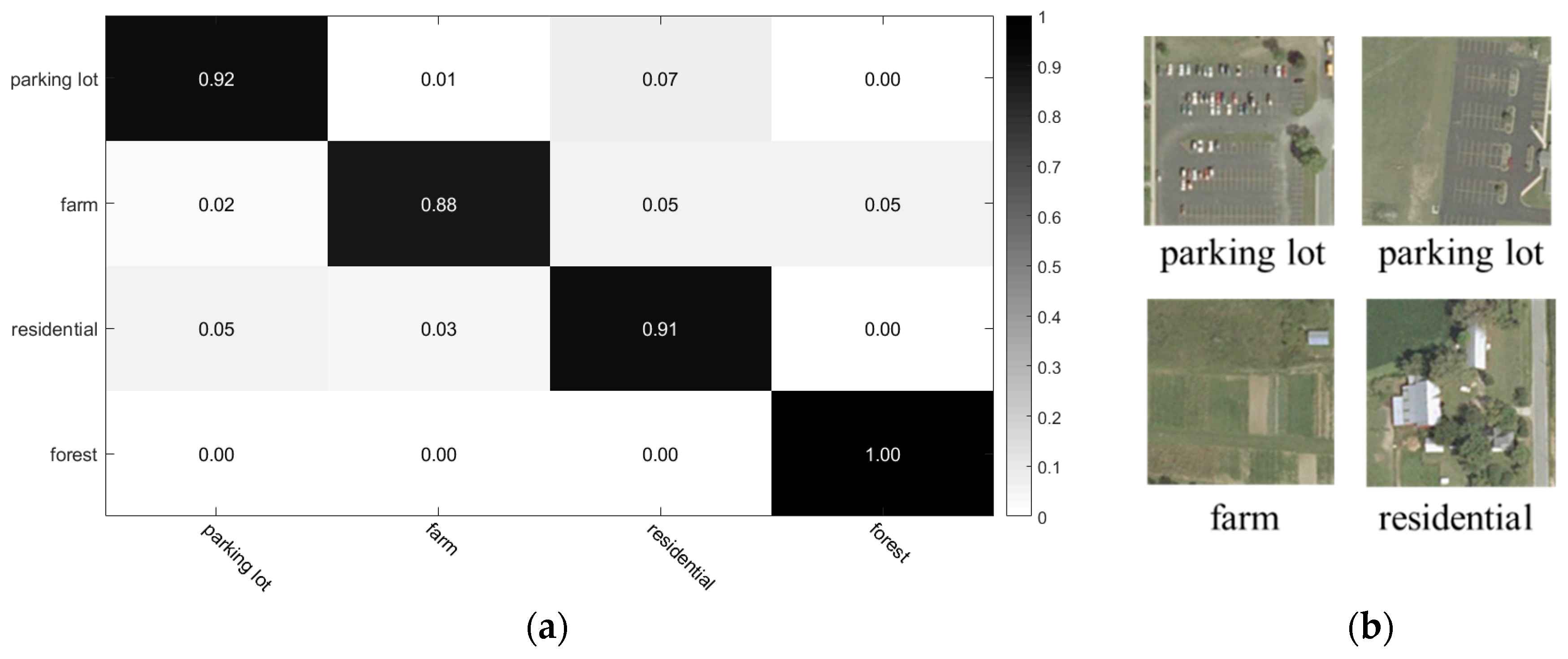
Figure 11a, MOSCRF performs the best in distinguishing the forest area with almost zero error. Though the number of test images of farm is smaller than residential area and parking lot, the misclassification is larger than other scene categories because the farm area contains cars, buildings and trees, leading to divide into residential and forest. The training ratio and accuracy of parking lot and residential is similar, meaning the recognizing ability of MOSCRF is similar, too.
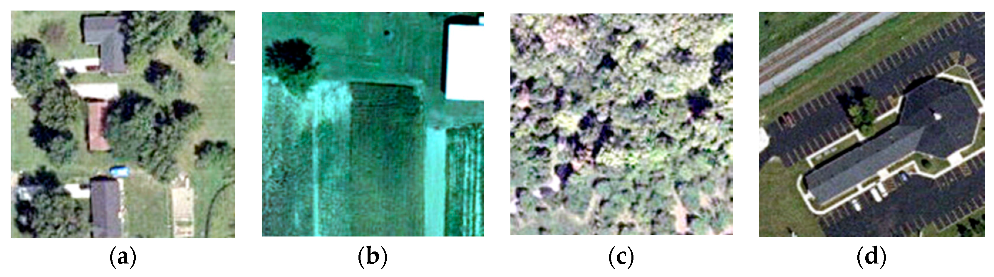
Figure 11b shows some of the images classified correctly by MOSCRF but incorrectly by frequency vector. It can be seen that both methods can classify the pure scenes such as forest, but MOSCRF has a better ability to recognize those scene categories with complex spatial configuration.
According to
Figure 8b, we can see that the Montgomery area is covered by water, grass, trees, roads, and buildings, with farm being the commonest scene class. Parking lots are found at the sides of the roads, and the residential area is to the northeast and east. Parking lots are obviously more common in the residential area.
4.3. Experiment 3: Wuhan IKONOS Dataset
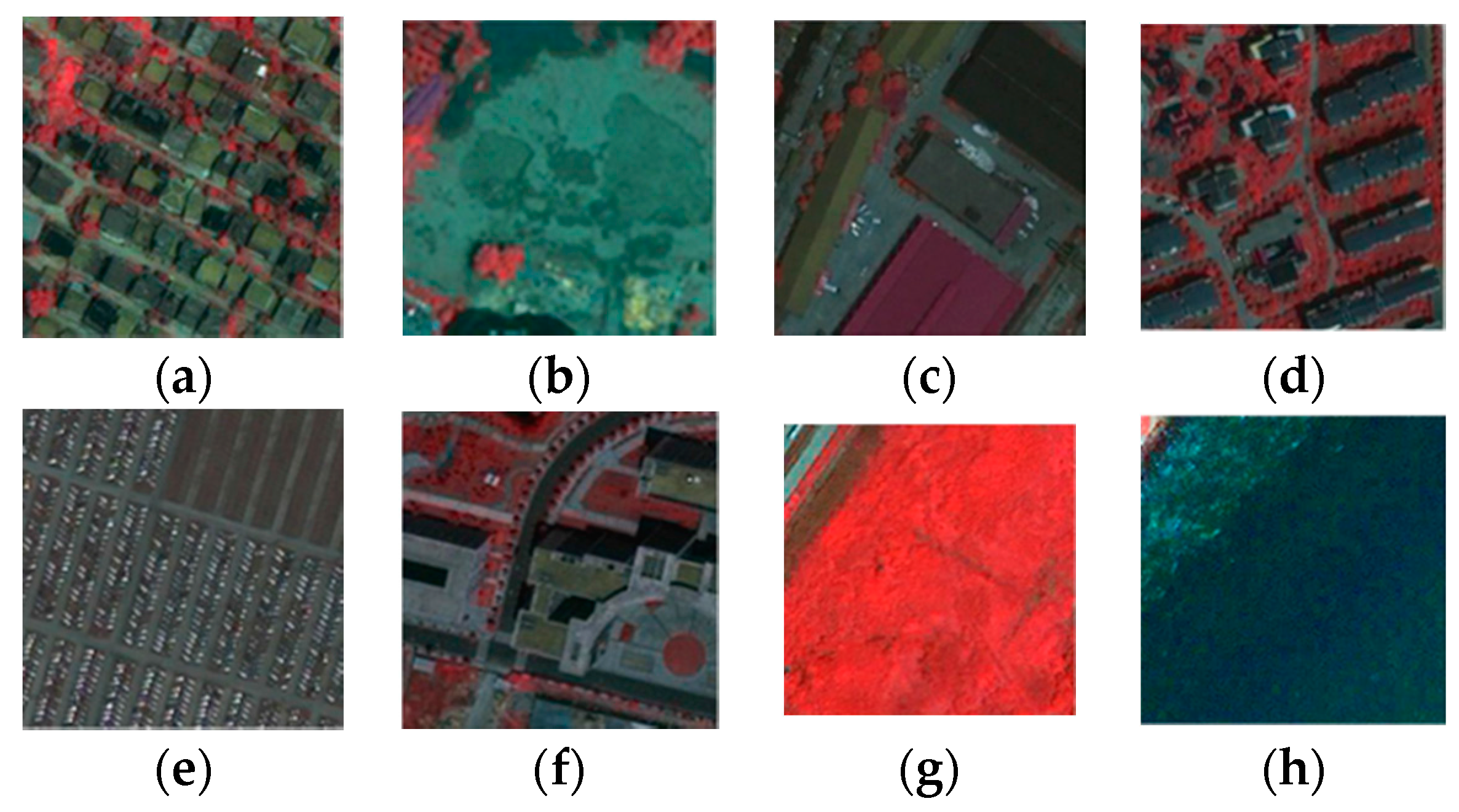
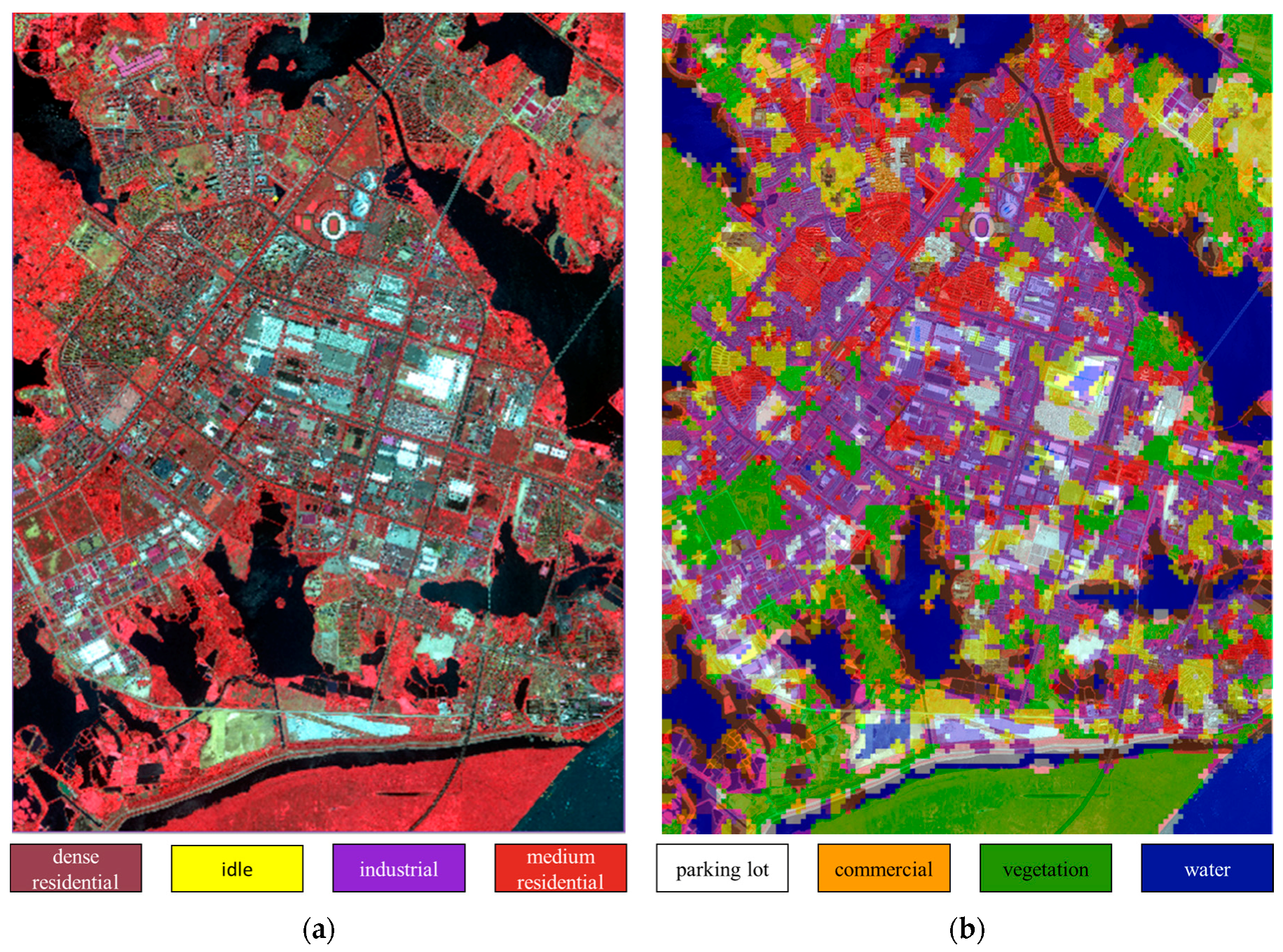
The third dataset is the IKONOS images of the Wuhan Hanyang district obtained in 2009, including a large image (
Figure 12a) with the size of 6150 × 8250 pixels and eight scene classes: dense residential, idle land, industrial, medium residential, parking lot, commercial district, vegetation, and water (
Figure 13). Each scene includes 30 images with the size of 150 × 150 pixels and a 1 m resolution. The objects are divided into nine land-cover classes, including three types of buildings, three types of roads, vegetation, water, and soil, with 23,637, 46,307, 118,710, 118,238, 119,392, 22,996, 89,955, 102,614, and 13,006 samples, respectively.
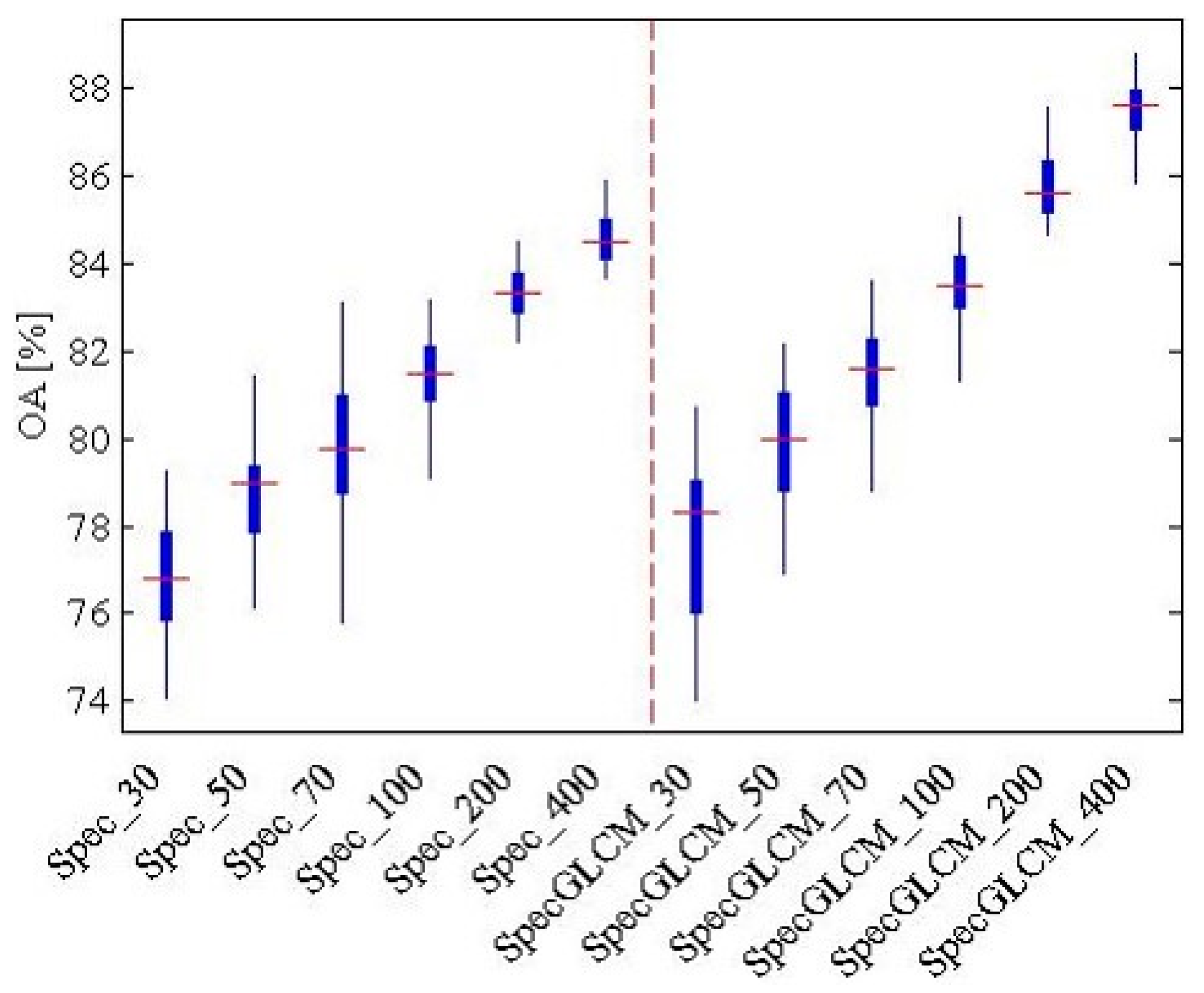
In
Figure 14, for the Wuhan IKONOS dataset, it can be seen that it is more valid to use joint features (i.e., the spectral feature and the GLCM) than just the spectral feature when the number of training samples ranges from 30 to 400. The best accuracy, 87.5%, is acquired when there are 400 training samples and the features are joint features. The land-cover recognition result with the highest accuracy was then used in the subsequent scene sematic category understanding.
In this case, 80% of the images in every scene class were randomly selected as training samples. The other parameters of the relation construction and scene sematic category understanding were the same as in the USGS dataset.
Table 3 lists the accuracies of the different methods.
In
Table 3, it can be seen that the performance is different from the USGS dataset. Here, MOSCRF acquires the best accuracy, 80.63%, which is at least 3% higher than the other methods. Comparing CNN to MOSCRF explains that MOSCRF is more suitable when lacking training samples, while comparing FK or LDA to MOSCRF reflects that ground object information is useful to scene classification. That is, the relations of objects are helpful in scene understanding. Both co-occurrence relations and positions relations are essential in scene understanding, according to the result that MOSCRF is 7% higher than frequency vector and FH2. In
Table 4, all classifiers are usable, while SVM is the best, followed by RF. NB is the worst and is nearly 20% lower than SVM.
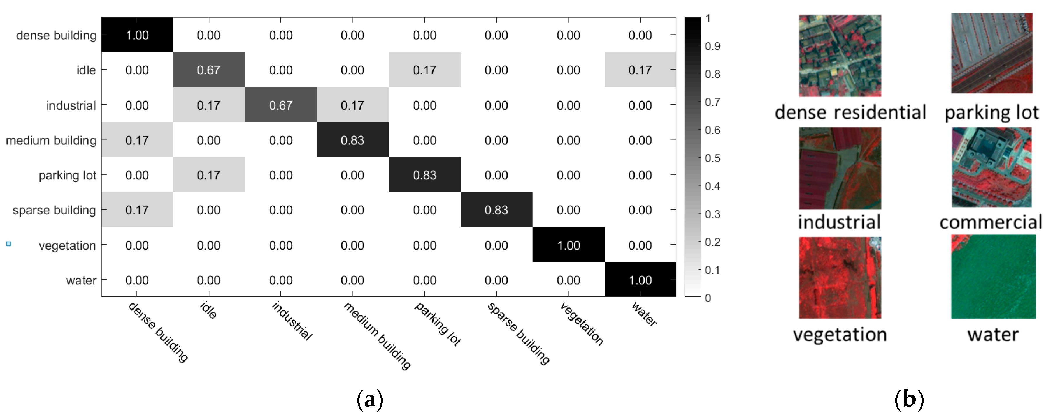
According to the confusion matrix in
Figure 15a, MOSCRF performs the best in distinguishing dense building, vegetation and water because of their regular distribution and relatively pure objects. Meanwhile, the idle and industrial scene classes are difficult to distinguish because of the vague and similar spatial configurations of their internal components: roads, buildings, and soil.
Figure 15b shows some of the images that are classified correctly by MOSCRF but incorrectly by frequency vector. It can be seen that MOSCRF is good at recognizing those objects with similar area proportions but different spatial configurations.
In
Figure 12b, we can see that the land-cover types are complex in Hanyang, including three types of buildings, three types of roads, vegetation, water, and soil. The area is still developing and the city planning is incomplete. As a result, the spatial layout of Hanyang is not regular.
6. Conclusions
Although BoVW, topic models, and deep learning algorithms can acquire a relatively high accuracy in scene classification, they do not take the prior knowledge of the objects into consideration. Therefore, they cannot fully understand the components of the images and their relations in the scene. In this paper, to solve this problem, we have proposed scene understanding based on the spatial context relations of multiple objects. The proposed approach consists of three main steps: (1) object-oriented classification based on MAOS + MV; (2) spatial context relations construction consisting of co-occurrence relations construction by the oFK and position relations construction by the MOFH; and (3) scene sematic category understanding by SVM-RBF. The oFK is the extension of the traditional FK based on low-level features in replacing the low-level features with the category information to justify the distribution of the object categories. MOFH extends the F-histogram of pairwise objects into multiple objects to serve the HRSIs and express the spatial layout of the scene. Moreover, the proposed MOFH has the characteristics of invariance to rotation and mirroring. MOSCRF is the framework of scene understanding based on these three steps.
The experimental results not only show that the proposed method performs better with than the traditional methods and classifiers, but it also identifies the internal composition of the scene and the relations of the objects. Therefore, MOSCRF has clear geographical significance in researching the internal patterns of scenes and is very deserving of further study to mine more information and improve the accuracy of scene understanding.


