Examining Multi-Legend Change Detection in Amazon with Pixel and Region Based Methods

Abstract

Post-classification comparison is one of the most widely used change detection methods. However, it presents several operational problems that are often ignored, such as the occurrence of impossible transitions, difficulties in accuracy assessment and results not accurate enough for the purpose. This work aims to evaluate post-classification comparison change detection results obtained from LANDSAT5/TM data in a region of the Brazilian Amazon, using three legends in different levels of detail and both pixel wise and region based classifiers. A distinctive characteristic of the used approach is that each change mapping is the result of the combination of 100 land cover classifications for each date, obtained using varied training samples. This approach allowed to account for the training samples choice into the methodology, as well as the construction of confidence mappings. We presented and discussed different approaches for evaluating change results, such as the likelihood of land cover transitions occurring within the study area and time gap, the use of rectangular matrices to incorporate the occurrence of impossible or non evaluable changes and classification uncertainty. In general, change mappings obtained from region based classifications showed better results than the ones obtained from pixel based classifications. Globally, the use of region based approaches, in contrast to pixel based ones, led to an increase in accuracy of 15.5% for the change mapping from the most detailed legend, 7.8% for the one with the legend with intermediate level of detail and 3.6% for the less detailed one. In addition, individual transitions between land cover classes were better identified using region based approaches, with the exception of transitions from a non agriculture class to an agricultural one. The proposed quality mappings are useful to help to evaluate the change mappings, mainly in legend levels with higher level of detail and if reference samples are unreliable or unavailable. It was possible to access, in a spatially explicit way, that at least 29.0% of the pixel based change mapping and 21.9% of the region based one from the most detailed legend were erroneous classified, without ground truth information on the evaluated date. These values decreased to 0.5% and 1.4% (respectively the pixel and region based approaches) for results with the legend with the intermediate level of detail and are non existent in the results from the less detailed legend. The more generalized the legend (lower number of classes), the most similar are the accuracy of region and pixel based change mappings. These accuracy values also increase as fewer classes are considered in the legend, since similar classes are assembled during clustering, which reduces the overlap between groups. However, this accuracy is still low for operational purposes in areas with few changes, even considering the very high accuracy of the land cover classifications used to generate the change mappings (land cover classification with Overall Accuracy higher than 0.98 resulted in change mappings with Overall Accuracy around 0.83).

1. Introduction

Change detection is the process of identifying differences in the state of an object or phenomenon at distinct times [1]. Change detection studies contribute to the understanding of ecosystems over time and also of natural phenomena as well as human activities [2]. Since the first overviews regarding change detection in the 1960s [3], many works in this discipline have been conducted using remote sensing data. Among the recent works, we can cite the monitoring of arid environments [4], shorelines [5] and forests or woodlands [6,7,8,9] as well as detection of urban expansion [10], changes in buildings structure [11], changes in submerged sea grass biomass [12], mapping of landslides [13], damage to cultural heritage sites [14] and the proposition of new methodologies [15,16,17,18,19].

In order to select suitable data and methodology for change detection, it is essential to fully determine the kind of change to be detected. Firstly, it is important to differentiate between ‘land cover’ and ‘land use’. Land cover refers to the biophysical state of the earth surface. This description includes the amount and type of vegetation, water and other materials and structures of natural or anthropogenic origin. Land use involves both biophysical attributes as the activities carried out and the manipulation intention, namely the purpose for which the land is used for human interest activities [2,20]. Satellite image analysis enables the direct recognition of land cover. Land use is usually assigned by the analyst, based on the knowledge of the area, field data, other ancillary data or the land cover itself [20]. In addition, there are two major types of land cover changes: conversion and modification [2,20]. Conversion can be defined as the complete removal of a type of cover, to be replaced by another. Modification consists of more subtle changes that alter the land cover characteristics without changing its overall classification. Note that the final stage of a modification process may result into conversion [20]. Changes can also be categorized as binary (change/no change), detailed ‘from-to’ change trajectories, specific change types (e.g., deforestation, urbanization, agricultural expansion), or continuous variable change (forest disturbance and other changes resulting from modifications) [21]. To determine which types of change should be detected, it is important to select which kind of data and change detection methods should be used. For example, it is clear that a data set not sensitive to small changes would never offer satisfactory results for continuous variable change studies, or that methods which produce change/no change maps are not enough for specific change types studies.

According to [22], “the direct comparison of satellite derived land cover maps is one of the most established and widely used change detection methods”. This change detection methodology is also known as post-classification comparison. Since classifying a remote sensing image for land cover classification is a relatively well-known practice and the understanding of a class in one time is obviously easier than analyzing the trajectory of classes along time, it seems natural to use the post-classification comparison method for the initial analysis of land cover change in a given area. However, the accuracy of the final change map depends on the quality of each individual classification [2,22,23]. In particular, errors in the individual maps are additive in the combination (change mapping). Moreover, it is not possible to measure changes occurring in a lower scale than the combined errors of the individual maps [23] and since errors occur in the individual classifications, it is also possible that changes that could never actually occur in the field are registered [24]. According to [23], these issues are often ignored.

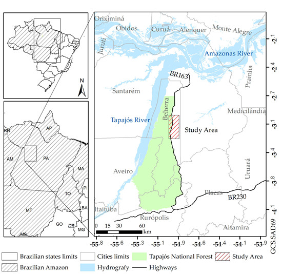
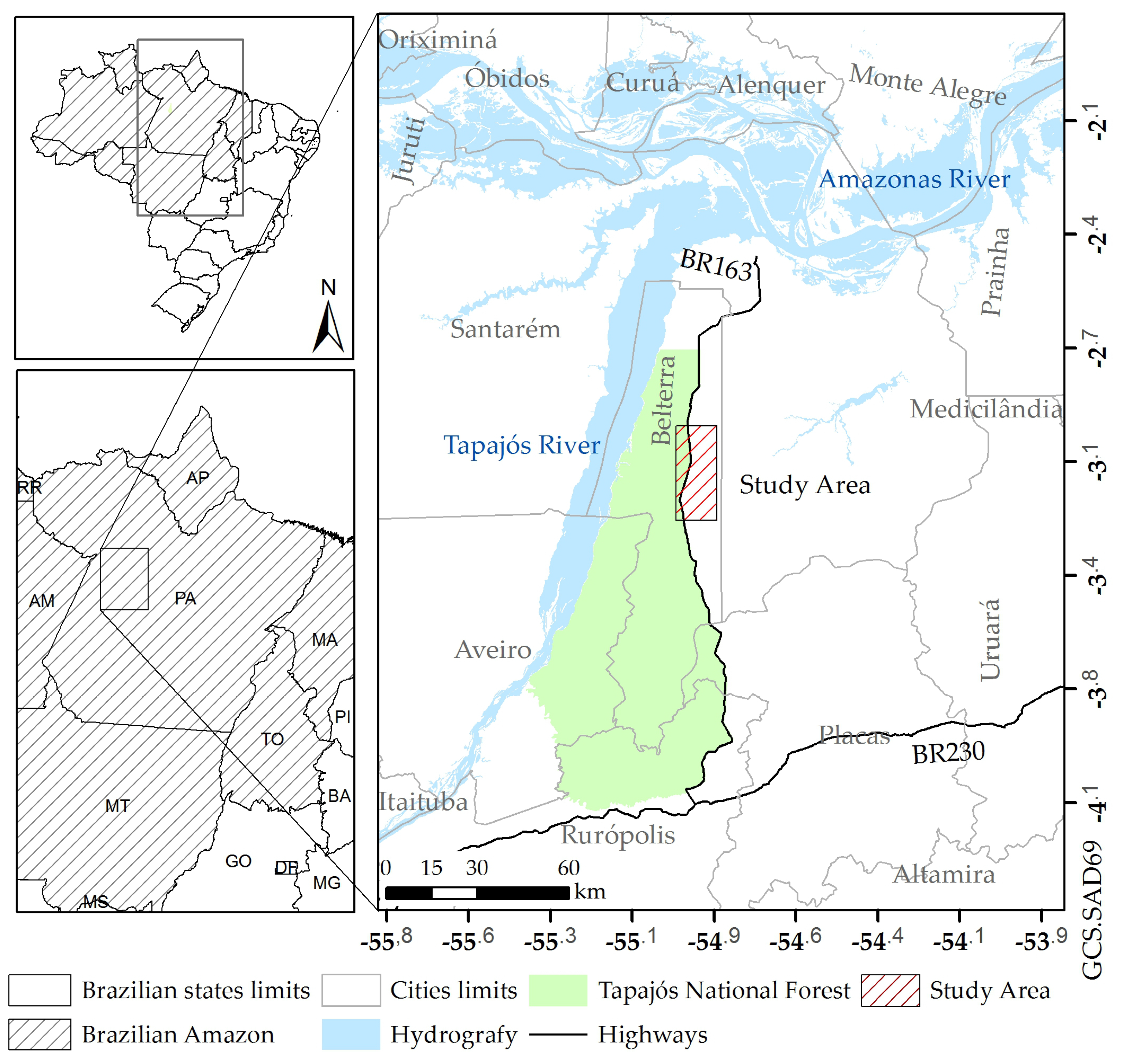
Due the need for more rigorous analysis considering change detection studies using post- classification comparison, this work aims to present a multi-legend change detection study in the Brazilian Amazon. Of particular interest within this work is to determine how the change detection process is affected by the detail level of the original land cover classifications. Change detection was conducted using both pixel and region based classification, considering legends with three different levels of detail. As a secondary objective, a methodology to improve post-classification comparison change detection by indicating impossible or not expected changes is also presented. Two quality maps associated to the change mapping are also proposed, to better evaluate the results.

This paper is organized as follows. The studied area, field information and imagery used are described in Section 2. Methods are explained in Section 3. The obtained results are presented in Section 4 and discussed in Section 5. Some final considerations and proposal of future works are made in Section 6.

2. Materials

2.1. Study Area and Field Information

This study focuses on detecting and identifying changes that occurred between June of 2008 and June of 2010 in an area of approximately 412 km² in Belterra, Pará state, located in the Brazilian Amazon. This area is illustrated in Figure 1, with geographical references. This region presents humid tropical climate, with average annual temperature at 25 °C, varying less than 5 °C throughout the year. Average annual precipitation is around 1820 mm, with higher precipitations usually occurring from January to May [25]. It is a relatively plane area and presents dense forest vegetation, in which woody lianas, palms and epiphytes are found. The study area presents patches of secondary vegetation, pasture and agriculture within the forest matrix. In addition, there are reports of logging, mining, hunting, fishing and inadequate use of fire in this region [25]. Considering land cover, this is a very heterogeneous area, in which both subtle and obvious changes occur over time. This area and time period was selected due to the availability of field data information within the proximate date, which allows for a more rigorous evaluation of the results.

Land cover classes were defined using field data information available from 2009 and 2010, as well as data from the Programme for the Estimation of Deforestation in Brazilian Amazon (PRODES) and the Land Use and Land Cover mapping of Deforested Areas in Legal Amazon Project (TerraClass), both from the years of 2008 and 2010. Visual interpretation of LANDSAT5/Thematic Mapper (TM) and Earth-Observing (EO-1)/Advanced Land Imager (ALI) images from the area in the aforementioned years were also incorporated. Ten land cover classes were defined, as presented in

Table 1. Land cover classes definition.

Acronym	Class Name	Description
BS	Bare Ag. Soil	Agricultural areas that at the sensing time presented bare soil
IA	Idle Ag. Area	Fallow annual agriculture areas, that presents herbs in green or senescent state
CA	Cultivated Area	Culture being cultivated in the area at the sensing time
CP	Clean Pasture	Pasture areas, covered by gramineaes, in which invasive shrub plants can be found in less than 15% of the feature
OP	Overgrown Pasture	Pasture areas in which invasive shrub plants are present in more than 15% of the feature
SV1	Initial S.V.	Areas of secondary vegetation (grown after completely razing the natural forest) formed predominantly by herbaceous vegetation and shrubs
SV2	Intermediate S.V.	Areas of secondary vegetation composed mainly by shrubs and small trees
SV3	Advanced S.V.	Areas of secondary vegetation, composed by trees with mean height of 20 m, with presence of emergent trees and, to a lesser extent, shrubs and herbaceous vegetation
MF	Modified Forest	Forested areas modified by logging and/or fire
MA	Mature Forest	Well structured, climax forests, with small to none evidence of alteration

Notes: Ag. = Agricultural; and S.V. = Secondary Vegetation.

. The name of land cover classes, the acronyms used and a brief description of each are presented in this table.

In this study, three legend levels were considered. This was done by the generalization of the legend that encompasses the ten described classes. According to [26], map generalization is the process that simplifies the representation of geographical data to produce a map at a certain scale with a defined and readable legend. Usually, to make a legend readable at a smaller scale, some objects are removed or enlarged, aggregated to another or displaced and all objects are simplified, as well as the information. In this study, generalization refers to class clustering processes, in which classes are merged to form a hierarchical legend. The merging of classes may increase the accuracy of the results [27,28,29]. In addition, the use of a hierarchical legend enables both multi scale studies and to harmonize local level studies to regional or global studies [30].

The ten identified land cover classes were organized to form three legends levels, as illustrated in Figure 2. In this figure, Li indicates the level, with i varying from 1 to 3. The L1 legend is the most detailed one, encompassing the ten land cover classes identified. The L2 legend was thought to be used in regional scale studies and is somewhat similar to legends used while working with low resolution images, in which basic land use (agriculture or pasture) and structure (sparsely or densely vegetated forests) were taken into account. The L3 legend separates only the two major groups of land cover classes presented in the work, namely, cultivated areas (agricultural areas and pasture) and natural or semi-natural areas (secondary vegetation and forests), similarly to the categories presented in the dichotomous phase of the Land Cover Classification System from the Food and Agriculture Organization (FAO) [31].

The three legend levels were generated to encompass different types of studies that may be expected regarding LULC change detection in the Amazon. Labeled samples from each land cover class encompassing L1 legend were collected and divided in two sets, training and test, as illustrated in Figure 3. In this figure, the collected samples are shown over band 5 of LANDSAT5/TM images from June of both 2008 and 2010, for localization, and the number of samples of each class is presented considering the original resolution of LANDSAT5/TM data (30 m). These samples were merged to form L2 and L3 training and test sets.

2.2. Remote Sensing Data

Two images from the TM sensor, on board of LANDSAT5 satellite, were used in this work. We opted to use this image since the data is well known, but this study could be conducted with similar types of data with few adjustments. The images used were sensed respectively on 23 June 2008 and 29 June 2010, both in path/row 227/62 with 30 m of spatial resolution, 8 bits and 7 spectral channels. These images were selected because of the low cloud coverage and similarities in phenology and atmospheric conditions. The LANDSAT5/TM images were obtained from INPE’s catalog [32], already projected to UTM-WGS84. The images were orthorectified using Shuttle Radar Topography Mission version 4 (SRTM4) data and the Rational Function Model (RFM) presented in PCI Geomatics 13.0 software [33], maintaining the 30 m of pixel size. A feature selection process was executed on bands 1 to 5 and 7 of LANDSAT5/TM data. This process used the minimum Jeffries-Matusita (JM) distance [34] between the training samples of all possible pairings of the ten described land cover classes from L1 legend.

We selected the set with three features for both data, due to small gains in JM distance for four features. Bands 2, 4 and 5 were selected for data pertaining to both dates, because this combination presented the highest minimum JM distance between the training samples of all possible pairs of classes from the most detailed legend (L1). These three selected bands will be reported as ‘TM’ in this work. This data is illustrated in Figure 4.

3. Methods

There are diverse categorizations of change detection methods presented in literature [2,22,35,36]. Tewkesbury et al. [22], for instance, separated the methodologies by the analysis units commonly used in remote sensing: pixel, kernel (a moving window), vector polygon, image object or hybrid. Considering similar methodologies within different analysis units, one major and common division may be amongst ‘layer arithmetic’, ‘post-classification comparison’, ‘direct classification’ and ‘hybrid methods’. In this work, we will consider as ‘layer arithmetic’ any method in which some kind of mathematical operation is calculated directly into the pixel values or derived features in order to detect changes. ‘Post-classification comparison’, as the name suggests, consists of classifying the data from each time separately and then comparing the resulting classifications. ‘Direct-classification’ consists in stacking the multi-temporal images and classifying it directly into multi-temporal classes (no change, specific changes or transitions), using supervised or unsupervised classification algorithms [22]. ‘Hybrid methods’ are those in which two or more types of change detection techniques are used together. The main advantages and disadvantages of each methodology are summarized in

Table 2. Main characteristics of change detection methods.

Technique	Advantages	Disadvantages
Layer arithmetic	Simple to implement, unnecessary previous knowledge of land cover changes, methods for analysis of mono-sensor change detection are well developed	Data from different dates must be calibrated/ radiometric corrected, difficulties in determining suitable data and thresholds, does not typify change (or no-change) classes
Post-classification comparison	Minimizes impacts of differences in radiometric characteristics, provides a complete matrix of change information, specific knowledge of changes is not necessary	Knowledge of land cover classes is needed for supervised approaches while unsupervised approaches may be complex to analyze, time and expertize needed regarding image classification, errors in individual classifications directly translated to the change map, possibility to register impossible types of changes, impossible to measure changes occurring in a lower scale than the combined errors of the individual classifications, difficulties in accuracy assessment
Direct classification	Only one classification stage is needed, effective to analyze time series, supervised approaches produce maps with only change/no-change classes of interest	Unsupervised approaches can provide results very complex to analyze, previous knowledge of existing change classes is needed for supervised approaches and training data sets can be very difficult to construct
Hybrid methods	Enables the use of results of different methodologies to facilitate/improve change detection	Expertise in different change detection methods needed, time consuming, skills in data manipulation and multiple software use may be necessary

[2,22,23]. As mentioned in Section 1, although post-classification comparison is widely used for change detection, it presents some problems that are often ignored. Thereby post-classification comparison was selected to be used in this study, because of its simplicity, common use and the necessity of explicit studies regarding the usefulness and accuracy of its results.

The more common methods to evaluate change detection accuracy are derived from the error matrix [2]. For binary maps, a 2 × 2 change/no change error matrix can be used [37,38], and indexes like prevalence, sensitivity, probability of false alarm and probability of detection calculated [38]. In [37], three variations of change/no change matrices are explained. For specific change classes, the use of traditional error matrix seems straightforward. The accuracy of transitions (from-to) can be estimated considering the transition error matrix [37], or change detection error matrix, as proposed by [39]. From post-classification comparison derived change mappings, evaluation can also be made through the accuracy assessment of the land cover classifications [23,37]. However, when considering post-classification comparison studies, one must remember the possibility of obtaining impossible changes or possible changes from which samples were not acquired. In [24], the authors proposed the use of rectangular error matrices, which table the reference samples and the classification, and calculated overall accuracy indexes over these matrices. In these matrices, impossible or unobserved changes were explicit. Another interesting approach was developed by Liu and Zhou [40], in which the authors determined the accuracy of trajectory changes by arguing change rationality with post-classification comparison. They created a set of rules regarding probability of changes from one class to another, based on the knowledge of the study area, and used it to separate ‘real changes’ from possible classification errors. A similar proposal can be seen in [41], in which the authors show a class transition matrix detailing the likelihood of transitions (likely, probable, possible and not likely) in order to refine and verify the quality of time series of land cover maps. Although this approach can be used without any labeled samples from a reference data, the joint application of the logical rules with matrices in which impossible changes are explicit can be useful for change detection results evaluation. A similar approach using both change class samples and a rules set of changes was used by [42] to compare SAR (Synthetic Aperture Radar) change detection results.

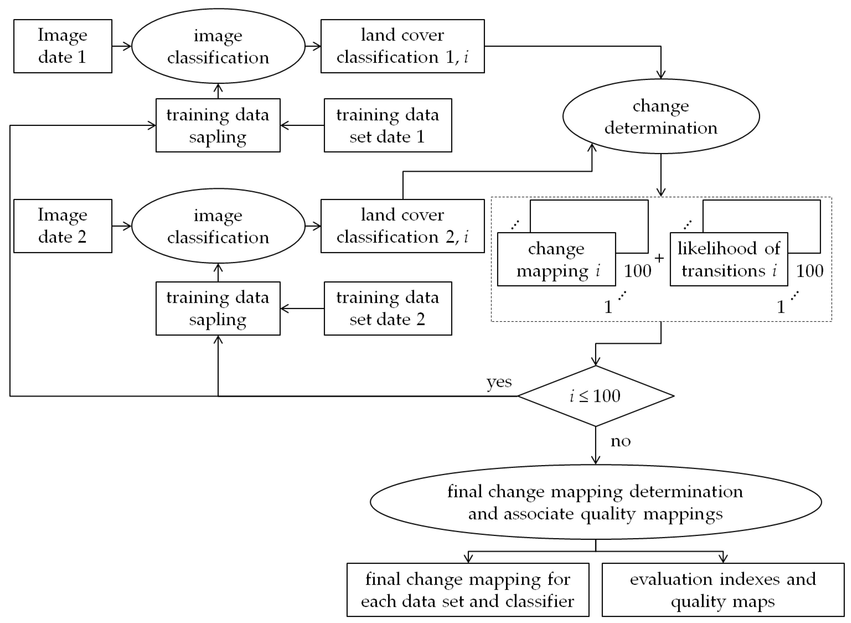
We used supervised classification, considering pixel and region-based classifiers. For each legend level and classifier, equally distributed sampled training data was used to produce a land cover classification for each date. This pair of land cover classifications was used to produce one change mapping with two pieces of information, herein the type of change and the likelihood of that transition occurring. This process was done 100 times, with the training samples being randomly selected again for each time, generating one set of 100 change mappings. From this set of change mappings, it was produced one final change mapping (with change type information) and two quality mappings: the likelihood of the transitions of the final change mappings and the uncertainty of the change determination process. These results were then evaluated. The general methodology is outlined in Figure 5 and detailed in the following subsections.

3.1. Image Classification

As previously mentioned, the TM data for the two dates was classified 100 times, using varied sets of training samples from each legend level and one given classifier. Two different classification approaches were analyzed in this work: pixel and region based. The classification procedure for each approach is described as follows.

3.1.1. Pixel Based Classification

We tested four supervised per pixel classifiers in this work: Maximum Likelihood (ML), k-nearest neighbor (K-NN), decision tree based J48 and support vector machine (SVM), as implemented in the packages Rasclass, RWeka and e1071, all for R software. ML was used considering Gaussian distribution. SVM was used with linear kernel in a ‘one-against-one’ approach. In order to select the optimum classifier to be used, we classified the TM data from 2010 using these classifiers in different parametrization and the most detailed legend level (L1—ten classes).

To each classification generated, the classifier was trained using 300 randomly selected pixels of each class, with replacement. This process was executed 100 times, generating 100 classifications for each classifier and configuration. Evaluation of classifications was also done using a Monte Carlo approach. For each classification, 100 confusion matrices and respective Overall Accuracy (OA) indexes were calculated, using 100 randomly selected pixels from the test set of samples, which results in 10,000 values of OA for each classifier. The mean value of these 10,000 OA were then compared using unpaired t-test with 1% of significance level. ML and SVM with cost = 1 achieved statistically similar mean OA results (0.73), which were statistically higher than the others mean OA values. Since ML is a well known classifier and simpler to use (no parameter tuning needed) than SVM, it was selected to classify the TM data for both dates and the three legend levels, considering the same Monte Carlo approach for the aforementioned sets of 100 classifications for each date and legend.

3.1.2. Region Based Classification

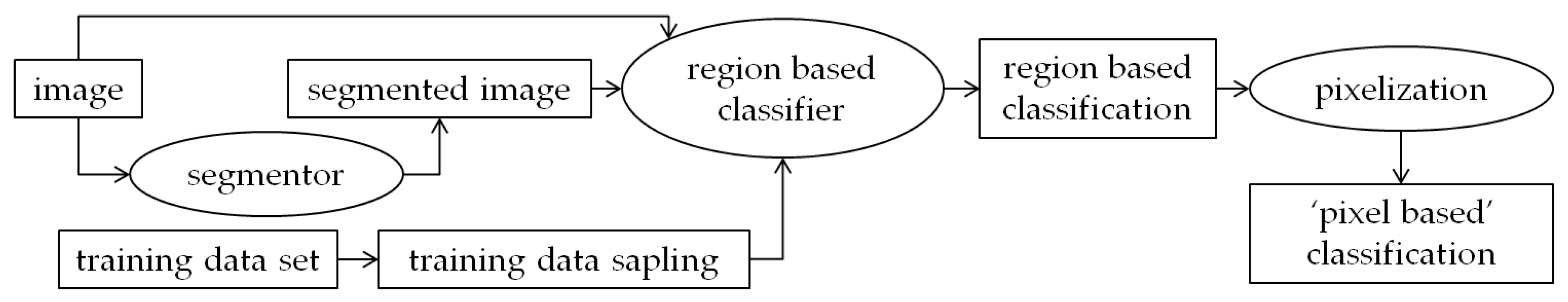
For region based classification, Minimum Bhattacharyya Distance classifier (B), as implemented in [43], was used. The steps necessary for generating a region-based classification with this classifier are illustrated in Figure 6. As can be seen, one segmented image is necessary for the process, and its construction is an important part of region based classification process [36].

The data sets from 2010 were segmented using several parametrization for four algorithms: Region Growing, implemented in TerraPixel [44]; the Watershed based segmentor implemented in Idrisi Selva [45]; Multiresolution Segmentation implemented in eCognition 8.0 [46] and MultiSeg [47]. We used both visual analysis and values of the Weighted Index for Segmentation Evaluation [48] to select the segmented image for use. The selected parametrization for 2010 data was also used for 2008 data, with good results. Multiresolution Segmentation algorithm from eCognition 8.0 software was selected, with the parameters Shape = Compactness = 0.3 and Scale = 30 to be used. In the resulting segmented images, areas with less than 100 pixels were grouped with those that shared the longest border with them, in order to enable the correct calculation of the Bhattacharyya Distance. It must be highlighted that similar results for other satellite images could be found by tuning the used parameters.

The Bhattacharyya Distance between the pixels in each segment and samples of each class was then calculated, and the class that resulted in the minimum distance is attributed to that segment. These segments were then pixelated to square pixels of 30 m, and used to produce the change mappings. In accordance with the methodology used for pixel wise classification, 100 classifications using B classifier were computed, using 300 randomly selected pixels for each class from the training set, in each date and legend level, with variation of selected pixels for each classification.

3.2. Change Determination

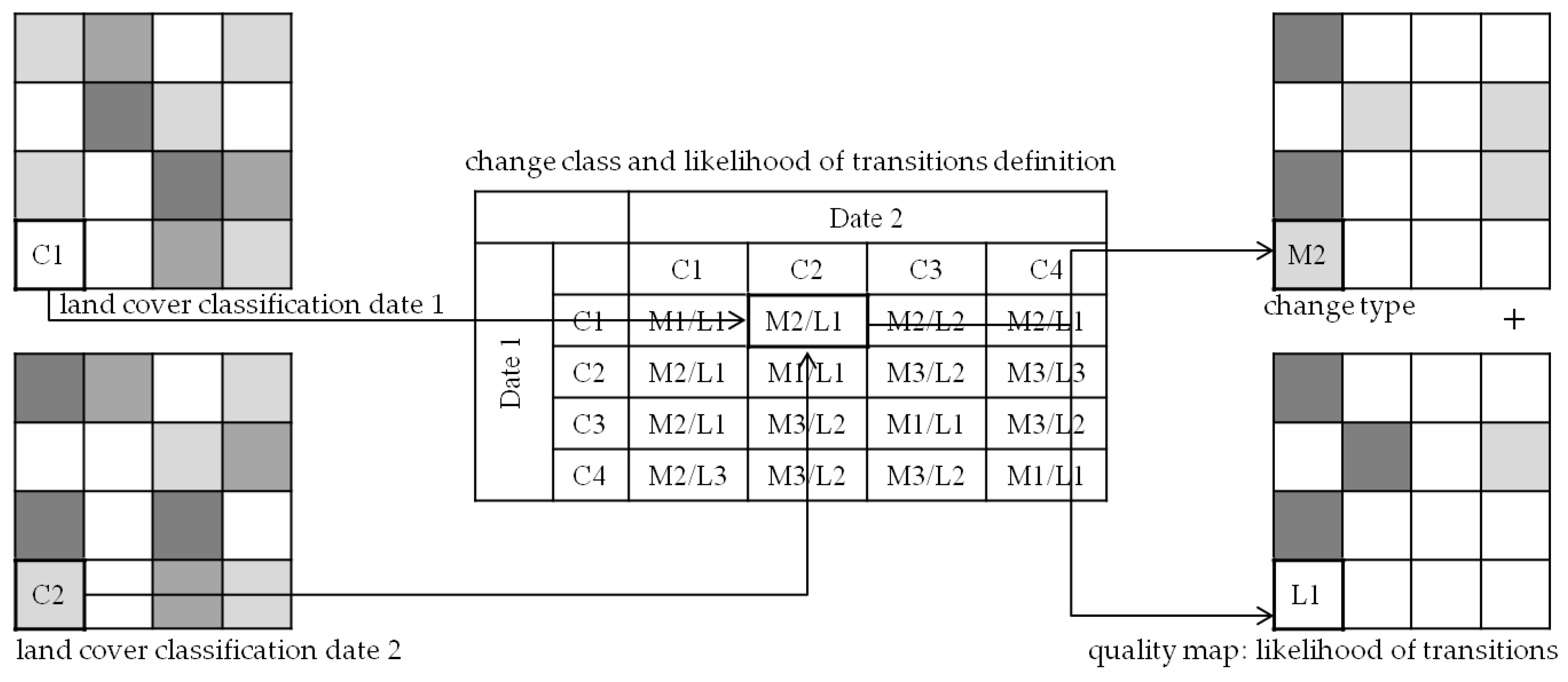
Considering one legend level and classifier, the sets of land cover classifications of the two dates were cross tabulated to obtain one set of 100 change mappings. To form the change mapping i, the attributed class of any pixel of the land cover classification i of 2008 was compared to the class of respective pixel in the classification i of 2010. This resulting transition was then reclassified considering one defined change class and the likelihood of that transition occurring, as illustrated in Figure 7.

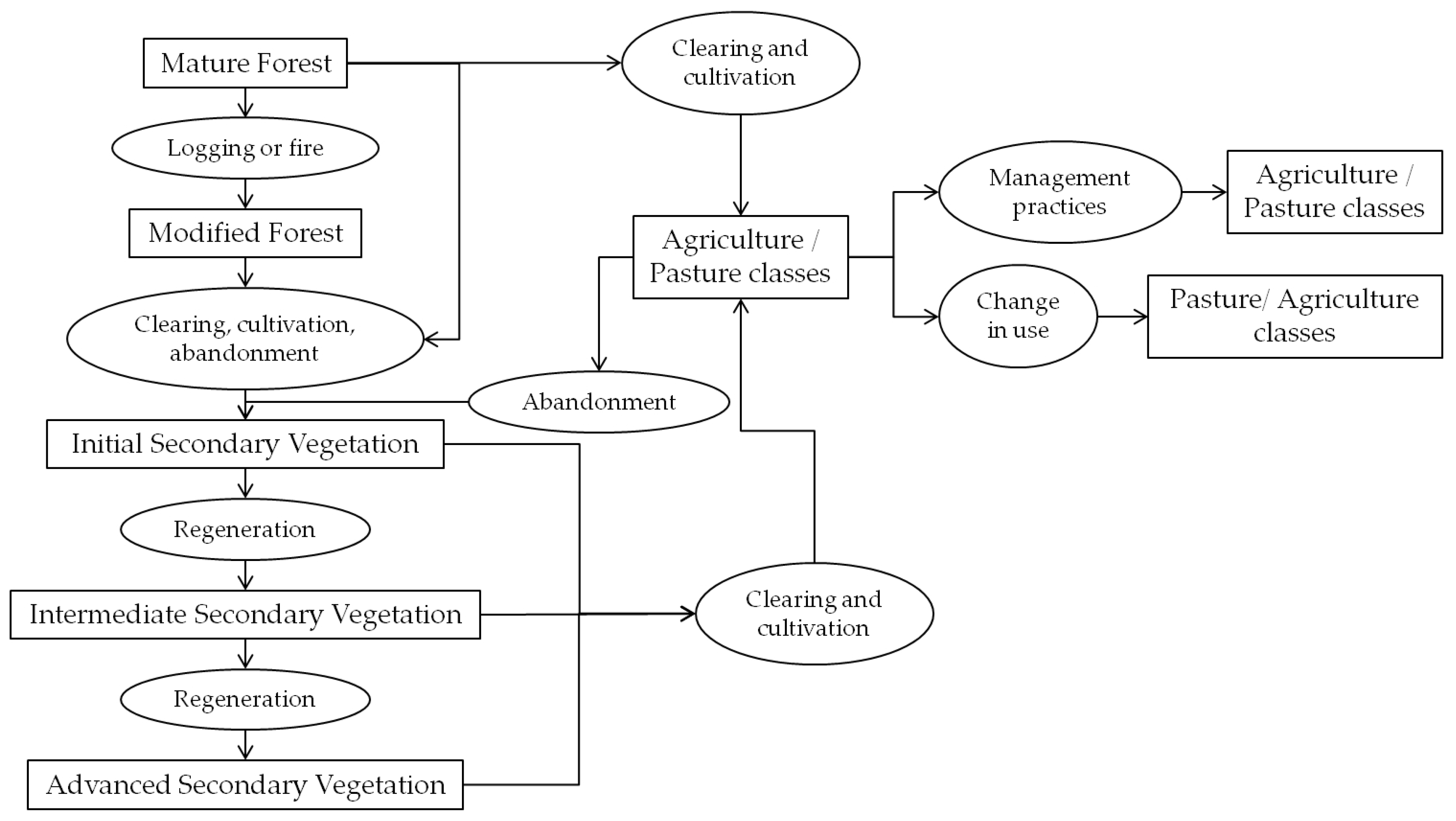
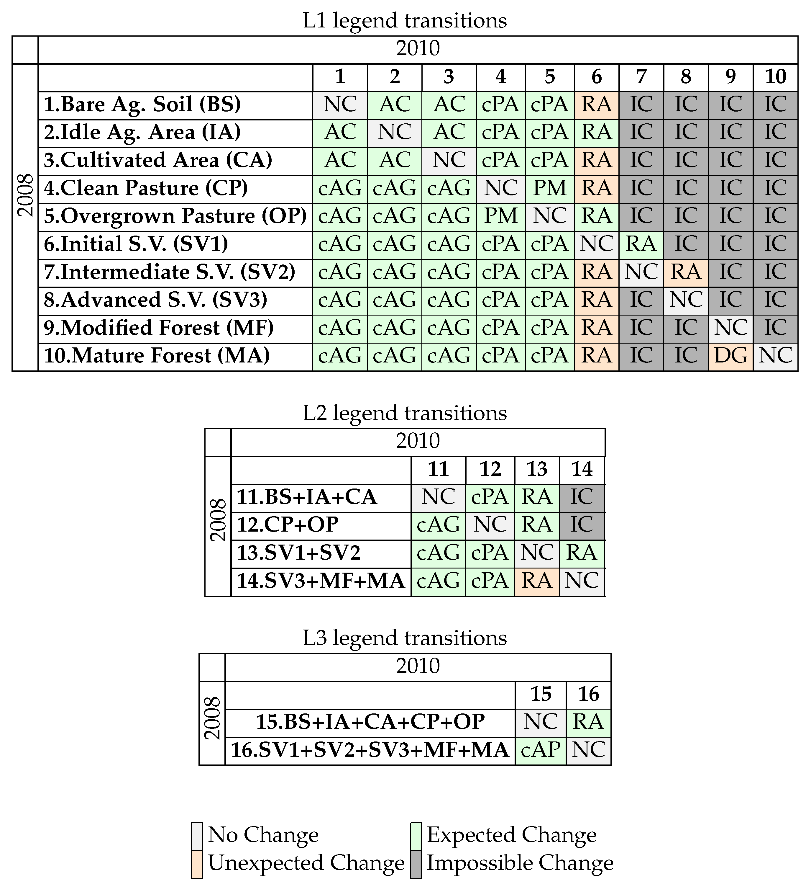
Based on the definitions of [49] and the knowledge of the studied area, the processes that results in each land cover class is illustrated in Figure 8. Change classes and likelihood of transitions were defined as follows: for each legend level, all possible combinations of land cover classes were considered for change or no change classes definition. These possible combinations (100 for L1, 16 for L2 and 4 for L3) were reclassified considering the processes necessary for these changes to occur, to form collapsed change/no change (or just collapsed change, for simplification) classes. Nine collapsed change classes were defined and are summarized in

Table 3. Collapsed change classes definition.

Acronym	Class Name	Description
NC	No Change	No change had occurred (the same class was observed in both dates)
AC	Agricultural Cycle	Changes due the annual agriculture cycle
cPA	Convertion to Pasture	Transition from one non pasture class to a pasture one
cAG	Convertion to Agriculture	Transition from one non agricultural class to an agricultural one
PM	Pasture Management	Changes due pasture management practices
cAP	Convertion to Agropasture	A forested class changing into agropasture (BS+IA+CA+CP+OP)
RA	Regeneration	Regenerating areas
DG	Degradation	Forest degradation
IC	Impossible Change	Impossible transitions, considering the two years gap

. The transitions that results in each change class are illustrated in Figure 9, along the likelihood of occurrence of each class in the field, considering the lapsed time (2 years) and the studied area. We considered four likelihood classes: No Change and Expected Change, being those considered as possible and probable transitions to occur, Unexpected Change (changes that are possible but not common) and Impossible Changes (transitions that could not happen in the field given the considered circumstances).

Transitions from any class to SV1, or a class containing SV1, were considered as Regeneration (RA). Regeneration was assigned to a change to SV1 even if the initial class was another type of forested class (SV2, SV3, MF or MA), because it is our understanding that a deforestation process has occurred in between the two year gap (2008–2010) and the area has started to regenerate. Although it is possible, regenerating right after deforestation is a very specific process, and was categorized as an Unexpected Change. Because of the time gap, transitions from BS, CA and CP to SV1 were also considered Unexpected Changes. Given the previously mismanaged state of IA and OP, transitions between these classes to SV1 were considered as Expected Changes. Transitions from SV1 to SV2 are also classified as RA and Expected Change in the studied area. A transition from SV2 to SV3, however, was considered an Unexpected Change, due to the nature of reliable reference data (since secondary vegetation classes occur into a gradient over time, the exact threshold in which an initial secondary vegetation becomes an intermediate secondary vegetation, or a intermediate secondary vegetation becomes an advanced secondary vegetation, is difficult to determine. Only areas easily identified as each secondary vegetation class were sampled. Because of the structure of sampled classes, it is believed that transitions from intermediate secondary vegetation to advanced secondary vegetation is most likely due errors in classification than real regeneration, since this change would take more than two years to occur.).

Impossible Changes encompasses mainly transitions from agropasture classes (BS, IA, CA, CP or OP) to forested classes (SV2, SV3, MF or MA) that would need more than two years to occur. The only process in which a more developed forest class would directly become less developed is Degradation (DG), which occurs only from MA to MF. Although this transition is theoretically possible considering the two years gap, MF in the studied area (within the analyzed date) is due to an understory fire that reportedly took place in the 1990s. Since a similar process was not detected in the specific time frame analyzed, this transition was considered as an Unexpected Change.

3.3. Final Change Mapping and Associate Quality Mappings

The steps for obtaining the final change mapping and associate quality mappings are illustrated in Figure 10. Each pixel in the final change mapping for each legend and classifier receives the most frequent label found in the respective pixel in the 100 mappings. If two or more labels occurred with the same frequency, the assigned label is randomly selected. Notice that classes that resulted in Impossible Changes also concurred to the post of most frequent label. As regards the cases in which this category was assigned to the final mapping, these pixels were reclassified as ‘Not Specified’ (NS). From the set of 100 mappings, two quality mappings are also calculated: the likelihood of transitions of the final change mapping and the uncertainty of the final change mapping.

The uncertainty (U) of a final change mapping was calculated by:

$$U=1-\frac{m}{n}$$

(1)

in which m is how many times the most frequent class was found and n is the total number of classifications (100 in this case). This data represents how sensitive the final change mapping is to the variation of training samples for land cover classification.

Note that along with the set of 100 change mappings, there is also a correspondent set of 100 likelihood of transitions mappings. In this study, the likelihood of the final change class mapping is given by the most computed likelihood class of transitions that resulted in the same collapsed change class of the final change mapping.

3.4. Evaluation Indexes

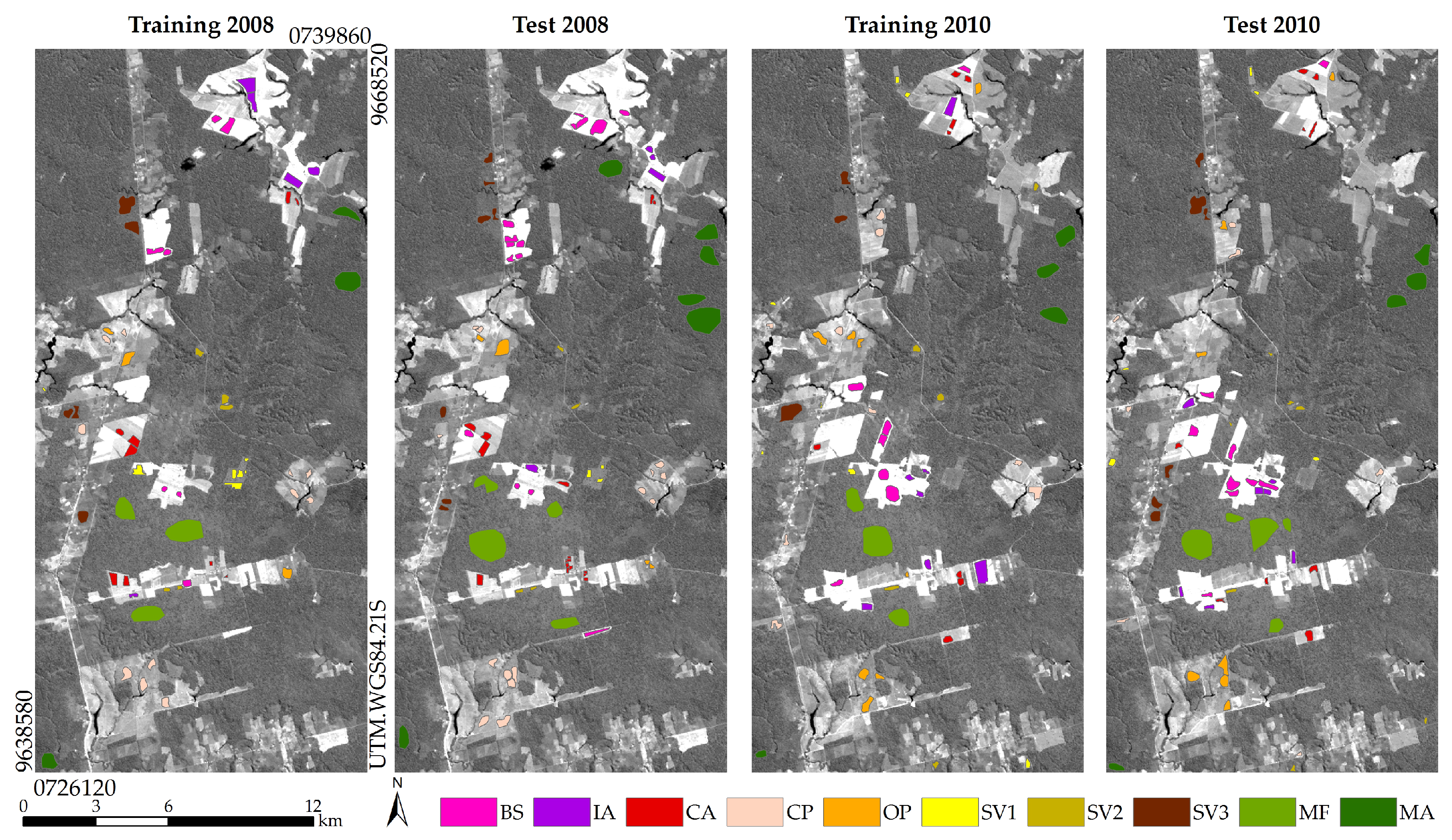
To analyze the final change mappings, samples of collapsed change classes were selected, also using PRODES, TerraClass and field data information. These samples are illustrated in Figure 11, over band 5 of TM data from 2010, for reference. The number of labeled samples is also illustrated in this figure. Note that because errors in land cover classifications may occur, impossible changes and even possible changes that didn’t occur in the field can be computed in change mappings obtained from post-classification comparison. For obvious reasons, it is not possible to find test samples for these classes, so the conventional square confusion matrix is not appropriate for this case. Likewise the solution proposed by [24], we calculated rectangular confusion matrices. These matrices were also generated using a Monte Carlo approach, in which 100 samples of each collapsed change class were randomly selected to generate one matrix. We repeated this process 10,000 times for each final change mapping. For accuracy evaluation, some suppositions were made:

• pixels/regions classified as Impossible Changes/Not Specified are areas in which we have no information and may be considered as misclassified;
• pixels/regions classified as changes from which reference samples were not found are either misclassified or are not expressive in the study, so these can also be considered as misclassified;
• reference samples are representative of respective classes in the whole classification.

Given these suppositions, it is believed that pixels/regions classified as collapsed change classes for which labeled samples were not found are clearly error areas. With the reference samples for the other collapsed change classes, it is possible to assess the accuracy of the remaining pixels/regions of the change mappings. Thus, temporally disregarding the lines in the rectangular matrix for classes from which there are not reference samples, we have a square matrix. From this square matrix, it is possible to calculate an index referred in this work as ‘Partial Accuracy’, that corresponds to the sum of the main diagonal divided by the total of samples, similar to the traditional Overall Accuracy index. Given the suppositions made, we believe that the product between the Partial Accuracy (A_p) and ‘area being evaluated’ (AE = 1 − areas supposedly misclassified/total area) is representative of the accuracy of the whole change mapping. This index will be represented as A_c:

$$A_c=A_p\times AE.$$

(2)

The suppositions made enables the evaluation of rectangular matrices. However, small changes for which we could not find referenced samples, if real, would be masked as classification errors.

For each rectangular confusion matrix from the set of 10,000 matrices (for each change mapping), we calculated one value of A_p. Following this, the value of AE of the respective final change mapping was used to calculate the values of A_c for each rectangular matrix. Note that when AE = 1 (as happened to L3 based change mappings), A_c is equal to the traditional Overall Accuracy index. The resulting mean values of A_c (one for each final change mapping) were then compared using unpaired t-test with 1% of significance level.

The two quality mappings were also used to evaluate the results, both visually and by quantitative information. To analyze the likelihood of the transitions the percentage of occurrence of each likelihood class was considered, while we used the mean value to summarize the information in the uncertainty for the final change mappings.

4. Results

Results are presented by legend level, focusing on the comparison between pixel and region based results. Some considerations about how the legend level affects the results are also made.

4.1. L1 Legend Level

The mean rectangular confusion matrices, in percentage, and evaluation indexes for final change mappings using L1 legend are presented in

Table 4. Mean rectangular confusion matrices (%) and mean evaluation indexes for final change mappings using L1 legend.

		Reference
		Pixel Based						Region Based
		NC	AC	cPA	cAG	PM	RA	NC	AC	cPA	cAG	PM	RA
Change mapping	No Change (NC)	63.5	0.7	6.2	0.0	9.8	0.0	84.5	0.8	1.2	5.1	6.3	2.0
	Agricultural Cycle (AC)	0.5	93.5	5.0	0.1	0.4	0.0	0.8	95.6	0.0	0.3	0.0	0.0
	Convertion to Pasture (cPA)	0.6	1.4	62.9	1.2	5.1	15.0	0.8	0.3	71.8	4.8	0.0	0.0
	Convertion to Agriculture (cAG)	1.4	4.5	0.0	98.7	1.0	0.0	1.1	1.7	0.0	88.9	0.0	0.0
	Pasture Management (PM)	0.3	0.0	10.0	0.0	81.4	12.3	0.0	1.6	27.0	0.0	93.7	20.6
	Regeneration (RA)	1.9	0.0	15.8	0.1	1.4	66.4	0.0	0.0	0.0	0.0	0.0	67.9
	Degradation (DG)	0.9	0.0	0.0	0.0	0.0	0.4	0.0	0.0	0.0	0.0	0.0	0.0
	Not Specified (NS)	31.0	0.0	0.1	0.0	0.8	5.9	12.7	0.0	0.0	0.8	0.0	9.5
	Accuracy of change mapping ($A_c$)	0.58 ± 0.01						0.67 ± 0.01
	Partial Accuracy ($A_p$)	0.83 ± 0.01						0.87 ± 0.01
	Area being evaluated ($AE$)	0.70						0.77

Notes: $A_c=A_p\times AE$. Both $A_p$ and $A_c$ are represented as $\mu \pm \sigma$, in which μ = mean value and σ = standard deviation of values.

. To better understand these values, the mean values for the accuracy indexes obtained by each set of 100 land cover classifications are illustrated in

Table 5. Mean accuracy values of land cover classes of L1 based land cover classifications.

Classes	2008				2010
	Pixel Based		Region Based		Pixel Based		Region Based
	PA	UA	PA	UA	PA	UA	PA	UA
Bare Ag. Soil (BS)	0.91	0.97	0.77	1.00	0.89	0.88	0.85	1.00
Idle Ag. Area (IA)	0.95	0.90	0.92	0.80	0.87	0.89	1.00	0.87
Cultivated Area (CA)	0.97	0.98	0.93	1.00	0.93	0.83	0.85	0.81
Clean Pasture (CP)	0.97	0.95	1.00	0.89	0.65	0.94	0.64	0.88
Overgrown Pasture (OP)	0.89	0.94	0.91	0.96	0.93	0.72	0.99	0.69
Initial S.V. (SV1)	0.96	0.86	1.00	0.92	0.78	0.88	0.58	0.97
Intermediate S.V. (SV2)	0.46	0.61	0.91	0.86	0.45	0.50	0.90	0.59
Advanced S.V. (SV3)	0.58	0.56	0.55	1.00	0.47	0.46	0.62	0.95
Modified Forest (MF)	0.63	0.55	1.00	0.97	0.45	0.49	0.69	0.75
Mature Forest (MA)	0.79	0.80	1.00	0.75	0.87	0.75	1.00	0.93
Overall Accuracy	0.81 ± 0.01		0.90 ± 0.02		0.73 ± 0.01		0.81 ± 0.02
Kappa index	0.79 ± 0.01		0.89 ± 0.02		0.70 ± 0.01		0.79 ± 0.02

Notes: Ag. = Agricultural; S.V. = Secondary Vegetation; PA = mean Producer Accuracy; and UA = mean User Accuracy. Overall Accuracy and Kappa index values are represented as $\mu \pm \sigma$, in which μ = mean value; and σ = standard deviation of values.

.

The mean A_c values for the two change mappings in L1 and mean accuracy indexes for land cover classification from the same year were evaluated using the unpaired t-test with 1% of significance level. Accordingly to this hypothesis test, all mean indexes values are statistically different from each other. For L1 legend, region based land cover classifications obtained a higher mean Overall Accuracy value than pixel based ones. As a result, not only a higher percentage of the area was mapped using region based classifiers (higher AE), but the mapped area is also more accurate (higher A_p), which leads to a more accurate change mapping, in general (higher A_c).

Considering the collapsed change classes, it is possible to observe that the classification of almost all classes is better in the region based change mappings, with the exception of Conversion to Agriculture. This result may be explained by the generally better classification of the agricultural classes Idle Agricultural Area and Cultivated Areas using the pixel based approach. In addition, the confusion between some pair of collapsed change classes using pixel classification seems to be minimized with region based classifications. This is the case with the pixels of (a) Conversion to Pasture being classified as either No Change or Regeneration and of (b) Regeneration being misclassified as Conversion to Pasture. However, we also observed an increment in the number of samples of Conversion to Pasture and Regeneration misclassified as Pasture Management in the region based change mapping of L1 legend, when compared to the pixel based one.

Some of the considerations made over the accuracy of the final change mappings could also be made over the likelihood of the final change mapping. The occurrence of each likelihood class (in percentage), in each final change mapping for L1 legend is presented in

Table 6. The occurrence (%) of each likelihood class in final change mappings obtained using L1 legend, calculated over the mode of change mappings.

Likelihood Class	Pixel Based Change Mapping	Region Based Change Mapping
No Change	51.3	60.6
Expected Change	17.3	16.1
Unexpected Change	2.3	1.4
Impossible Change	29.0	21.9

. As can be seen in this table, region based final change mappings obtained a lower percentage of both Unexpected and Impossible Changes. Although this result can be implied by the higher AE value of each final change mapping, it must be highlighted that previous knowledge about the changes having occurred in the pair of images being analyzed are necessary in order to obtain the AE, while the likelihood classes are calculated from the likelihood matrices presented in Table 3, i.e., considering only the studied area and time gap, and not any specific pair of images or reference samples.

In addition, Impossible Changes are, overall, due to the transition of some class to Intermediate Secondary Vegetation, Advanced Secondary Vegetation, Modified Forest or Mature Forest in L1 legend. Likewise, Unexpected Changes occur due to transitions from some class to Secondary Vegetation (SV1, SV2 and SV3) or from Mature Forest to Modified Forest in this legend. Therefore, the lower percentage value of occurrence of these classes is result of the better classification of the forested classes (classes of Secondary Vegetation, Modified Forest and Mature Forest) obtained by region based land cover classifications than by pixel based ones. The exception of this result appears to be Initial Secondary Vegetation for the 2010 land cover classifications, probably because this class occurs in small areas in the 2010 image, for which the selected segmented image may not be adequate.

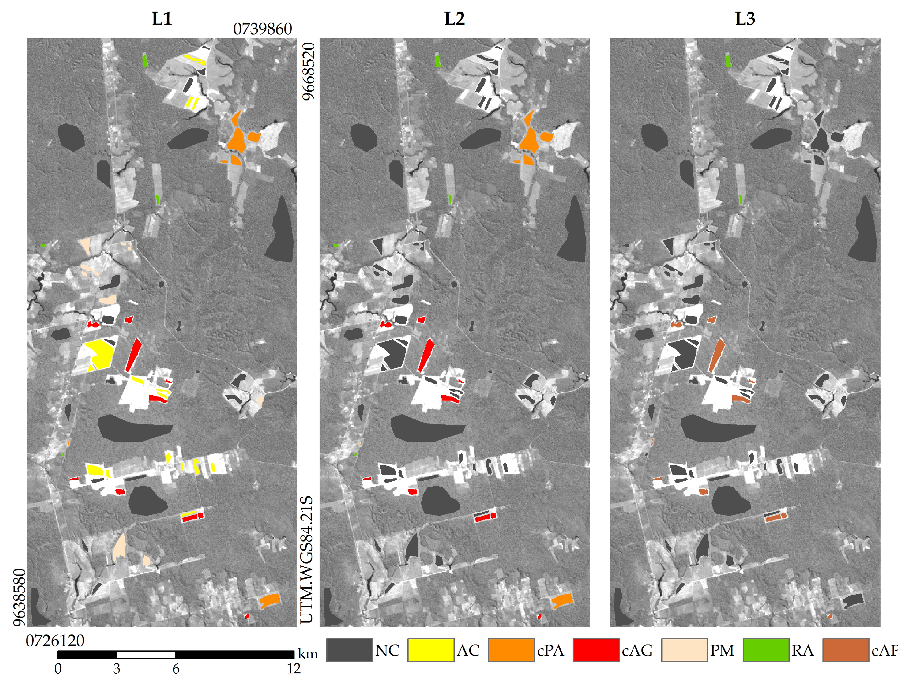
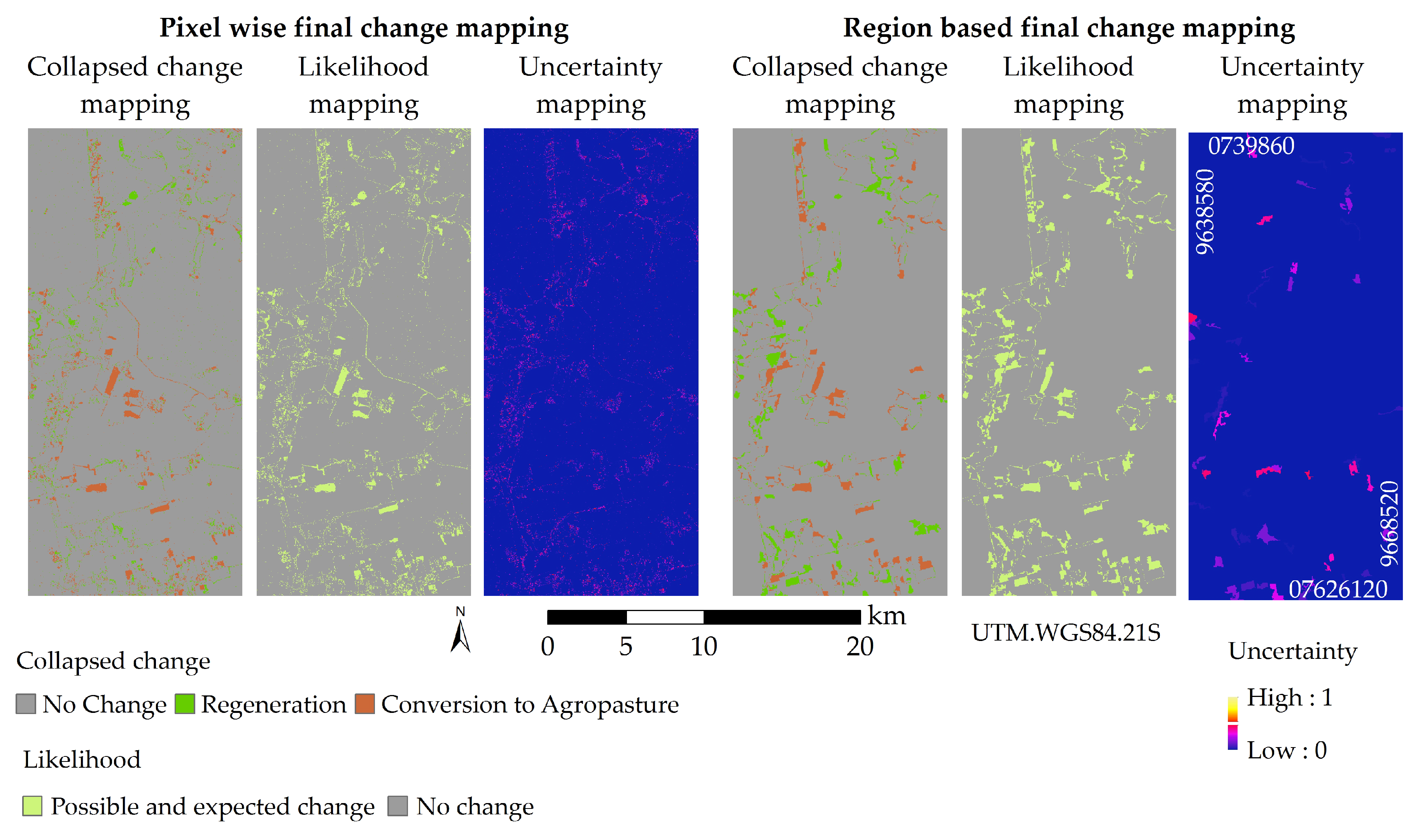
Generally, we are searching for the classification/mapping with the higher accuracy. However, it is also important that these have a low uncertainty value, since we cannot always ascertain the quality of training samples and a robust data/classifier should return stable results (even if small variations in data sampling should occur). Besides better accuracy and higher percentage of probable transitions, the final change mapping obtained with region based classification also presented a lower mean uncertainty value (5.0%) than that of the pixel one (7.0%). Furthermore, region based land cover classifications and change mappings appears to be more efficiently interpreted, since pixel based results present a scattered pattern, as illustrated in Figure 12. Here, the final change mappings for L1 legend are illustrated, as well as the respective quality mappings. As can be noted, this scattered pattern of pixel based mappings hinders the visualization and analysis of pixels that received classes from probable and expected transitions (No Change and Expected Change) among pixels that did not (Unexpected Change and Impossible Change).

4.2. L2 Legend Level

The mean rectangular confusion matrices (in percentage) and evaluation indexes for final change mappings using L2 legend are presented in

Table 7. Mean rectangular confusion matrices (%) and evaluation indexes for final change mappings using L2 legend.

		Reference
		Pixel Based				Region Based
		NC	cPA	cAG	RA	NC	cPA	cAG	RA
Change Mapping	No Change (NC)	89.0	17.0	0.3	5.9	95.7	19.6	4.9	22.5
	Conversion to Pasture (cPA)	1.3	62.5	2.0	23.7	1.0	80.4	12.7	0.0
	Conversion to Agriculture (cAG)	1.1	0.0	97.6	9.5	1.1	0.0	82.3	0.0
	Regeneration (RA)	8.4	20.5	0.1	57.7	2.1	0.0	0.1	74.7
	Not Specified (NS)	0.1	0.0	0.0	3.2	0.1	0.0	0.0	2.8
	Accuracy of change mapping (Ac)	0.77 ± 0.02				0.83 ± 0.02
	Partial Accuracy (Ap)	0.77 ± 0.02				0.84 ± 0.02
	Area being evaluated (AE)	0.99				0.99

Notes: $A_c=A_p\times AE$. Both $A_p$ and $A_c$ are represented as $\mu \pm \sigma$, in which μ = mean value and σ = standard deviation of values.

. The mean values for the accuracy indexes obtained by each set of 100 land cover classifications are illustrated in

Table 8. Mean accuracy values of land cover classes of L2 based land cover classifications.

Classes	2008				2010
	Pixel Based		Region Based		Pixel Based		Region Based
	PA	UA	PA	UA	PA	UA	PA	UA
BS+IA+CA	0.99	0.96	0.96	1.00	0.97	0.94	0.90	1.00
CP+OP	0.93	0.98	0.97	0.96	0.90	0.92	1.00	0.84
SV1+SV2	0.76	0.88	0.85	0.95	0.65	0.78	0.61	0.95
SV3+MF+MA	0.93	0.80	0.98	0.87	0.86	0.74	0.97	0.77
Overall Accuracy	0.90 ± 0.01		0.94 ± 0.02		0.84 ± 0.02		0.87 ± 0.03
Kappa index	0.87 ± 0.02		0.92 ± 0.02		0.79 ± 0.02		0.83 ± 0.04

Notes: BS = Bare Soil; IA = Idle Agricultural Area; CA = Cultivated Area; CP = Clean Pasture; OP = Overgrown Pasture; SV1=Initial Secondary Vegetation; SV2 = Intermediate Secondary Vegetation; SV3 = Advanced Secondary Vegetation; MF = Modified Forest; MA = Mature Forest; PA = mean Producer Accuracy and UA = mean User Accuracy. Overall Accuracy and Kappa index values are represented as $\mu \pm \sigma$, in which μ = mean value; and σ = standard deviation of values.

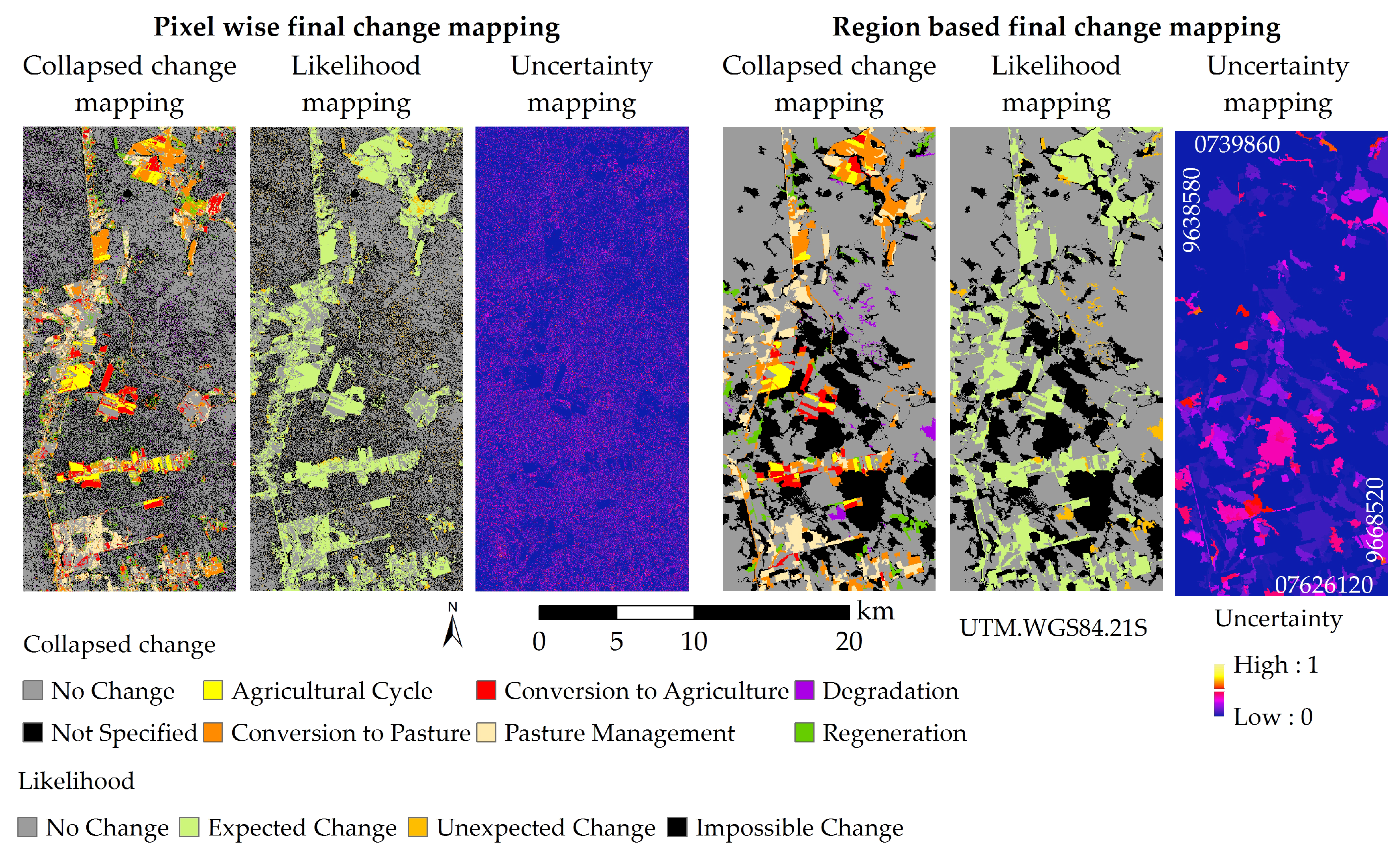
. All mean A_c values for change mappings and mean Accuracy indexes for land cover classification of the same year are statistically different considering the t-test with 1% of significance. The final change mapping and associated quality mappings for L2 legend are illustrated in Figure 13.

Similarly to the results obtained using L1 legend, we can observe that region based land cover classifications led to an overall improvement in the final change mapping when compared to the pixel based ones, with the exception of the class Conversion to Agriculture. In addition, it is possible to observe a significant confusion (higher than 20%) between the classes Regeneration and Conversion to Pasture in the pixel based final change mapping, probably due the low accuracy of the class SV1+SV2 in pixel based land cover classification. This problem, however, did not occur in the region based final change mapping, even though the class SV1+SV2 has presented a relatively low PA value in 2010 land cover classifications.

The decrease in the detail level of land cover classification from L1 to L2 led to a smaller amount of impossible transitions. The transitions that lead to Unexpected Changes and Impossible Changes, in L1, sums 42.0% of the transitions between land cover classes. In L2, this number decreases to 18.8%. The smaller probability to obtain an Unexpected or Impossible Change, allied to the higher accuracy of land cover classifications, results in the lower percentage of these likelihood classes in L2, as illustrated in

Table 9. The occurrence (%) of each likelihood class in each final change mapping obtained using L2 legend.

Likelihood Class	Pixel Based Change Mapping	Region Based Change Mapping
No Change	82.0	84.5
Expected Change	12.7	11.8
Unexpected Change	4.8	2.3
Impossible Change	0.5	1.4

, and obviously in the higher percentage of AE in L2 final change mappings. In addition, the mean uncertainty of the final change mapping also presented low values (3.7% for pixel based and 1.7% to region based final change mappings).

4.3. L3 Legend Level

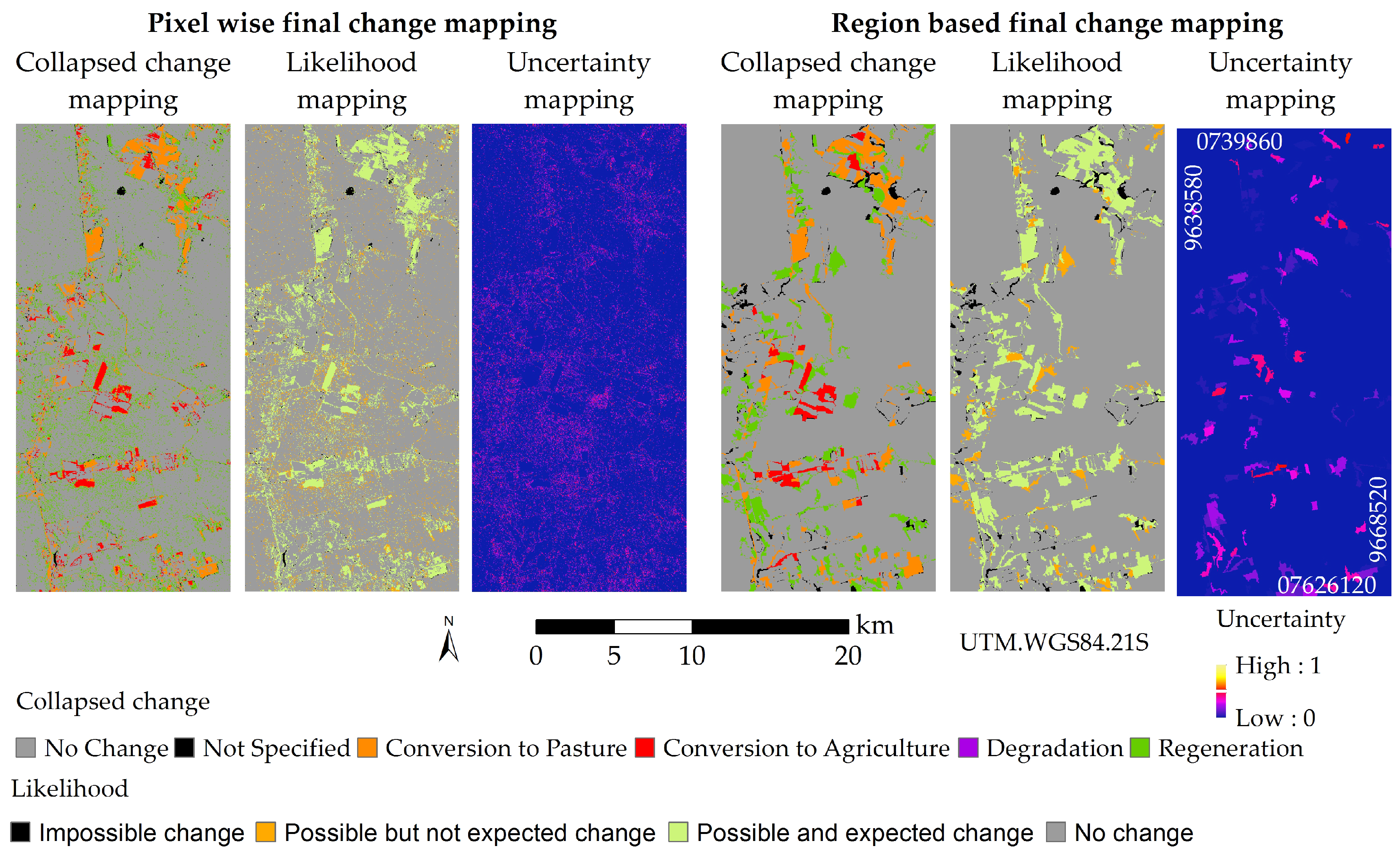
The final change mapping and associated quality mappings for L3 legend are presented in Figure 14. These mappings present some characteristics that differentiate between the ones obtained in L1 and L2 legend. Due to the reduction in legend detail, only three collapsed change classes are possible in L3 legend: No Change, Regeneration and Conversion to Agropasture. These three classes are considered as possible and probable. Furthermore, reference samples were found for all collapse change classes. Therefore, the likelihood of the final change mapping becomes a binary change and no change map, that is easily derived from the final change mapping itself. It also means that the confusion matrices for the change mappings of this legend level are square, so the A_c index becomes the traditional Overall Accuracy index. In addition, the analysis of uncertainty also leads to small gain in information, since both have a mean uncertainty value lower than 1%.

The square mean confusion matrices for L3 legend final change mappings are illustrated in

Table 10. Mean rectangular confusion matrices (%) and evaluation indexes for final change mappings using L3 legend.

		Reference
		Pixel Based			Region Based
		NC	RA	cAP	NC	RA	cAP
	No Change (NC)	98.9	39.7	9.2	99.6	27.8	12.5
Change mapping	Regeneration (RA)	0.7	59.8	0.0	0.3	72.2	0.0
	Conversion to Agropasture (cAP)	0.4	0.5	90.8	0.1	0.0	87.5
	Overall Accuracy	0.83 ± 0.02			0.86 ± 0.02

Note: Overall Accuracy is represented as $\mu \pm \sigma$, in which μ = mean value and σ = standard deviation of values.

, along with the mean Overall Accuracy index. The accuracy indexes of the sets of land cover classification are presented in

Table 11. Mean accuracy values of land cover classes of L3 based land cover classifications.

Classes	2008				2010
	Pixel Based		Region Based		Pixel Based		Region Based
	PA	UA	PA	UA	PA	UA	PA	UA
BS+IA+CA+CP+OP	0.99	0.99	1.00	1.00	0.99	0.98	0.93	0.99
SV1+SV2+SV3+MF+MA	0.99	0.99	1.00	1.00	0.98	0.99	0.99	0.94
Overall Accuracy	0.99 ± 0.01		0.99 ± 0.01		0.99 ± 0.01		0.96 ± 0.02
Kappa index	0.99 ± 0.01		0.99 ± 0.01		0.98 ± 0.01		0.92 ± 0.04

Notes: BS = Bare Soil; IA = Idle Agricultural Area; CA = Cultivated Area; CP = Clean Pasture; OP = Overgrown Pasture; SV1 = Initial Secondary Vegetation; SV2 = Intermediate Secondary Vegetation; SV3 = Advanced Secondary Vegetation; MF = Modified Forest, MA = Mature Forest; PA = mean Producer Accuracy; and UA = mean User Accuracy. Overall Accuracy and Kappa index values are represented as $\mu \pm \sigma$, in which μ = mean value; and σ = standard deviation of values.

. Mean Overall Accuracy for final change mappings and mean accuracy indexes for land cover classifications of the same year were statistically different from each other considering unpaired t-test with 1% of significance level, although some truncated values are the same in Table 11. As can be seen, although region based classification led to a slightly more accurate final change mapping, it is possible to perceive that the change class Conversion to Agropasture were better classified using pixel based land cover classifications. This probably happened because of the lower accuracy of the classification of the agropasture class (BS+IA+CA+CP+OP) in the region based land cover classifications of 2010.

5. Discussion

Three legend levels were considered in this study, with different levels of detail. For all legend levels, change mappings obtained from region based classifications were more accurate, presented a lower percentage for areas in which impossible or unexpected changes occurred and presented a lower mean uncertainty value. For the two legends with higher detail level, we observed a general improvement in all change classes while using the region based approach, with the exception of Conversion to Agriculture. The same behavior was observed in the legend with the lower number of classes, with the corresponding class Conversion to Agropasture. This result is explained by slightly better classification of some agricultural classes using the pixel approach. Another peculiarity is that classes occurring in small features, such as Initial Secondary Vegetation in the 2010 image, are better classified using the pixel based Maximum Likelihood classifier. It happens because these features were not adequately represented in the segmented image used, since all segments had at least 100 pixels. In this sense, it may be interesting to consider a multi scale approach, in which different segmented images are selected to classify each land cover class.

Considering the different legend levels presented, the reduction of detail level in both land cover and land change legends led to higher accuracy values and decreased the occurrence of Impossible Changes and resulting Not Specified areas. However, as discussed before, the proposed quality mappings (likelihood and uncertainty) seems to be less useful as the legend becomes more generalized (fewer classes). It is also probable that the number of impossible or improbable transitions would decrease if a larger time span was evaluated, further hindering the analysis. As mentioned by [41], the likelihood matrices are strongly dependent on the time interval considered and the environmental context. In this work, not only empiric and theoretical knowledge of the ecological succession characteristics of the studied area were needed, but also specific knowledge about the management of pasture and agricultural classes in the area. Further knowledge of the agents of forest degradation in the specific time being considered is also necessary. Although part of our proposed likelihood matrix can be generalized for the Brazilian Amazon, it must be highlighted that its construction is a delicate and complex process. The usage of the proposed methodology in another area, with different land cover classes and time interval, would require the construction of adequate likelihood matrices, which may demand expert knowledge.

Specially regarding L3 legend level in this work, despite the very high mean accuracy indexes values for land cover classifications, the final change mappings presented an Overall Accuracy lower than 90%. Although these values may be considered high, it must be highlighted that changes usually occur on a scale lower than 10% in tropical forests and within small time gaps, mainly when considering such a small amount of land cover or change classes. It means that even with accurate land cover classifications, it is possible that the resulting change mapping will not be accurate enough to be useful for the monitoring of a given area. In the case of the studied area, we can observe that the least accurate change class was Regeneration, for both classification approaches. Since samples of this class were found in few and small features, mainly for L3 legend, tests using similar data in which we have more samples of Regeneration are needed to verify the usefulness of this legend level.

Uncertainty analysis does not present clear accuracy related characteristics, but it may be important to help the analyst to identify problems in either the data used or in the land cover classification/change mapping. For example, the presence of high uncertainty areas either means high presence of mixed pixels or non spectral separability of the chosen classes, which means the data used may not be suitable for the study, or that the training set is not representative of the classes.

As cited in many change detection studies, the use of post-classification comparison for detecting changes has one clear drawback: errors in individual classifications leads to false positive or false negative changes. As observed in this study, the accuracy of the change mappings may not be high enough for operational purposes, in any legend level or considered generalization. Likewise what was observed in [24], the results presented in this study show that the use of this change detection technique not only leads to the detection of changes in static areas or the no detection of real changes, but some detected changes are due to absurd transitions. Changes resulted from such transitions are clearly errors in classification and need to be highlighted. Change detection works based on post-classification comparison, mainly those with detailed legends, should consider both uncertainty related measures as well as the likelihood of transitions for evaluating results, even if the usefulness of the proposed quality mappings seems to decrease along the detail of the legend. Actually, either analysis may be useful to improve not only change detection, but land cover classification as well. Moreover, the existence of impossible changes expose clear errors in one or both land cover classifications, facilitating the process of analysis and correction. We also observed a high amount of samples of No Change in which Impossible Changes were detected, when using the most detailed legend level. This happened mainly in areas pertaining to forest classes in both dates that were misclassified, for some reason, as secondary vegetation. Since binary methods has presented high accuracy for change/no-change mappings [50] it is expected that firstly separating these two classes and then classifying the changes (use of a hybrid change detection methodology) can improve the results.

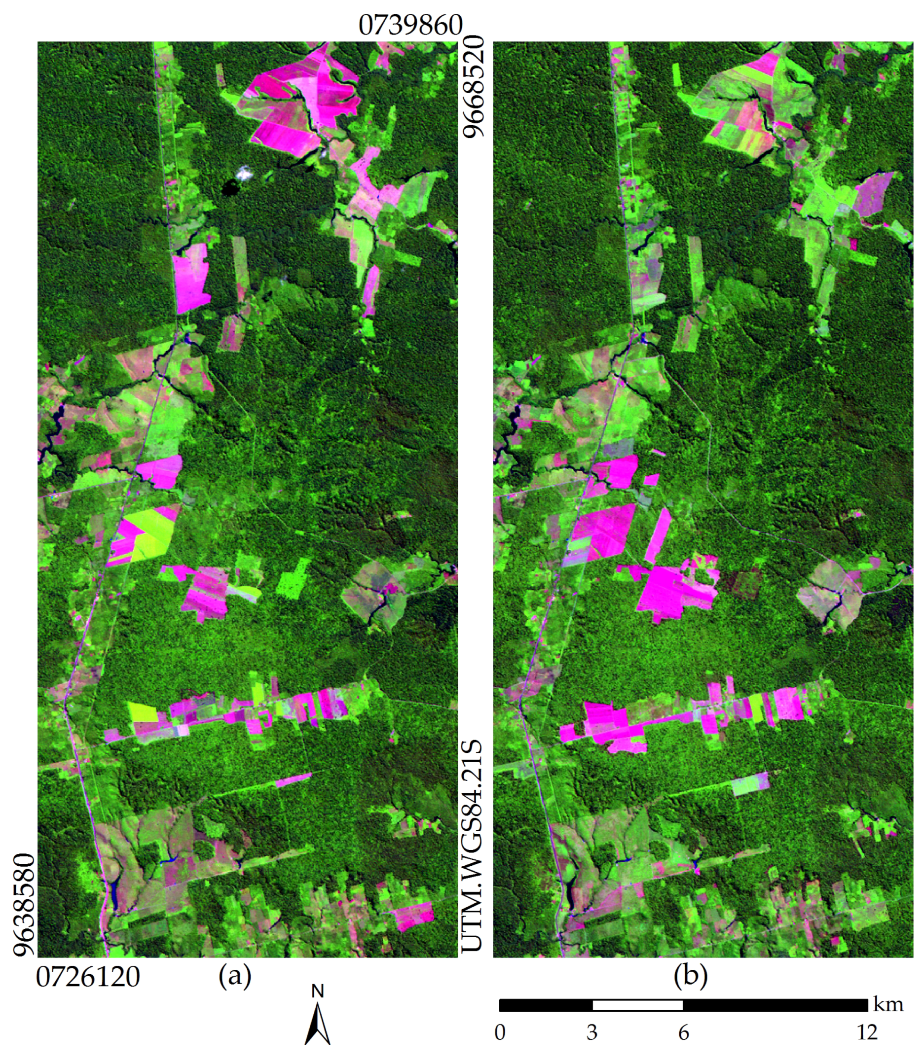
6. Conclusions

This work aimed to present a multi-legend change detection study, comparing change mapping obtained by post-classification comparison of land cover classifications generated by pixel and region based classifiers. These change mappings are derived from a set of other 100 change mappings, obtained from sets of 100 land cover classifications of a LANDSAT5/TM image from two dates, namely June of 2008 and 2010. Two quality mappings associated to the change mappings were also proposed: one based on the uncertainty of the respective change mapping and one based on the likelihood of transitions that resulted in the change mapping. This second quality mapping has the potential to improve post-classification comparison results by the indication of areas in which impossible or unexpected changes were mapped, which are problems often neglected in usual post-classification comparison studies. For the most detailed legend (L1) and considering the likelihood of transitions, it was possible to identify that at least 29.0% of the pixel based change mapping and 21.9% of the region based change mapping are misclassified, with no need of reference data. Thereby, analyzing the theoretical possibility of transitions revealed to be a useful way to evaluate results, mainly if no reference samples can be found. It is also useful to further understand both the pattern of changes being mapped and persistent errors present in land cover classifications, which can be masked in unsuitable reference samples or just not evaluable in multi-temporal analysis due to inherent assessment difficulties. However, the usefulness of the likelihood of transitions seems to decrease along the level of detail (number of classes) in the legend.

Regarding pixel or region based classifications approaches, the results presented in this study showed that the use of region based approaches led to increased global accuracy of the change mappings, respectively of 15.5%, 7.8% and 3.6% for mappings using the legends with the higher, intermediate and lower level of detail. Thereby, the more detailed the legend, more significant the use of region based classification appears to be. In addition, individual transitions between land cover classes were better identified using the region based approach, with the exception of transitions from a non agriculture class to an agricultural one.

The decrease in detail level of the legend (the number of classes) in the land cover classifications led an increase in accuracy, which induced an apparent increase in the accuracy of the resulting change mappings. Regardless of this result, it was observed that even change mappings obtained from very accurate land cover classifications (Overall Accuracy higher than 0.98) can present accuracies not high enough for operational purposes (Overall Accuracy around 0.83).

We opted to explore the use of low processed LANDSAT5/TM data in this work, in both region and a pixel based simple approaches. Future works should consider both the use of texture measures to improve land cover classification, as well as changes in shape, boundary, homogeneity or topological information [36,51]. The use of multi-sensor data may be unavoidable in change detection studies in tropical areas, where constant cloud cover limits the acquisition of suitable optical data. In this context, similar studies using Synthetic Aperture Radar (SAR) data are necessary, mainly because change detection studies involving this kind of data has been generally focused on the comparison and creation of new binary (change/no change) change detections techniques [52,53,54,55,56,57]. Future works should consider the use of SAR data in mono and multi-sensor change detection studies, as well as hybrid change detection approaches, such as the combination of binary and post-classification methods, for accuracy improvement. The proposed methodology should also be tested considering larger time periods, with good results expected when considering more than two analyzed dates, and in larger study areas to cover some types of changes that did not occur in the area and time analyzed in this work.