Technical Note

An Improved Estimation of Regional Fractional Woody/Herbaceous Cover Using Combined Satellite Data and High-Quality Training Samples

1
College of Urban and Environmental Sciences and MOE Laboratory for Earth Surface Processes, Peking University, Beijing 100871, China
2
College of Resources Science and Technology, Beijing Normal University, Beijing 100875, China
3
Institute of Surface-Earth System Science, Tianjin University, Tianjin 300072, China
*
Author to whom correspondence should be addressed.
Remote Sens. 2017, 9(1), 32; https://doi.org/10.3390/rs9010032
Submission received: 25 October 2016 / Revised: 20 December 2016 / Accepted: 28 December 2016 / Published: 2 January 2017

Abstract

:
Mapping vegetation cover is critical for understanding and monitoring ecosystem functions in semi-arid biomes. As existing estimates tend to underestimate the woody cover in areas with dry deciduous shrubland and woodland, we present an approach to improve the regional estimation of woody and herbaceous fractional cover in the East Asia steppe. This developed approach uses Random Forest models by combining multiple remote sensing data—training samples derived from high-resolution image in a tailored spatial sampling and model inputs composed of specific metrics from MODIS sensor and ancillary variables including topographic, bioclimatic, and land surface information. We emphasize that effective spatial sampling, high-quality classification, and adequate geospatial information are important prerequisites of establishing appropriate model inputs and achieving high-quality training samples. This study suggests that the optimal models improve estimation accuracy (NMSE 0.47 for woody and 0.64 for herbaceous plants) and show a consistent agreement with field observations. Compared with existing woody estimate product, the proposed woody cover estimation can delineate regions with subshrubs and shrubs, showing an improved capability of capturing spatialized detail of vegetation signals. This approach can be applicable over sizable semi-arid areas such as temperate steppes, savannas, and prairies.

Graphical Abstract

1. Introduction

Vegetation cover information is fundamental for delineating plant distribution and understanding vegetation dynamic at local, regional, and global scales [1,2,3]. As the coexistence and conversions of woody and herbaceous covers dominate most semi-arid areas, such as the East Asian steppes, African savannas, and American plains [4,5,6], mapping fractional woody and herbaceous cover become a priority topic with relevance to ecosystem function research including regional carbon modeling, ecological assessment, and resources monitoring [7,8,9].
Remote sensing is regarded as the most feasible method and provides a key source of data for mapping vegetation cover [10,11,12,13,14]. Satellite products, such as composites and multi-temporal metrics from the Moderate-Resolution Imaging Spectroradiometer (MODIS) sensor become more and more capable of performing land surface characterizations at large scale. A global dataset named MODIS Vegetation Continuous Field (MODIS-VCF, MOD44B; 17), which is based on a regression tree model using satellite images as training samples and phenological metrics as model inputs, gives a continuous estimation of tree cover at MODIS-pixel resolution across the world. However, this product shows significant uncertainty in semi-arid areas with low tree density (i.e., wooded grasslands and sandy lands) [15]. Since semi-arid regions usually consist of various closed and open communities with a wide variation of species component, physical structure, chemical composition, and phenological phase [16], features of these vegetation canopies vary intensively. The reduced authenticity of estimation may be mainly caused by inadequate model inputs and unreliable training data, resulting in a limitation of capturing spatial detail of vegetation covers [17,18]. Hence, two efforts must be made to provide improved regional estimations of woody and herbaceous vegetation covers across semi-arid areas by using appropriate model inputs and high-quality training samples.
Multiple satellite data are considered to be used as model inputs. A suite of MODIS-derived data including specific composites (e.g., annual maximum Normalized Difference vegetation Index NDVI) and some temporal metrics (e.g., the range of NDVI during the growing season) are preferred as model inputs for mapping vegetation fractional cover [19,20]. They represent an advance in describing vegetation cover due to their capability of depicting phenology for different vegetation cover types. However, the various levels of processing change the spatial fidelity of the input data. Mapping fractional woody and herbaceous vegetation cover only using these MODIS data may result in a significant loss of vegetation cover heterogeneity [21]. Thus, other satellite observations that are sensitively associated with spatial characterizations of vegetation covers can be considered as auxiliary data to improve the capability of capturing vegetation signal during mapping procedures. For example, bioclimatic and topographic conditions usually influence the vegetation distributions [22]; land cover may also be useful since it provides information on vegetation phenology [23,24]. Since combining multiple data as inputs can introduce noise, as well as reduce spatial fidelity, estimation models should be generated with different predictor variable sets as experiments to find the most appropriate inputs for mapping fractional woody and herbaceous vegetation cover, respectively.
Quality-training samples for estimation are considered, generated from high-resolution images. In semi-arid areas, woody and herbaceous vegetation usually exhibits a high level of coexistence and conversion with many formations (e.g., tree, shrub, subshrub, herb, and bunchgrass). As the limited spatial detail of moderate remote sensing misses the small-scale woody and herbaceous vegetation variability [25], the training data could be achieved using high-resolution satellite data from the generation of images with meter or sub-meter sampling distances (e.g., IKONOS, QuickBird). Most importantly, as excess variation of inappropriate sample information causes strong indeterminacy for model results in study region with high vegetation cover heterogeneity; thus, spatial sampling should be designed to improve the levels of sample representativeness. Hence, we need to collect high-resolution highly-representative images along a spatial sampling layout formed by an efficient sampling strategy.
With the aim of producing improved regional maps of fractional woody and herbaceous vegetation covers that span the East Asia steppe, an approach was developed in this study using multiple remote sensing datasets as predictor inputs and high-quality reference data derived from high-resolution images as training samples. The tree-based regression model Random Forest was used to relate satellite predictor variables with corresponding training samples. In this study measures were implemented to expectantly improve estimation performance and accuracy spanning large semi-arid areas, involving a standardized pre-processing to establish uniform multiple inputs and an efficient spatial sampling used to collect representative training samples. Comparing with other methods, the proposed approach emphasizes:
  • Multiple satellite data combined and used as RF model inputs for estimation; and
  • High-quality training samples of representative based on a spatial sampling layout formed by a tailored sampling strategy.

2. Materials and Methods
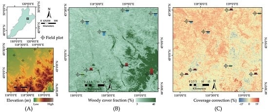
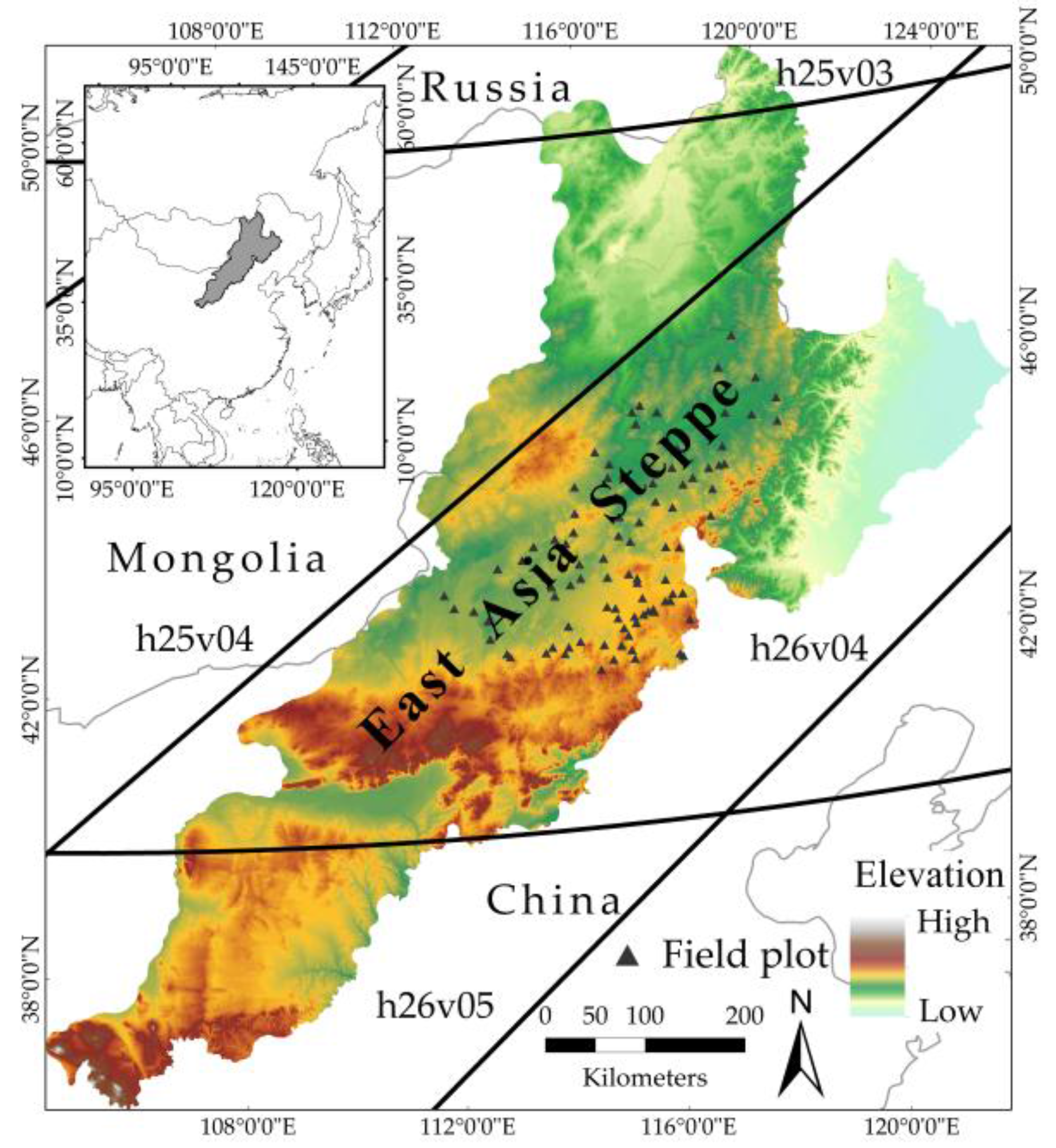
2.1. The Study Area

The East Asia steppe (covering between roughly 36°7′N–50°48′N and 104°18′E–124°21′E), which spans Northern China, Eastern Mongolia, and Southern Siberia of Russia (Figure 1), is dominated by semi-arid grasslands with embedded forest and scrub patches [26]. It has a total area of approximately 805,000 km2 with complex geomorphic types (e.g., treeless flatlands, gently rolling hills, wetlands, and mountains). This eco-region has a temperate continental climate with cold, dry winters, and warm summers and, in particular, mean annual precipitation (MAP) has an obvious gradient, ranging from 250 to 450 mm under the slight influence of the East Asian monsoon. Due to the variability of climate, topography, and soil conditions, this region shows a gradual decrease of woody cover from the southeast to the northwest and a mosaic of woody and herbaceous vegetation in the main part of the study region.
Much of the study area has experienced a rapid population and economic growth over the last 30 years, which has had a significant impact on land surface characteristics [27]. Although agricultural expansion, overgrazing, and growing demand for fuel wood have caused widespread ecosystem degeneration [28], conversion of cropland to grassland or forest has accelerated due to a series of ecological restoration policies [29]. As a consequence of its large extent and complex nature-human interactions, this region is characterized by an extensive mixture of vegetation mosaics and complex transitions from closed to open vegetation.

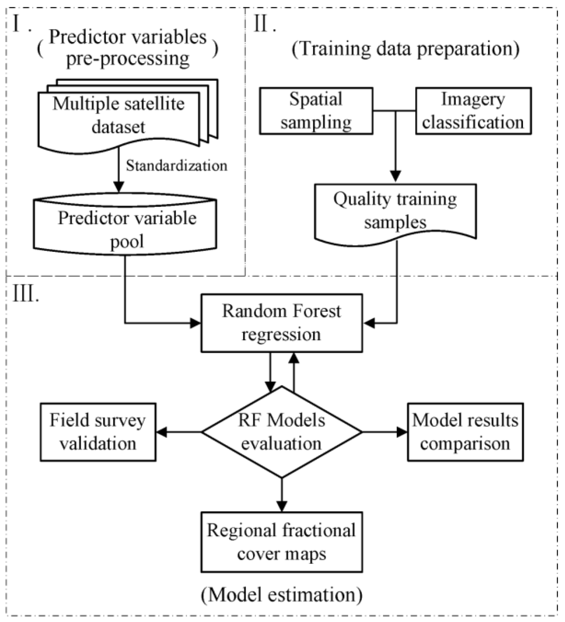
2.2. Data Handling and Methods

The process on producing regional maps of fractional woody and herbaceous vegetation cover spanning the East Asia steppe is briefly presented in Figure 2. Three main parts of work were implemented during the whole analysis:
  • A suite of statistics and metrics of satellite data from multiple sources were pre-processed into a uniform format as the predictor variable pool;
  • Training data were prepared using a sampling strategy and a human-machine interactive classification method; and
  • RF models were developed with different predictor sets to find out the most appropriate combination of predictor inputs.
By comparing different model results and validating with field measurements, the optimized estimates were kept as regional maps of vegetation fractional covers.

2.2.1. Predictor Data Pre-processing

Spectral variables were extracted from a MODIS standard product (MOD13Q1, Collection 5). In this study we focused on four MODIS tiles (H25V03, H25V04, H26V04, and H26V05). The mean, minimum, maximum, amplitude, and standard deviation of the vegetation and reflectance indices within the growing season were calculated. Additionally, ancillary data on biological climate condition, topographic information, soil type, and land-cover information were assembled. The information of all types of predictor variables is shown in Table 1.
After a series of pre-processing steps including missing data interpolation through weighted average or k-Nearest Neighbor, re-projection to equal area projection, re-sampling, and normalization, the original satellite data were converted into a multiple-band grid cell dataset. This dataset was used as predictor variable pool for establishing estimation models.

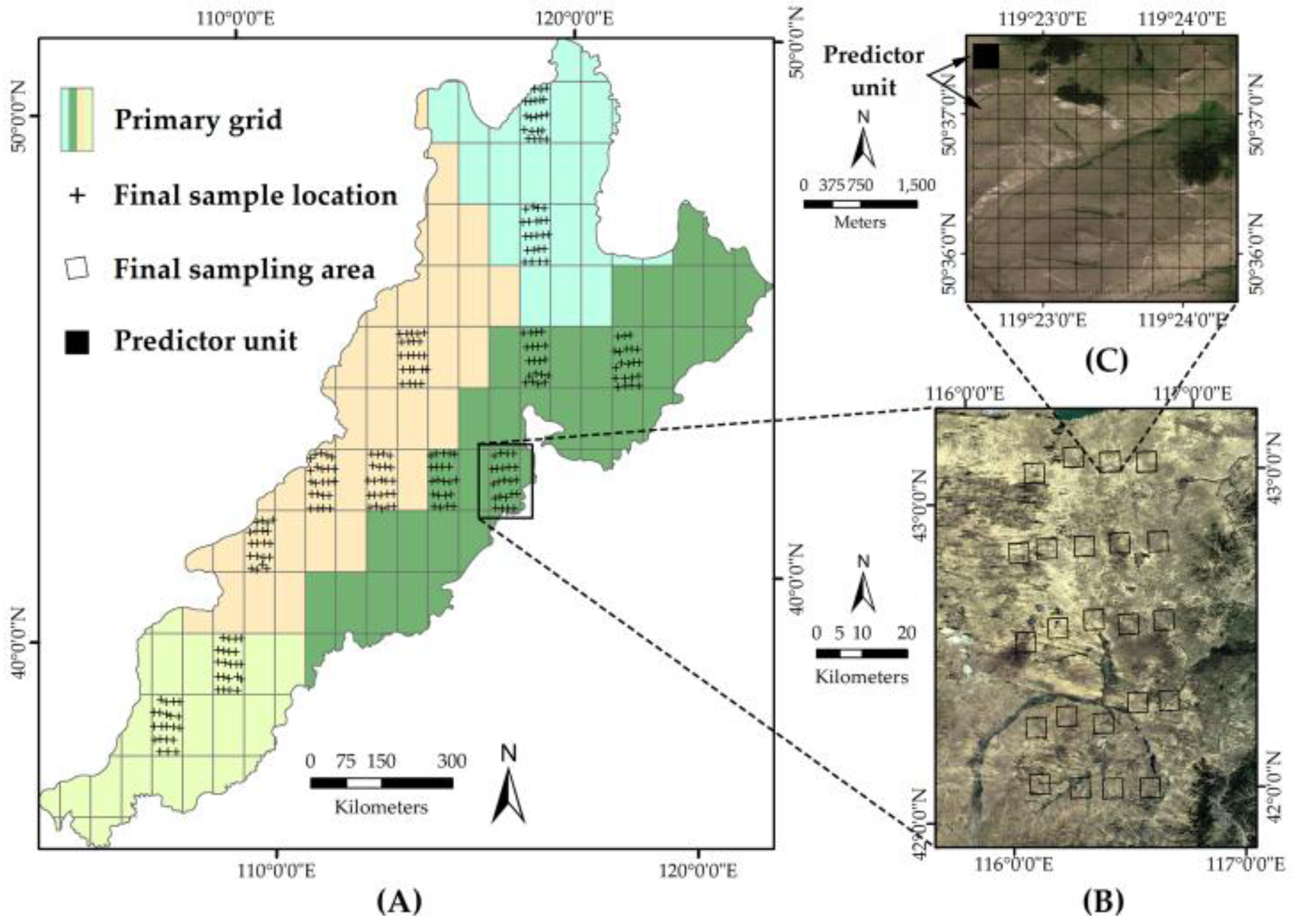
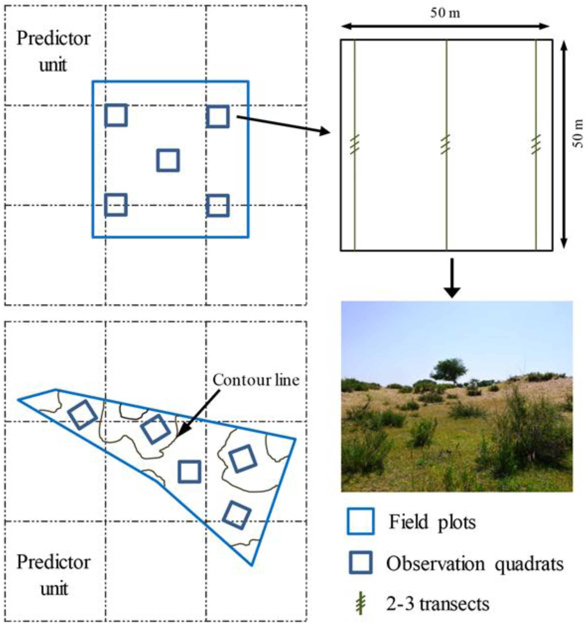
2.2.2. Training Data Preparation

We implemented a two-step spatial sampling to form a spatial sampling layout to collect highly representative samples at an appropriate sample size. The spatial sampling strategy consisted of the following two steps (Figure 3).
  • We first divided the whole study area into four independent zones by its patterns of environmental features and land-use intensity (domain knowledge); and
  • After division, a two-phase sampling was used to form a spatial sampling layout to determine final sample locations. That is, simple random sampling (SRS) was used to select primary grids in each zone. Then final sample locations were confirmed using systematic sampling (SYS) in each primary grid.
High-resolution images with preset sampling coordinates were collected from Google Earth to derive vegetation cover information. The specific advantages of using Google Earth image for reference data have been explained in Clark et al. The images were then classified into discrete classes using a human-machine interactive classification method. Within each sample two interpreters estimated the percentage cover of six ground cover types including woody vegetation and herbaceous vegetation by tailored criteria for identification. Classification results from the two interpreters were then compared and selected by expert.

2.3. Building Random Forests

Eight different predictor variable sets were assembled to generate Random Forest models respectively: (1) Specific metrics of vegetation indices (i.e., NDVI, EVI) and reflectance indices (i.e., Blue, Red, NIR, and MIR); (2) Set 1 + land-cover and soil type; (3) Set 1 + Bioclimatic variables; (4) Set 1 + topographic variables (Elevation, Slope, Aspect); (5) Set 2 + Bioclimatic variables; (6) Set 2 + topographic variables; (7) Set 3 + topographic variables; and (8) all variables. For this analysis, optimizing inputs for mapping was mainly based on the assessment of model performance, which was expressed as modeling bias and normalized mean square error (NMSE) in this study. NMSE was calculated as:
NMSE = i = 1 n ( y i y ^ i ) 2 i = 1 n ( y i y ¯ i ) 2
where y ^ i denotes the predicted value for the i-th sample, y i denotes the observed value for the i-th sample, and y ¯ i represents the mean of all observations. In this equation, a smaller score suggests better predictive capability. Hence, the RF models with appropriate predictor sets at lowest biases and NMSEs were selected for mapping fractional woody and herbaceous vegetation covers in the East Asia steppe, respectively. In order to find how each type of predictor variables rank in chosen models in terms of variable importance, we calculated variable importance indicated by a measure called the increase in mean squared error (%IncMSE) for each predictor variable. These importance scores were then accumulated for each variable type.

2.4. Field Validation

The remote sensing based estimations were validated with field data collected in July and August 2012. Cover fractions were surveyed on 110 plots located in the central part of the East Asia steppe (Figure 1). The investigation at each plot was implemented using a five-quadrant sampling mode, where the mean percent woody and herbaceous covers were calculated for each field plot from the records of five quadrats. These average values were then compared with the mean satellite estimates of a matrix consisting of nine predictor units covering the plot places (Figure 4).

3. Results

3.1. Experiments with Predictor Variables

As shown in Table 2, although RF models had relatively similar deviations (absolute value), they still achieved slightly different NMSEs. Along the addition of auxiliary satellite data, these models showed a steady increase in model performance, with the results on estimating woody plants generally exceeding that of estimating herbaceous vegetation when the models shared the same inputs. Models for woody vegetation estimation using only spectral metric variables (Set 1) resulted in non-determinacy, with a NMSE of 56%. Combining multiple satellite variables (Set 8) decreased the NMSE by 9.1%. Similarly, when spectral information was integrated with biological climate variables and land-cover information (Set 5), the NMSE of the herbaceous vegetation model decreased by approximately 13%. Hence RF models with Sets 8 and 5 were implemented for mapping percent woody and herbaceous vegetation cover in East Asia steppe respectively.
According to the variable components of selected RF models, the summed scores of variable importance in each variable type were listed in Table 3. For both woody and herbaceous vegetation, optical reflection variables, greenness indices, and biological climate variables provided main contributions to model estimation, which suggested that the integration of predictors could enable more effective identification of vegetation components to improve the performance of models. The difference between the two growth forms was that the features of land surface also had an impact on identifying woody vegetation (include topographic variables and land cover type) but had negligible influence on herbaceous vegetation identification (include land cover type only).

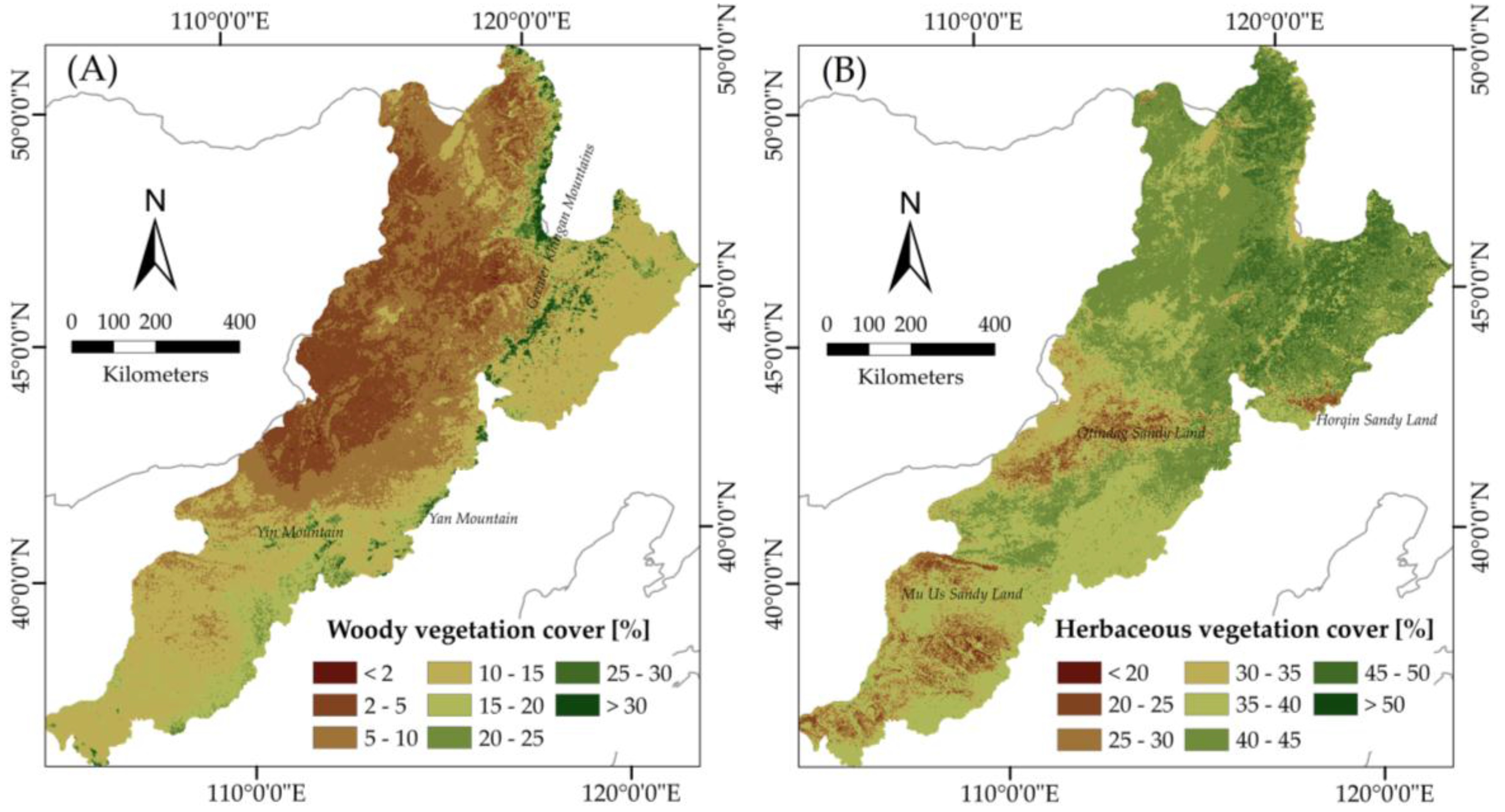
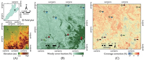
3.2. Mapping Results

The Random Forest models with Sets 8 and 5 were implemented to map fractional cover of woody and herbaceous vegetation in the East Asia Steppe, respectively, for the year 2012, delineated at a 250 m spatial resolution. The estimated map of woody vegetation (Figure 5A) reproduces the woody plant structure of the study area as a heterogeneous mixture of vegetation. Most of the area presents low woody plant density, and woody vegetation coverage between 5% and 15% accounts for more than 65% of the whole study region. High coverage (>20%) of woody plants mainly corresponds to fragmented forests, woodlands, and patchy shrub-lands in mountainous areas located along the eastern and southern parts of the study area (i.e., Greater Khingan Mountains, Yan Mountain, Yin Mountain), which generally has relative high rainfall and soil moisture. Medium coverage (10%–20%) can be found in the traces of dry creek beds most appeared in the north and south. Note that many small patches of woody plants are sparsely distributed in the middle and southwestern part of study area, where the landscape is nature sandy land (i.e., Otindag Sandy Land, Mu Us Sandy Land, Horqin Sandy Land). Herbaceous vegetation (Figure 5B) is characterized by more gradual transition patterns with higher average coverage than woody vegetation. Areas with relatively high herbaceous vegetation coverage (>40%), which correspond mainly to meadow steppe, are generally located at the rim of above mountainous areas, with a mixture of woody plants. Unlike woody estimate, the herbaceous mapping result shows nothing associated with topography, but related with land cover type. For example, the map clearly shows that herbaceous cover obviously decreases with the prevalence of sandy lands (Otindag Sandy Land and Mu Us Sandy land). This spatial distribution also indicates that the influence of sand dunes on vegetation structure can be observed at this spatial resolution.

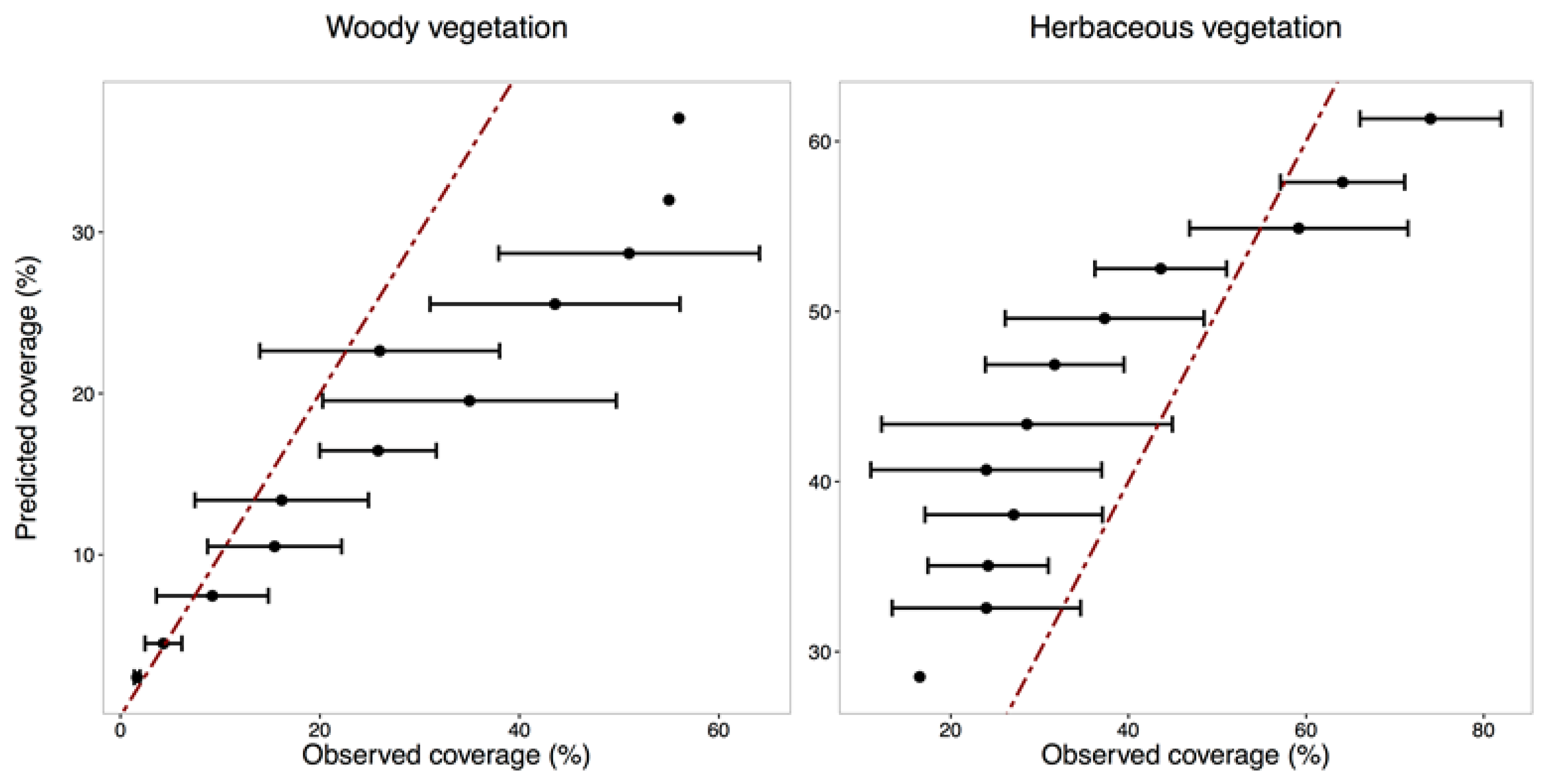
3.3. Validation with Field Data

Figure 6 shows a scatterplot of field measurements versus model results. Although the coverage values are obtained from completely distinct observation means, the plot indicates a consistent agreement between field measurements and estimates within coverage bins. The correlations between these two datasets (Pearson’s r > 0.6) indirectly supported the coverage estimations. In both comparisons, the standard deviation of the field observations fluctuated widely and increased at higher coverage values. In addition to the model conservatism from lowest to highest coverage, an unstable overestimation was also observed in the traditional field investigation results, which were usually subjectively collected in relatively productive vegetation communities over a large area. These results indicated that the models with multiple satellite data as predictor inputs achieved reliable estimates.

4. Discussion

In this woodland to grassland region in East Asia, a quantitative comparison of the woody results with the MODIS-VCF product would be interesting. As shown in Figure 7, the two estimates presented substantially different distribution at low value of fractional woody cover (value < 30%). The MODIS-VCF product includes only trees, while the proposed woody cover estimation in this study can successfully delineate regions with subshrubs, shrubs and scrubs—which is, with respect to semi-arid ecosystems, most meaningful. Hence, the proposed model results in this study suggest that the improved and accurate estimates can be produced based on appropriate predictor inputs and high-quality training data over semi-arid areas.
The goal of this study is to produce improved regional maps of fractional woody and herbaceous vegetation cover that spans the East Asia steppe. The approach that is developed and evaluated for accuracy uses Random Forest by generating training data from high-resolution images and predictor datasets composed of metrics from the MODIS13Q1 product and ancillary variables, including topographic, climatological, and land surface information. The importance of using multiple satellite data as predictor inputs must be stressed. As the point spread function of one sensor is an inevitable limitation in capturing spatial details [30], the integration of multiple satellite data is potentially beneficial for improving estimation performance probably because it may provide more detailed and discernible information of vegetation structures or physiological characteristics. Tree-based approaches calculated only through optical reflection indices, which are less about the terrain and the moisture condition of the land surface, might lead to high inaccuracy in places with low vegetation density and mineral soils [31]. Through the integrating of multiple satellite data, integral model performance might be upgraded over the whole area, and the deviations caused by estimation with or without auxiliary data could be seen as expressing complex regional heterogeneity (Figure 8). Compared with field measurements, model results using only spectral variables tend to overestimate the woody cover on the mountain areas (southeastern part of the region) and underestimate coverage on the high plains (northwestern part of the region). The estimates from models using spectral, topographic, and bio-climatological information are closer to the field values than the spectral data-derived estimates, showing a positive correction with regional heterogeneity.
The importance of achieving highly representative and high-quality training data must be emphasized. In this study, a tailored sampling strategy was implemented to form a spatial sampling layout for improving the representation of training data within each main coverage class. The aim of such specific sampling processing is to obtain results at lower cost, at higher speed, and with greater scope with only a slight loss of accuracy [32]. The theory and applications of spatial sampling techniques have been widely discussed in geoscience [33]. In this study, the similar distributions of sampling results against estimation results suggest the practicability of this multistage sampling procedure. Moreover, training data quality is highly correlated with the approach of image interpretation. As the ability of imaging spectroscopy to provide vegetation signal is limited at low vegetation fractional cover, efforts were made by using a human-machine interactive classification method, which makes it easy to bring technological experience and expertise into the classification process [34]. In this study, in spite of the mean and standard deviation of the confused-pixel proportion for all classified images being relatively low, samples in Zone I and Zone III, which are located in the northern and western parts of the study area, showed relatively high uncertainties in the classification results. These results were mostly caused by the confusion of rich grass and patchy shrubs in the wetter northern region or the misinterpretation between thin grass and bare ground in the drier western region.
As information density expressed at different spatial scales varies greatly [35], whether geospatial information can be used for estimation depends not only on its ability to identify vegetation signal, but also on its spatial resolution. In the final selected dataset, topographical variables (slope, aspect, and elevation) showed less contribution to estimates as we expected (Section 3.1). Although topography has a positive effect on the spatial differentiation of woody vegetation especially in mountain areas [36], this obvious effect may be erased by missing substantial spatial variability at MODIS 250 m resolution in most part of the study area. For herbaceous vegetation, the influence of topography is probably not obvious at this scale due to the wide distribution of this vegetation format. Admittedly, many uncertainties remain regarding the improvement of estimation performance with multiple satellite datasets.
In addition, efforts must be made to minimize their impacts on mapping results because of errors and uncertainties produced during analysis are inevitably propagated. During training data preparation and predictor variables pre-processing, pixel georeferencing errors (i.e., inherent geolocation errors, projection errors) could cause spatial mismatch between training and predictor data. Any spatial shift between different datasets could cause a change of value at corresponding locations. Therefore, the size of the sample grid has been slightly expanded and all the predictor variables have been transformed into a database with unified units. In this study, nonparametric regressive models were constructed to make estimates more robust to predictor data noise. Despite the truth that errors caused by tree-based algorithms generally contribute the most to the total errors, which were translated into degraded model performance and estimation accuracy [37], the optimal models were selected on the basis of the invariant indicators of model performance to reduce their impacts on mapping results.

5. Conclusions

This study presents regional maps of fractional woody and herbaceous vegetation cover in a large semi-arid steppe across China, Mongolia, and Russia. The approach is developed using Random Forest with combined multiple remote sensing data—training samples derived from high-resolution images in a tailored spatial sampling—and model inputs composed of specific MODIS metrics and ancillary variables cast onto the same grid. The optimal models used for mapping are selected from several RF models with different predictor sets based on performance evaluation. An independent validation set of ground observation plots is used to assess the accuracy of selected RF models. The mapping results in East Asia steppe show that improved cover estimates could be produced with high-quality training samples and appropriate model inputs. It is stressed here that effective spatial sampling, high-quality classification, and adequate geospatial information are important prerequisites to establishing optimal models for mapping.
This approach could be applicable over sizable semi-arid areas with mixed vegetation mosaics and gradual transitions. This could provide improved estimates of vegetation cover information not only for temperate steppes, but also for similar semi-arid biomes, such as savannas and prairies. This study demonstrates that the combination of geospatial information from multiple satellite data improves the correlation between remote sensing observations and vegetation characteristic signals. Given the uncertainties produced from estimating process including training data generation, predictor variable pre-processing and algorithm implementation, it can be expected that the integration of more remote sensing observations and nonparametric simulation methods becomes more critical to make further improvements on model performance and accuracy of woody and herbaceous vegetation estimation.

Acknowledgments

This research was granted by National Natural Science Foundation of China (NSFC 41325002 and 41530747) and National Key Research and Development Program (2016YFC0500701).

Author Contributions

Xu Liu and Hongyan Liu conceived and designed the experiments; Xu Liu performed the experiments; Xu Liu and Hongyan Liu analyzed the data; Shuang Qiu contributed reagents/materials/analysis tools; Xu Liu wrote the paper; Xiuchen Wu, Yuhong Tian and Qian Hao revised the paper.

Conflicts of Interest

The authors declare no conflict of interest.

References

  1. DeFries, R.; Achard, F.; Brown, S.; Herold, M.; Murdiyarso, D.; Schlamadinger, B.; de Souza, C. Earth observations for estimating greenhouse gas emissions from deforestation in developing countries. Environ. Sci. Policy 2007, 10, 385–394. [Google Scholar] [CrossRef]
  2. Yang, J.; Weisberg, P.J.; Bristow, N.A. Landsat remote sensing approaches for monitoring long-term tree cover dynamics in semi-arid woodlands: Comparison of vegetation indices and spectral mixture analysis. Remote Sens. Environ. 2012, 119, 62–71. [Google Scholar] [CrossRef]
  3. Harris, A.; Carr, A.S.; Dash, J. Remote sensing of vegetation cover dynamics and resilience across southern Africa. Int. J. Appl. Earth Observ. Geoinf. 2014, 28, 131–139. [Google Scholar] [CrossRef]
  4. Liu, H.; Cui, H.; Pott, R.; Speier, M. Vegetation of the woodland-steppe transition at the southeastern edge of the Inner Mongolian Plateau. J. Veg. Sci. 2000, 11, 525–532. [Google Scholar] [CrossRef]
  5. Archer, S. Tree-grass dynamics in a thornscrub savanna parkland: Reconstructing the past and predicting the future. Ecoscience 2016, 2, 83–99. [Google Scholar] [CrossRef]
  6. Yu, K.; D’Odorico, P. Hydraulic lift as a determinant of tree-grass coexistence on savannas. New Phytol. 2015, 207, 1038–1051. [Google Scholar] [CrossRef] [PubMed]
  7. Brazier, R.E.; Turnbull, L.; Wainwright, J.; Bol, R. Carbon loss by water erosion in drylands: Implications from a study of vegetation change in the south-west USA. Hydrol. Process. 2014, 28, 2212–2222. [Google Scholar] [CrossRef] [Green Version]
  8. Sitch, S.; Friedlingstein, P.; Gruber, N.; Jones, S.D.; Murray-Tortarolo, G.; Ahlström, A.; Doney, S.C.; Graven, H.; Heinze, C.; Huntingford, C.; et al. Recent trends and drivers of regional sources and sinks of carbon dioxide. Biogeosciences 2015, 12, 653–679. [Google Scholar] [CrossRef] [Green Version]
  9. Elmendorf, S.C. Global assessment of experimental climate warming on tundra vegetation: Heterogeneity over space and time. Ecol. Lett. 2014, 15, 164–175. [Google Scholar] [CrossRef] [PubMed]
  10. Gessner, U.; Machwitz, M.; Conrad, C.; Dech, S. Estimating the fractional cover of growth forms and bare surface in savannas. A multi-resolution approach based on regression tree ensembles. Remote Sens. Environ. 2013, 129, 90–102. [Google Scholar] [CrossRef] [Green Version]
  11. Okin, G.S.; Clarke, K.D.; Lewis, M.M. Comparison of methods for estimation of absolute vegetation and soil fractional cover using modis normalized brdf-adjusted reflectance data. Remote Sens. Environ. 2013, 130, 266–279. [Google Scholar] [CrossRef]
  12. Fluet-Chouinard, E.; Lehner, B.; Rebelo, L.M.; Papa, F.; Hamilton, S.K. Development of a global inundation map at high spatial resolution from topographic downscaling of coarse-scale remote sensing data. Remote Sens. Environ. 2015, 158, 348–361. [Google Scholar] [CrossRef]
  13. Mishra, N.B.; Crews, K.A.; Okin, G.S. Relating spatial patterns of fractional land cover to savanna vegetation morphology using multi-scale remote sensing in the Central Kalahari. Int. J. Remote Sens. 2014, 35, 2082–2104. [Google Scholar]
  14. Brandt, M.; Hiernaux, P.; Tagesson, T.; Verger, A.; Rasmussen, K.; Diouf, A.A.; Mbow, C.; Mougin, E.; Fensholt, R. Woody plant cover estimation in drylands from Earth Observation based seasonal metrics. Remote Sens. Environ. 2016, 172, 28–38. [Google Scholar] [CrossRef]
  15. DiMiceli, C.M.; Carroll, M.L.; Sohlberg, R.A.; Huang, C.; Hansen, M.C.; Townshend, J.R.G. Annual Global Automated MODIS Vegetation Continuous Fields (MOD44B) at 250 m Spatial Resolution for Data Years Beginning Day 65, 2000–2010, Collection 5 Percent Tree Cover; University of Maryland: College Park, MD, USA, 2011. [Google Scholar]
  16. Medina, E.; Cuevas, E.; Molina, S.; Luco, A.E.; Ramos, O. Structural variability and species diversity of a dwarf caribbean dry forest. Caribb. J. Sci. 2012, 46, 203–215. [Google Scholar] [CrossRef]
  17. Ma, L.; Zhou, Y.; Chen, J.; Cao, X.; Chen, X.H. Estimation of fractional vegetation cover in semiarid areas by integrating endmember reflectance purification into nonlinear spectral mixture analysis. IEEE Geosci. Remote Sens. 2015, 12, 1175–1179. [Google Scholar]
  18. Chopping, M.; Su, L.; Rango, A.; Martonchik, J.V.; Peters, D.P.C.; Laliberte, A. Remote sensing of woody shrub cover in desert grasslands using MISR with a geometric-optical canopy reflectance model. Remote Sens. Environ. 2008, 112, 19–34. [Google Scholar] [CrossRef]
  19. Johnson, B.; Tateishi, R.; Kobayashi, T. Remote sensing of fractional green vegetation cover using spatially-interpolated endmembers. Remote Sens. 2012, 4, 2619–2634. [Google Scholar] [CrossRef]
  20. Brown, J.F.; Howard, D.; Wylie, B.; Frieze, A.; Ji, L.; Gacke, C. Application-ready expedited MODIS data for operational land surface monitoring of vegetation condition. Remote Sens. 2015, 7, 16226–16240. [Google Scholar] [CrossRef]
  21. Hansen, M.C.; Townshend, J.R.G.; Defries, R.S.; Carroll, M. Estimation of tree cover using modis data at global, continental and regional/local scales. Int. J. Remote Sens. 2005, 26, 4359–4380. [Google Scholar] [CrossRef]
  22. Yin, Y.; Liu, H.Y.; He, S.Y.; Zhao, F.J.; Zhu, J.L.; Wang, H.Y.; Liu, G.; Wu, X.C. Patterns of local and regional grain size distribution and their application to holocene climate reconstruction in semi-arid Inner Mongolia, China. Palaeogeogr. Palaeoclimatol. Palaeoecol. 2011, 307, 168–176. [Google Scholar] [CrossRef]
  23. Clark, M.L.; Aide, T.M.; Grau, H.R.; Riner, G. A scalable approach to mapping annual land cover at 250 m using MODIS time series data: A case study in the Dry Chaco ecoregion of South America. Remote Sens. Environ. 2010, 114, 2816–2832. [Google Scholar] [CrossRef]
  24. Avitabile, V.; Baccini, A.; Friedl, M.A.; Schmullius, C. Capabilities and limitations of landsat and land cover data for aboveground woody biomass estimation of Uganda. Remote Sens. Environ. 2012, 117, 366–380. [Google Scholar] [CrossRef]
  25. Peters, D. Future Directions in Jornada Research: Applying an Interactive Landscape Model to Solve Problems. In Structure and Function of a Chihuahuan Desert Ecosystem: The Jornada Basin Long-Term Ecological Research Site; Oxford University Press: New York, NY, USA, 2006. [Google Scholar]
  26. Liu, H.Y.; He, S.Y.; Anenkhonov, O.A.; Hu, G.Z.; Sandanov, D.V.; Badmaeva, N.K. Topography-controlled soil water content and the coexistence of forest and steppe in Northern China. Phys. Geogr. 2012, 33, 561–573. [Google Scholar] [CrossRef]
  27. Liu, S.L.; Wang, T.; Guo, J.; Qu, J.J.; An, P.J. Vegetation change based on SPOT-VGT data from 1998–2007, northern China. Environ. Earth Sci. 2010, 60, 1459–1466. [Google Scholar] [CrossRef]
  28. Sternberg, T. Piospheres and pastoralists: Vegetation and degradation in steppe grasslands. Hum. Ecol. 2012, 40, 811–820. [Google Scholar] [CrossRef]
  29. Bai, Y.F.; Han, X.G.; Wu, J.G.; Chen, Z.Z.; Li, L.H. Ecosystem stability and compensatory effects in the Inner Mongolia grassland. Nature 2004, 431, 181–184. [Google Scholar] [CrossRef] [PubMed]
  30. Clark, M.L.; Roberts, D.A.; Ewel, J.J.; Clark, D.B. Estimation of tropical rain forest aboveground biomass with small-footprint lidar and hyperspectral sensors. Remote Sens. Environ. 2011, 115, 2931–2942. [Google Scholar] [CrossRef]
  31. Oh, Y.; Kwon, S.G.; Hwang, J.H. Soil moisture detection using kompsat-5 sar data. In Proceedings of the 2010 IEEE International Geoscience and Remote Sensing Symposium (IGARSS), Honolulu, HI, USA, 25–30 July 2010; pp. 1250–1253.
  32. Wang, J.F.; Christakos, G.; Hu, M.G. Modeling spatial means of surfaces with stratified nonhomogeneity. IEEE Trans. Geosci. Remote Sens. 2009, 47, 4167–4174. [Google Scholar] [CrossRef]
  33. Christakos, G. Methodological developments in geophysical assimilation modeling. Rev. Geophys. 2005, 43. [Google Scholar] [CrossRef]
  34. Daschiel, H.; Datcu, M. Information mining in remote sensing image archives: System evaluation. IEEE Trans. Geosci. Remote Sens. 2005, 43, 188–199. [Google Scholar] [CrossRef]
  35. Lindgren, K. An information-theoretic perspective on coarse-graining, including the transition from micro to macro. Entropy 2015, 17, 3332–3351. [Google Scholar] [CrossRef]
  36. Yang, W.Z.; Ni-Meister, W.; Lee, S. Assessment of the impacts of surface topography, off-nadir pointing and vegetation structure on vegetation lidar waveforms using an extended geometric optical and radiative transfer model. Remote Sens. Environ. 2011, 115, 2810–2822. [Google Scholar] [CrossRef]
  37. Doerr, D.; Gronau, I.; Moran, S.; Yavneh, I. Stochastic errors vs. modeling errors in distance based phylogenetic reconstructions. Algorithms Mol. Biol. 2012, 7. [Google Scholar] [CrossRef] [PubMed]
Figure 1. Location and topography of the East Asia steppe, with the grid of corresponding MODIS tiles and the site of the field survey (black triangle).
Remotesensing 09 00032 g001
Figure 2. Simple workflow of mapping woody and herbaceous fractional cover in the East Asia steppe. The whole procedure consists of three parts: I.) predictor data pre-processing; II.) training data preparation; and III.) model estimation.
Remotesensing 09 00032 g002
Figure 3. (A) Layout of spatial sampling, with the zones (four colors, by domain knowledge), primary grid cells (grey rectangle), and final sample locations (black cross); (B) in each sampling grid, the actual locations of the final samples were selected based on both systematic sampling results and land surface conditions; and (C) each final sample was generated along with a 10 × 10 internal net of predictor units (black rectangle, similar to MODIS 250 m pixel), and GE images with a size slightly larger than 2.5 km were used here as reference data of vegetation covers.
Remotesensing 09 00032 g003
Figure 4. Layout of plots with five-quadrant modes for field measurement of vegetation covers. Each plot consisted of five smaller quadrants with sizes as close as 50 m × 50 m for each one. Plant parameters, including cover fractions, were surveyed on the ground by averaging two or three observations from transects along the landscape terrain within each quadrat. To match the size of predictor units, plots were designed to be slightly larger than 250 m × 250 m, or with a total area more than 60,000 m2.
Remotesensing 09 00032 g004
Figure 5. Fractional coverage map of (A) woody vegetation and (B) herbaceous vegetation for the East Asia steppe (2012 growing season).
Remotesensing 09 00032 g005
Figure 6. Comparison between field measurements and model estimations. The horizontal bars represent standard errors for field surveys within coverage bins.
Remotesensing 09 00032 g006
Figure 7. The density distributions of our predicted values (red area) and MIDOS-VCF product values (blue area). They show significant difference in relative low woody coverage value (<30%) represented by the dark part of the figure. From the lowest to the highest proportion of woody cover, the main landscape possibly changes from grassland with rare subshrub to open forest.
Remotesensing 09 00032 g007
Figure 8. Example of estimation improvement using models with combined input datasets. (A) Locations of field observation sites in various terrains; (B) the spectral data-derived estimation of woody cover; (C) the correction of estimation calculated through the optimal model (with combined input sets) results minus the values shown in (B). The model result Remotesensing 09 00032 i001 overestimates, Remotesensing 09 00032 i002 underestimates, and Remotesensing 09 00032 i003 
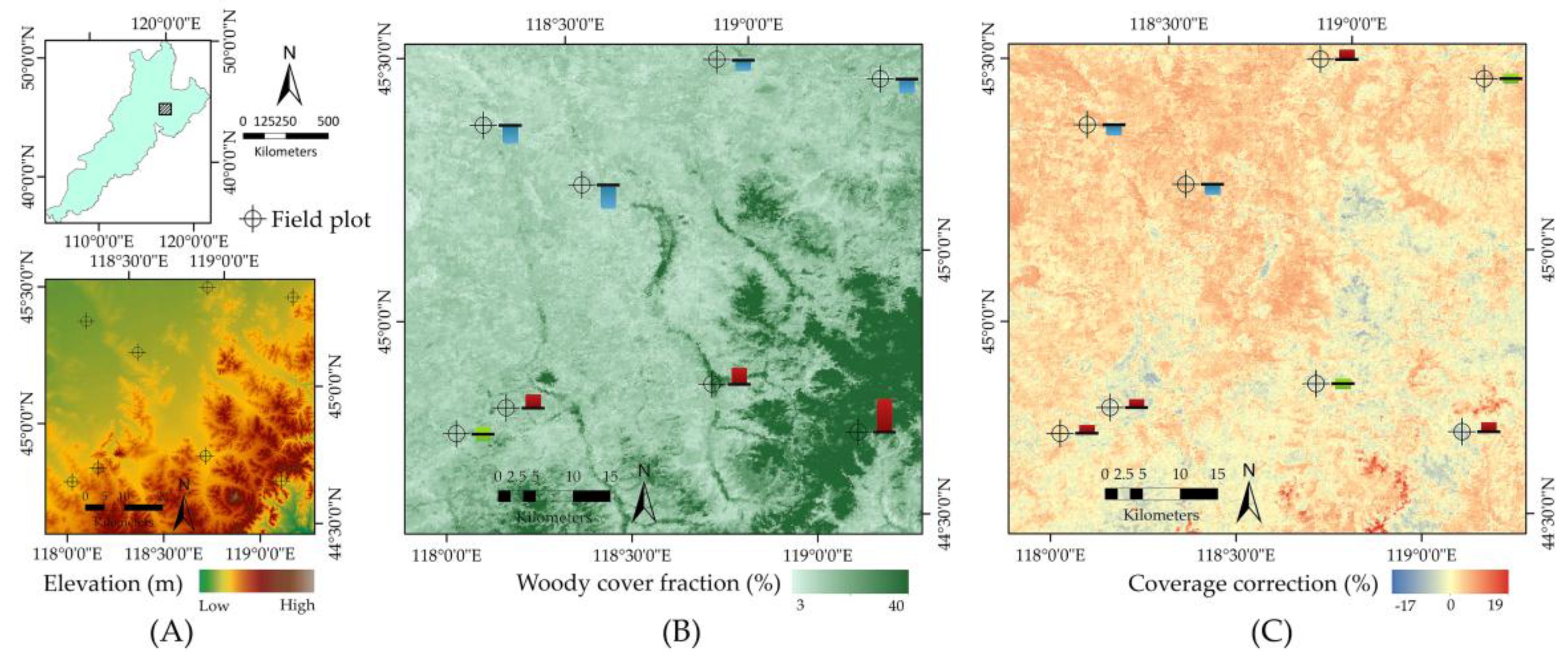
is as close to the woody cover fraction observed in the field. We can see that the optimal model results are closer to field values and the correction for deviation express regional heterogeneity.
Remotesensing 09 00032 g008
Table 1. The brief introduce of each type of predictor variables and corresponding resampling method.
TypeVariablesBrief IntroductionSourceOriginal Spatial Resolution
Vegetation IndexNDVI/EVIRepresent growing conditions of plantsLP DAAC MODIS 13Q1250 m
Optical ReflectanceBlue/red/NIR/MIRUsed to distinguish the features of vegetation and non-vegetation250 m
Bioclimatic variablesTemperature/precipitation statisticsProvide annual trends, seasonality and extreme environmental factorsWorldclim data library30 arc seconds (≈1 km)
Topographic InformationelevationRepresent micro-relief conditions of plantsCGIAR-CSI STRM 90 m DEM3 arc seconds (≈90 m)
slope/aspectIIASA-Global Terrain Slope and Aspect Data30 arc seconds
Land Surface Informationsoil typeProvide plant forms and vegetation phenology informationHarmonized World Soil Database (HWSD)30 arc seconds
land cover typeESA GlobCover300 m
Table 2. Performance statistics derived from Random Forest models. The combination of absolute deviation and normalized mean square error (NMSE) indicates the estimation accuracy of models with different input datasets.
Variable SetWoody VegetationHerbaceous Vegetation
BiasNMSEBiasNMSE
Set 1: vegetation and reflectance indices0.650.5602.090.772
Set 2: Set 1 + land-cover and soil type0.810.5392.180.745
Set 3: Set 1 + bioclimatic variables0.850.4951.210.658
Set 4: Set 1 + topographic variables0.800.5740.740.710
Set 5: Set 2 + bioclimatic variables0.530.4910.780.643
Set 6: Set 2 + topographic variables0.860.5321.050.700
Set 7: Set 3 + topographic variables0.440.4910.680.683
Set 8: All variables0.420.4690.720.650
Table 3. The counts and summed scores of predictor variable importance for each data type. The types of variables with higher values are considered to be more important for estimation.
Variable TypeWoody VegetationHerbaceous Vegetation
Optical reflectance (20)109.3114.8
Vegetation index (10)53.484.5
Bioclimatic information (19)126.6137.9
Topographic information (5)22.8-
Land surface information (2)11.33.12

