
Potential of ALOS2 and NDVI to Estimate Forest Above-Ground Biomass, and Comparison with Lidar-Derived Estimates

 ,
,  ,
, 
 , , and
Abstract
:
1. Introduction
2. Materials and Methods
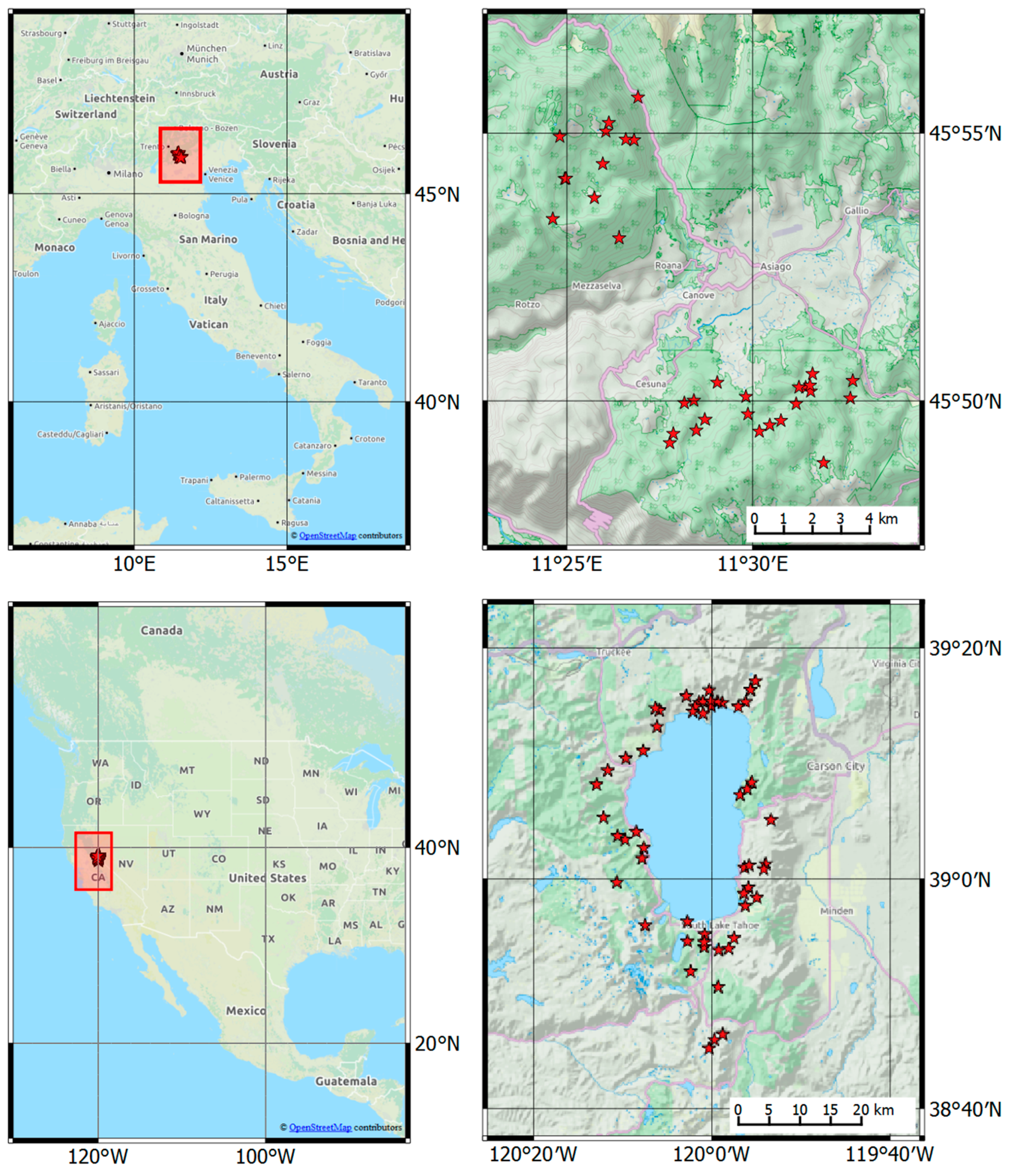
2.1. Field Data
2.2. Remote Sensing Data
2.3. Lidar Data and Derived AGB Maps
2.4. Data Analysis
- the SAR statistics (minimum, maximum, mean, standard deviation per HH and HV; HH and HV sum and difference; total 10 inputs);
- the SAR statistics plus SAR-GLCM textures per HH and HV (total 26 inputs);
- the SAR statistics plus NDVI and NDVI-GLCM textures (total 19 inputs);
- SAR HH + HV selected by Test 1 plus the SAR-GLCM texture type selected by Test 2 and the NDVI feature type selected by Test 3 (totaling three inputs).
3. Results
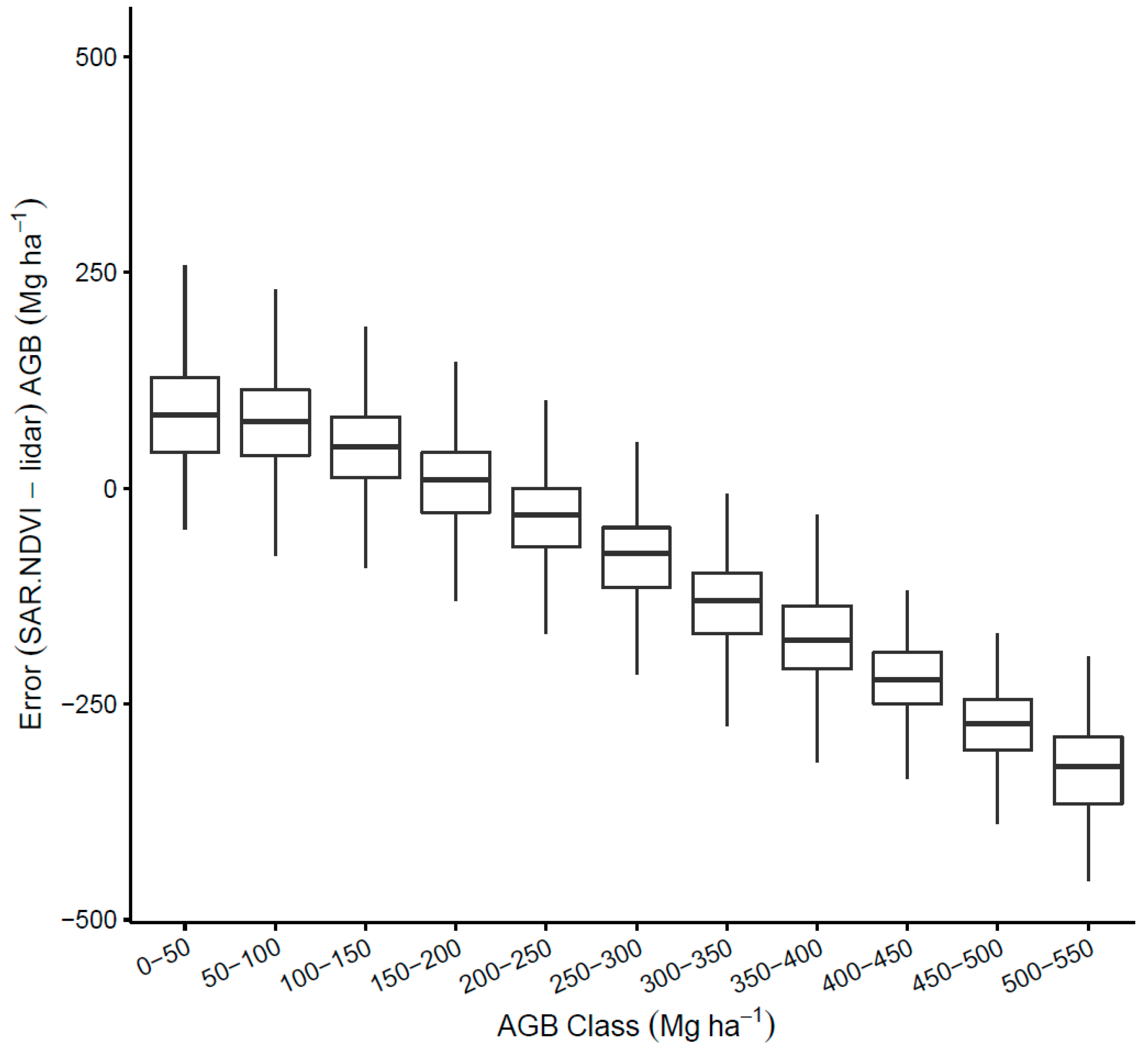
4. Discussion
5. Conclusions
Acknowledgments
Author Contributions
Conflicts of Interest
References
- Dixon, R.; Brown, S.; Houghton, R.E.A.; Solomon, A.M.; Trexler, M.C.; Wisniewski, J. Carbon pools and flux of global forest ecosystems. Science 1994, 263, 185–189. [Google Scholar] [CrossRef] [PubMed]
- Strassburg, B.B.N.; Kelly, A.; Balmford, A.; Davies, R.G.; Gibbs, H.K.; Lovett, A.; Miles, L.; Orme, C.D.L.; Price, J.; Turner, R.K.; et al. Global congruence of carbon storage and biodiversity in terrestrial ecosystems. Conserv. Lett. 2010, 3, 98–105. [Google Scholar] [CrossRef]
- Turner, W.; Spector, S.; Gardiner, N.; Fladeland, M.; Sterling, E.; Steininger, M. Remote sensing for biodiversity science and conservation. Trends Ecol. Evol. 2003, 18, 306–314. [Google Scholar] [CrossRef]
- Lu, D.; Chen, Q.; Wang, G.; Liu, L.; Li, G.; Moran, E. A survey of remote sensing-based aboveground biomass estimation methods in forest ecosystems. Int. J. Digit. Earth 2016, 9, 63–105. [Google Scholar] [CrossRef]
- Clark, M.L.; Roberts, D.A.; Ewel, J.J.; Clark, D.B. Estimation of tropical rain forest aboveground biomass with small-footprint lidar and hyperspectral sensors. Remote Sens. Environ. 2011, 115, 2931–2942. [Google Scholar] [CrossRef]
- Chen, Q. Lidar remote sensing of vegetation biomass. Remote Sens. Nat. Resour. 2013, 399, 399–420. [Google Scholar]
- Chen, Q.; Laurin, G.V.; Battles, J.J.; Saah, D. Integration of airborne lidar and vegetation types derived from aerial photography for mapping aboveground live biomass. Remote Sens. Environ. 2012, 121, 108–117. [Google Scholar] [CrossRef]
- Naesset, E. Estimating timber volume of forest stands using airborne laser scanner data. Remote Sens. Environ. 1997, 61, 246–253. [Google Scholar] [CrossRef]
- Lu, D.; Chen, Q.; Wang, G.; Moran, E.; Batistella, M.; Zhang, M.; Vaglio Laurin, G.; Saah, D. Aboveground forest biomass estimation with Landsat and LiDAR data and uncertainty analysis of the estimates. Int. J. For. Res. 2012, 2012, 1–16. [Google Scholar] [CrossRef]
- Patenaude, G.; Hill, R.A.; Milne, R.; Gaveau, D.L.A.; Briggs, B.B.J.; Dawson, T.P. Quantifying forest above ground carbon content using LiDAR remote sensing. Remote Sens. Environ. 2004, 93, 368–380. [Google Scholar] [CrossRef]
- Riom, J.; Le Toan, T. Relation entre des types de forets de pin maritime et la retrodiffusion radar en bande L. en polarisation HH.[teledetection]. Colloq. l’INRA (France) 1981, 5. [Google Scholar]
- Tanase, M.A.; Panciera, R.; Lowell, K.; Tian, S.; Garcia-Martin, A.; Walker, J.P. Sensitivity of L-band radar backscatter to forest biomass in semiarid environments: A comparative analysis of parametric and nonparametric models. IEEE Trans. Geosci. Remote Sens. 2014, 52, 4671–4685. [Google Scholar] [CrossRef]
- Dobson, M.C.; Ulaby, F.T.; LeToan, T.; Beaudoin, A.; Kasischke, E.S.; Christensen, N. Dependence of radar backscatter on coniferous forest biomass. IEEE Trans. Geosci. Remote Sens. 1992, 30, 412–415. [Google Scholar] [CrossRef]
- Le Toan, T.; Quegan, S.; Davidson, M.W.J.; Balzter, H.; Paillou, P.; Papathanassiou, K.; Plummer, S.; Rocca, F.; Saatchi, S.; Shugart, H.; et al. The BIOMASS mission: Mapping global forest biomass to better understand the terrestrial carbon cycle. Remote Sens. Environ. 2011, 115, 2850–2860. [Google Scholar] [CrossRef]
- Cartus, O.; Santoro, M.; Kellndorfer, J. Mapping forest aboveground biomass in the Northeastern United States with ALOS PALSAR dual-polarization L-band. Remote Sens. Environ. 2012, 124, 466–478. [Google Scholar] [CrossRef]
- Harrell, P.A.; Bourgeau-Chavez, L.L.; Kasischke, E.S.; French, N.H.F.; Christensen, N.L. Sensitivity of ERS-1 and JERS-1 radar data to biomass and stand structure in Alaskan boreal forest. Remote Sens. Environ. 1995, 54, 247–260. [Google Scholar] [CrossRef]
- Saatchi, S.; Marlier, M.; Chazdon, R.L.; Clark, D.B.; Russell, A.E. Impact of spatial variability of tropical forest structure on radar estimation of aboveground biomass. Remote Sens. Environ. 2011, 115, 2836–2849. [Google Scholar] [CrossRef]
- Santoro, M.; Eriksson, L.; Askne, J.; Schmullius, C. Assessment of stand-wise stem volume retrieval in boreal forest from JERS-1 L-band SAR backscatter. Int. J. Remote Sens. 2006, 27, 3425–3454. [Google Scholar] [CrossRef]
- Santos, J.R.; Lacruz, M.S.P.; Araujo, L.S.; Keil, M. Savanna and tropical rainforest biomass estimation and spatialization using JERS-1 data. Int. J. Remote Sens. 2002, 23, 1217–1229. [Google Scholar] [CrossRef]
- Lucas, R.; Armston, J.; Fairfax, R.; Fensham, R.; Accad, A.; Carreiras, J.; Kelley, J.; Bunting, P.; Clewley, D.; Bray, S.; et al. An evaluation of the ALOS PALSAR L-band backscatter—Above ground biomass relationship Queensland, Australia: Impacts of surface moisture condition and vegetation structure. IEEE J. Sel. Top. Appl. Earth Obs. Remote Sens. 2010, 3, 576–593. [Google Scholar] [CrossRef]
- Carreiras, J.; Melo, J.B.; Vasconcelos, M.J. Estimating the above-ground biomass in miombo savanna woodlands (Mozambique, East Africa) using L-band synthetic aperture radar data. Remote Sens. 2013, 5, 1524–1548. [Google Scholar] [CrossRef]
- Imhoff, M.L. A theoretical analysis of the effect of forest structure on synthetic aperture radar backscatter and the remote sensing of biomass. IEEE Trans. Geosci. Remote Sens. 1995, 33, 341–352. [Google Scholar] [CrossRef]
- Le Toan, T.; Quegan, S.; Woodward, I.; Lomas, M.; Delbart, N.; Picard, G. Relating radar remote sensing of biomass to modelling of forest carbon budgets. Clim. Chang. 2004, 67, 379–402. [Google Scholar] [CrossRef]
- Saatchi, S.; Halligan, K.; Despain, D.G.; Crabtree, R.L. Estimation of forest fuel load from radar remote sensing. IEEE Trans. Geosci. Remote Sens. 2007, 45, 1726–1740. [Google Scholar] [CrossRef]
- Sandberg, G.; Ulander, L.M.H.; Fransson, J.E.S.; Holmgren, J.; Le Toan, T. L-and P-band backscatter intensity for biomass retrieval in hemiboreal forest. Remote Sens. Environ. 2011, 115, 2874–2886. [Google Scholar] [CrossRef]
- He, Q.-S.; Cao, C.-X.; Chen, E.-X.; Sun, G.-Q.; Ling, F.-L.; Pang, Y.; Zhang, H.; Ni, W.-J.; Xu, M.; Li, Z.-Y.; et al. Forest stand biomass estimation using ALOS PALSAR data based on LiDAR-derived prior knowledge in the Qilian Mountain, western China. Int. J. Remote Sens. 2012, 33, 710–729. [Google Scholar] [CrossRef]
- Michelakis, D.G.; Stuart, N.; Woodhouse, I.H.; Lopez, G.; Linares, V. Establishing the sensitivity of ALOS PALSAR to above ground woody biomass: A case study in the pine savannas of Belize, Central America. In Proceedings of the 2013 IEEE International Geoscience and Remote Sensing Symposium (IGARSS), Melbourne, Australia, 21–26 July 2013; pp. 953–956.
- Hansen, E.H.; Gobakken, T.; Bollandsås, O.M.; Zahabu, E.; Næsset, E. Modeling aboveground biomass in dense tropical submontane rainforest using airborne laser scanner data. Remote Sens. 2015, 7, 788–807. [Google Scholar] [CrossRef]
- Sarker, L.R.; Nichol, J.; Iz, H.B.; Ahmad, B.B.; Rahman, A.A. Forest biomass estimation using texture measurements of high-resolution dual-polarization C-band SAR data. IEEE Trans. Geosci. Remote Sens. 2013, 51, 3371–3384. [Google Scholar] [CrossRef]
- Haralick, R.M. Statistical and structural approaches to texture. Proc. IEEE 1979, 67, 786–804. [Google Scholar] [CrossRef]
- Attarchi, S.; Gloaguen, R. Improving the estimation of above ground biomass using dual polarimetric PALSAR and ETM+ data in the Hyrcanian Mountain Forest (Iran). Remote Sens. 2014, 6, 3693–3715. [Google Scholar] [CrossRef]
- Champion, I.; Da Costa, J.P.; Godineau, A.; Villard, L.; Dubois-Fernandez, P.; Le Toan, T. Canopy structure effect on SAR image texture versus forest biomass relationships. EARSeL eProc. 2013, 12. [Google Scholar] [CrossRef]
- Deng, S.; Katoh, M.; Guan, Q.; Yin, N.; Li, M. Estimating forest aboveground biomass by combining ALOS PALSAR and WorldView-2 data: A case study at Purple Mountain National Park, Nanjing, China. Remote Sens. 2014, 6, 7878–7910. [Google Scholar] [CrossRef]
- Basuki, T.M.; Skidmore, A.K.; Hussin, Y.A.; Van Duren, I. Estimating tropical forest biomass more accurately by integrating ALOS PALSAR and Landsat-7 ETM+ data. Int. J. Remote Sens. 2013, 34, 4871–4888. [Google Scholar] [CrossRef]
- Fedrigo, M.; Meir, P.; Sheil, D.; Van Heist, M.; Woodhouse, I.H.; Mitchard, E.T.A. Fusing radar and optical remote sensing for biomass prediction in mountainous tropical forests. In Proceedings of the 2013 IEEE International Geoscience and Remote Sensing Symposium (IGARSS), Melbourne, Australia, 21–26 July 2013; pp. 975–978.
- Azcueta, M.; d’Alessandro, M.M.; Zajc, T.; Grunfeld, N.; Thibeault, M. ALOS-2 preliminary calibration assessment. In Proceedings of the 2015 IEEE International Geoscience and Remote Sensing Symposium (IGARSS), Milan, Italy, 26–31 July 2015; pp. 4117–4120.
- Rosenqvist, A.; Shimada, M.; Suzuki, S.; Ohgushi, F.; Tadono, T.; Watanabe, M.; Tsuzuku, K.; Watanabe, T.; Kamijo, S.; Aoki, E. Operational performance of the ALOS global systematic acquisition strategy and observation plans for ALOS-2 PALSAR-2. Remote Sens. Environ. 2014, 155, 3–12. [Google Scholar] [CrossRef]
- Nguyen, L.V.; Tateishi, R.; Nguyen, H.T.; Sharma, R.C.; To, T.T.; Le, S.M. Estimation of tropical forest structural characteristics using ALOS-2 SAR data. Adv. Remote Sens. 2016, 5, 131–144. [Google Scholar] [CrossRef]
- Tabacchi, G.; Di Cosmo, L.; Gasparini, P. Aboveground tree volume and phytomass prediction equations for forest species in Italy. Eur. J. For. Res. 2011, 130, 911–934. [Google Scholar] [CrossRef]
- Tabacchi, G.; Di Cosmo, L.; Gasparini, P.; Morelli, S. Stima del volume e della fitomassa delle principali specie forestali italiane. Equazioni di previsione, tavole del volume e tavole della fitomassa arborea epigea. Consiglio per la Ricerca e la sperimentazione in Agricoltura, Unit{à} di Ricerca per il Moni. In Trento: Consiglio per la Ricerca e la Sperimentazione in Agricoltura, Unita di Ricerca per il Monitoraggio e la Pianificazione Forestale; Consiglio per la Ricerca e la sperimentazione in Agricoltura (CRA): Roma, Italy, 2011. (In Italian) [Google Scholar]
- Chen, Q. Modeling aboveground tree woody biomass using national-scale allometric methods and airborne lidar. ISPRS J. Photogramm. Remote Sens. 2015, 106, 95–106. [Google Scholar] [CrossRef]
- White, A.; Manley, P. Wildlife Habitat Occurrence Models for Project and Landscape Evaluations in the Lake Tahoe Basin. Final Report to the U.S. Department of Interior, Bureau of Land Management. 2012. Available online: https://www.fs.fed.us/psw/partnerships/tahoescience/documents/p050_FinalReportWildlifeHabitat.pdf (accessed on 23 December 2016).
- Heath, L.S.; Hansen, M.; Smith, J.E.; Miles, P.D.; Smith, B.W. Investigation into calculating tree biomass and carbon in the FIADB using a biomass expansion factor approach. In Proceedings of the Forest Inventory and Analysis (FIA) Symposium 2008, Park City, UT, USA, 21–23 October 2008; U.S. Department of Agriculture, Forest Service, Rocky Mountain Research Station: Fort Collins, CO, USA, 2009. [Google Scholar]
- Woodall, C.W.; Heath, L.S.; Domke, G.M.; Nichols, M.C. Methods and equations for estimating aboveground volume, biomass, and carbon for trees in the US forest inventory, 2010. In General Technical Report NRS-88; U.S. Department of Agriculture, Forest Service, Northern Research Station: Newtown Square, PA, USA, 2011. [Google Scholar]
- ALOS-2/Calibration Result of JAXA Standard Products. Available online: http://www.eorc.jaxa.jp/ALOS-2/en/calval/calval_index.htm (accessed on 6 December 2015).
- Chen, Q. Airborne lidar data processing and information extraction. Photogramm. Eng. Remote Sens. 2007, 73, 109–112. [Google Scholar]
- Pirotti, F.; Guarnieri, A.; Vettore, A. Analysis of correlation between full-waveform metrics, scan geometry and land-cover: An application over forests. ISPRS Ann. Photogramm. Remote Sens. Spat. Inf. Sci. 2013, II-5/W2, 235–240. [Google Scholar] [CrossRef]
- Matlab, version 2010b; MathWorks Inc.: Natick, MA, USA, 2012.
- RC Team. R: A Language and Environment for Statistical Computing, R Foundation for Statistical Computing: Vienna, Austria, 2013.
- Zolkos, S.G.; Goetz, S.J.; Dubayah, R. A meta-analysis of terrestrial aboveground biomass estimation using lidar remote sensing. Remote Sens. Environ. 2013, 128, 289–298. [Google Scholar] [CrossRef]
- Chen, Q.; Laurin, G.V.; Valentini, R. Uncertainty of remotely sensed aboveground biomass over an African tropical forest: Propagating errors from trees to plots to pixels. Remote Sens. Environ. 2015, 160, 134–143. [Google Scholar] [CrossRef]
- Tanase, M.A.; Panciera, R.; Lowell, K.; Aponte, C.; Hacker, J.M.; Walker, J.P. Forest biomass estimation at high spatial resolution: Radar versus lidar sensors. IEEE Geosci. Remote Sens. Lett. 2014, 11, 711–715. [Google Scholar] [CrossRef]
- Goh, J.; Miettinen, J.; Chia, A.S.; Chew, P.T.; Liew, S.C. Biomass estimation in humid tropical forest using a combination of ALOS PALSAR and SPOT 5 satellite imagery. Asian J. Geoinform. 2014, 13. [Google Scholar]
- Bharadwaj, P.S.; Kumar, S.; Kushwaha, S.P.S.; Bijker, W. Polarimetric scattering model for estimation of above ground biomass of multilayer vegetation using ALOS-PALSAR quad-pol data. Phys. Chem. Earth Parts A/B/C 2015, 83, 187–195. [Google Scholar] [CrossRef]
- Morel, A.C.; Saatchi, S.S.; Malhi, Y.; Berry, N.J.; Banin, L.; Burslem, D.; Nilus, R.; Ong, R.C. Estimating aboveground biomass in forest and oil palm plantation in Sabah, Malaysian Borneo using ALOS PALSAR data. For. Ecol. Manag. 2011, 262, 1786–1798. [Google Scholar] [CrossRef]
- Peregon, A.; Yamagata, Y. The use of ALOS/PALSAR backscatter to estimate above-ground forest biomass: A case study in Western Siberia. Remote Sens. Environ. 2013, 137, 139–146. [Google Scholar] [CrossRef]
- Thumaty, K.C.; Fararoda, R.; Middinti, S.; Gopalakrishnan, R.; Jha, C.S.; Dadhwal, V.K. Estimation of Above Ground Biomass for Central Indian Deciduous Forests Using ALOS PALSAR L-Band Data. J. Indian Soc. Remote Sens. 2016, 44, 31–39. [Google Scholar] [CrossRef]
- Hamdan, O.; Aziz, H.K.; Hasmadi, I.M. L-band ALOS PALSAR for biomass estimation of Matang Mangroves, Malaysia. Remote Sens. Environ. 2014, 155, 69–78. [Google Scholar] [CrossRef]
- Viergever, K.M. Establishing the Sensitivity of Synthetic Aperture Radar to above-Ground Biomass in Wooded Savannas. 2008. Available online: https://www.era.lib.ed.ac.uk/handle/1842/3180 (accessed on 23 December 2016).
- Michelakis, D.; Stuart, N.; Lopez, G.; Linares, V.; Woodhouse, I.H. Local-scale mapping of biomass in tropical lowland pine savannas using ALOS PALSAR. Forests 2014, 5, 2377–2399. [Google Scholar] [CrossRef]
- Evans, J.S.; Hudak, A.T.; Faux, R.; Smith, A. Discrete return lidar in natural resources: Recommendations for project planning, data processing, and deliverables. Remote Sens. 2009, 1, 776–794. [Google Scholar] [CrossRef]
- Morsdorf, F.; Meier, E.; Kötz, B.; Itten, K.I.; Dobbertin, M.; Allgöwer, B. LiDAR-based geometric reconstruction of boreal type forest stands at single tree level for forest and wildland fire management. Remote Sens. Environ. 2004, 92, 353–362. [Google Scholar] [CrossRef]
- Shendryk, I.; Hellström, M.; Klemedtsson, L.; Kljun, N. Low-density LiDAR and optical imagery for biomass estimation over boreal forest in Sweden. Forests 2014, 5, 992–1010. [Google Scholar] [CrossRef]
- Jakubowski, M.K.; Guo, Q.; Kelly, M. Tradeoffs between LiDAR pulse density and forest measurement accuracy. Remote Sens. Environ. 2013, 130, 245–253. [Google Scholar] [CrossRef]
- Magnussen, S.; Næsset, E.; Gobakken, T. Reliability of LiDAR derived predictors of forest inventory attributes: A case study with Norway spruce. Remote Sens. Environ. 2010, 114, 700–712. [Google Scholar] [CrossRef]
- Montesano, P.M.; Nelson, R.F.; Dubayah, R.O.; Sun, G.; Cook, B.D.; Ranson, K.J.R.; Kharuk, V. The uncertainty of biomass estimates from LiDAR and SAR across a boreal forest structure gradient. Remote Sens. Environ. 2014, 154, 398–407. [Google Scholar] [CrossRef]


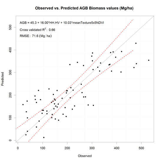
| Inputs for Tests | Selected via Stepwise Criteria | R2 LOO | RMSE LOO (Mg/ha) | R2 10-Fold | RMSE 10-Fold (Mg/ha) |
|---|---|---|---|---|---|
| (a). SAR HH and HV various statistics | HH + HV | 0.59 | 78.76 (0.15%) | 0.59 | 78.33 (0.15%) |
| (b). SAR HH and HV various statistics + GLCM HH and HV textures | HH + HV 5 × 5 HHmean | 0.65 | 71.95 (0.14%) | 0.65 | 72.09 (0.14%) |
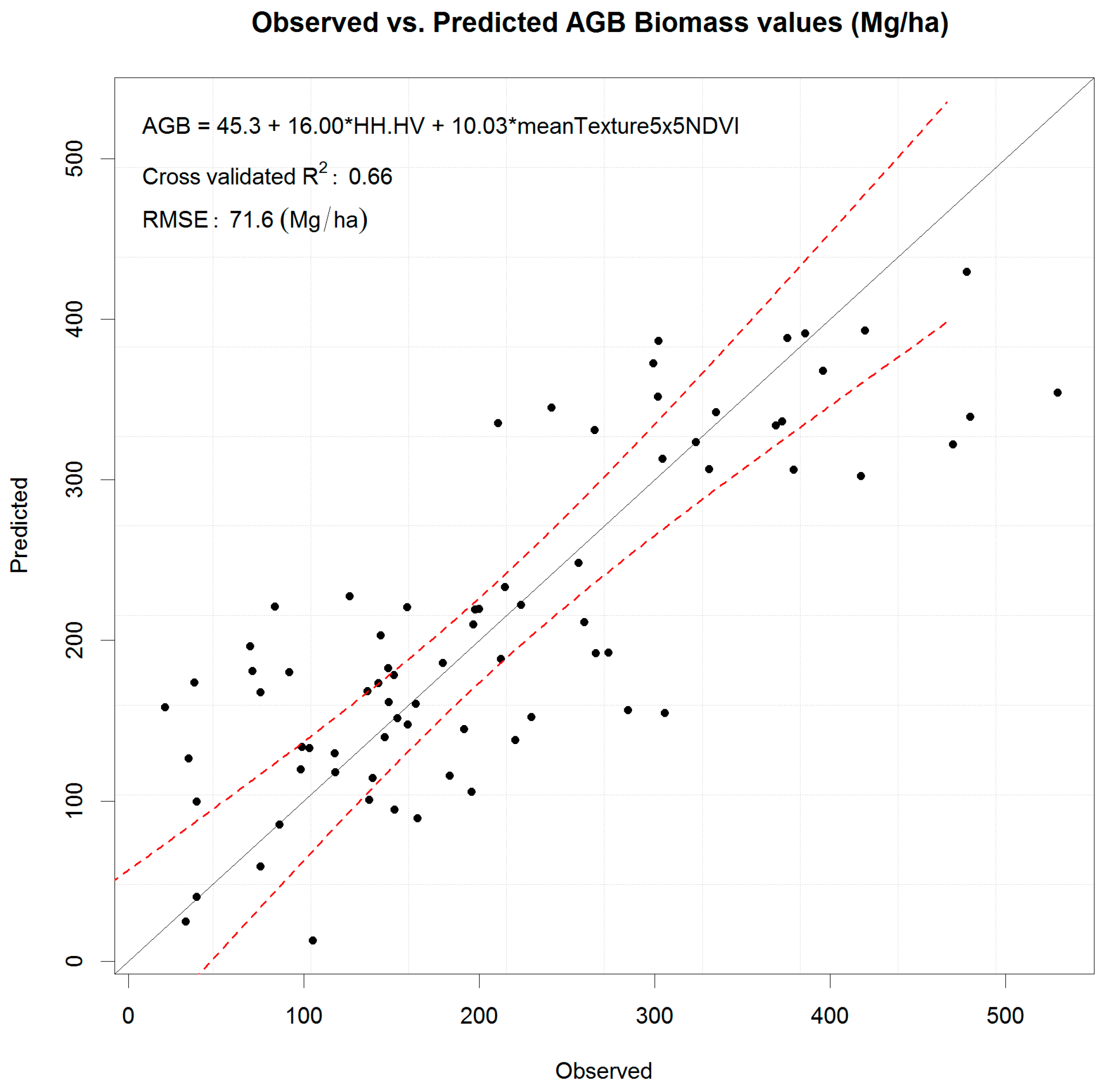
| (c). SAR HH and HV various statistics + NDVI + GLCM NDVI textures | HH + HV 5 × 5 NDVImean | 0.66 | 71.62 (0.14%) | 0.66 | 71.59 (0.14%) |
| (d). SAR HH and HV various statistics + 5 × 5 HHmean + 5 × 5 NDVImean | HH + HV 5 × 5 NDVImean | 0.66 | 71.62 (0.14%) | 0.66 | 71.59 (0.14%) |
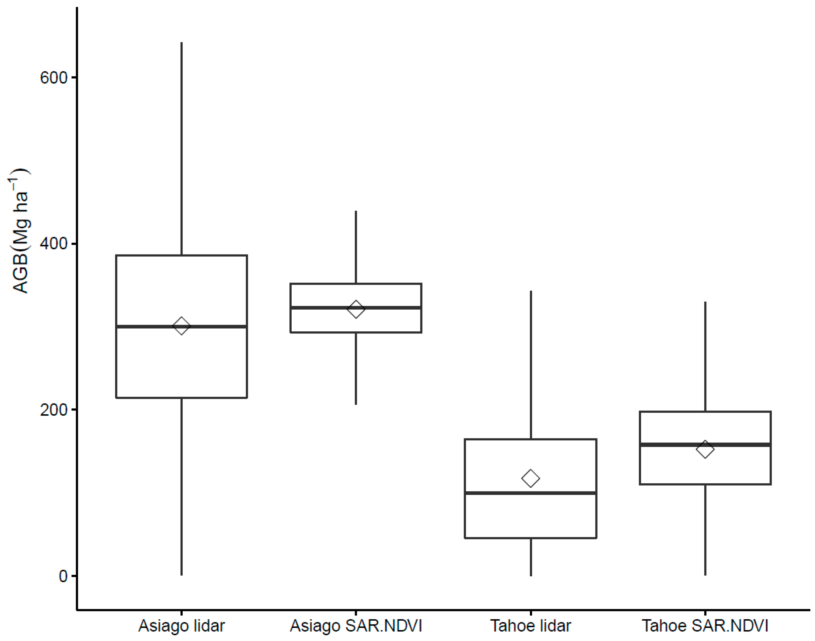
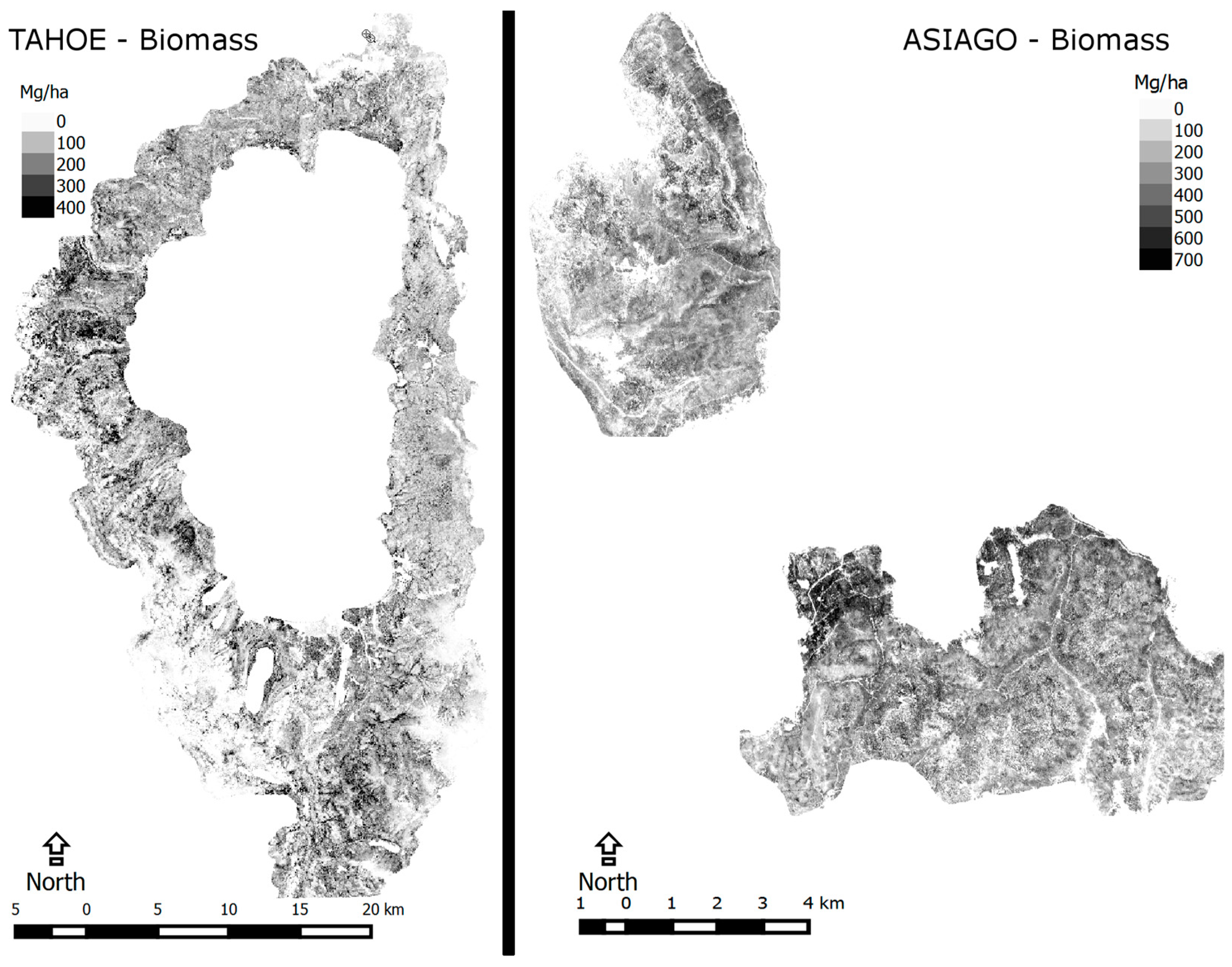
| Asiago SAR + NDVI | Asiago Lidar | Tahoe SAR + NDVI | Tahoe Lidar | |
|---|---|---|---|---|
| Mean AGB (Mg/ha) | 321 | 301 | 153 | 117 |
| Standard deviation of AGB (Mg/ha) | 49 | 117 | 64 | 94 |
| Total AGB (Mg) | 1.67 × 10⁶ | 1.57 × 10⁶ | 1.20 × 10⁷ | 0.97 × 10⁷ |
© 2016 by the authors; licensee MDPI, Basel, Switzerland. This article is an open access article distributed under the terms and conditions of the Creative Commons Attribution (CC-BY) license (http://creativecommons.org/licenses/by/4.0/).
Share and Cite
Vaglio Laurin, G.; Pirotti, F.; Callegari, M.; Chen, Q.; Cuozzo, G.; Lingua, E.; Notarnicola, C.; Papale, D. Potential of ALOS2 and NDVI to Estimate Forest Above-Ground Biomass, and Comparison with Lidar-Derived Estimates. Remote Sens. 2017, 9, 18. https://doi.org/10.3390/rs9010018
Vaglio Laurin G, Pirotti F, Callegari M, Chen Q, Cuozzo G, Lingua E, Notarnicola C, Papale D. Potential of ALOS2 and NDVI to Estimate Forest Above-Ground Biomass, and Comparison with Lidar-Derived Estimates. Remote Sensing. 2017; 9(1):18. https://doi.org/10.3390/rs9010018
Chicago/Turabian StyleVaglio Laurin, Gaia, Francesco Pirotti, Mattia Callegari, Qi Chen, Giovanni Cuozzo, Emanuele Lingua, Claudia Notarnicola, and Dario Papale. 2017. "Potential of ALOS2 and NDVI to Estimate Forest Above-Ground Biomass, and Comparison with Lidar-Derived Estimates" Remote Sensing 9, no. 1: 18. https://doi.org/10.3390/rs9010018
APA StyleVaglio Laurin, G., Pirotti, F., Callegari, M., Chen, Q., Cuozzo, G., Lingua, E., Notarnicola, C., & Papale, D. (2017). Potential of ALOS2 and NDVI to Estimate Forest Above-Ground Biomass, and Comparison with Lidar-Derived Estimates. Remote Sensing, 9(1), 18. https://doi.org/10.3390/rs9010018