Assessment of Carbon Flux and Soil Moisture in Wetlands Applying Sentinel-1 Data

Abstract

The objectives of the study were to determine the spatial rate of CO₂ flux (Net Ecosystem Exchange) and soil moisture in a wetland ecosystem applying Sentinel-1 IW (Interferometric Wide) data of VH (Vertical Transmit/Horizontal Receive—cross polarization) and VV (Vertical Transmit/Vertical Receive—like polarization) polarization. In-situ measurements of carbon flux, soil moisture, and LAI (Leaf Area Index) were carried out over the Biebrza Wetland in north-eastern Poland. The impact of soil moisture and LAI on backscattering coefficient (σ°) calculated from Sentinel-1 data showed that LAI dominates the influence on σ° when soil moisture is low. The models for soil moisture have been derived for wetland vegetation habitat types applying VH polarization (R² = 0.70 to 0.76). The vegetation habitats: reeds, sedge-moss, sedges, grass-herbs, and grass were classified using combined one Landsat 8 OLI (Operational Land Imager) and three TerraSAR-X (TSX) ScanSAR VV data. The model for the assessment of Net Ecosystem Exchange (NEE) has been developed based on the assumption that soil moisture and biomass represented by LAI have an influence on it. The σ° VH and σ° VV describe soil moisture and LAI, and have been the input to the NEE model. The model, created for classified habitats, is as follows: NEE = f (σ° Sentinel-1 VH, σ° Sentinel-1 VV). Reasonably good predictions of NEE have been achieved for classified habitats (R² = 0.51 to 0.58). The developed model has been used for mapping spatial and temporal distribution of NEE over Biebrza wetland habitat types. Eventually, emissions of CO₂ to the atmosphere (NEE positive) has been noted when soil moisture (SM) and biomass were low. This study demonstrates the importance of the capability of Sentinel-1 microwave data to calculate soil moisture and estimate NEE with all-weather acquisition conditions, offering an important advantage for frequent wetlands monitoring.

1. Introduction

Wetlands are very sensitive ecosystems, functioning as a habitat for many unique plants and animals. Wetlands play a significant role in many ecological functions including: carbon balance, regulation of the hydrological cycle, flood control, and the improvement and maintenance of water quality [1]. These areas remove atmospheric CO₂ through sequestration and subsequent peat accumulation, which can help to mitigate climate change effects. Those climate variations may also provide a significant influence on wetlands’ role in the carbon cycle by shifting from a sink to a sources mode of CO₂ [2]. The world’s peatlands cover only 5%–8% of the Earth’s land surface but store more organic carbon than any other terrestrial ecosystem i.e., an average of 118 g·C·m⁻²·year⁻¹ [3]. Many wetlands have been degraded by extraction for fuel, drainage, burning, overgrazing, urbanization, and atmospheric pollution. Degraded wetlands contribute 6% of global anthropogenic CO₂ [4], which could have an impact on climate change. Returning these ecosystems to a pre-anthropogenic-disturbance state by restoration is very important and can be treated as a buffer between the agricultural land and the surface water system (nutrient retention).

The Net Ecosystem Exchange (NEE) of CO₂ between the terrestrial ecosystem and the atmosphere reflects the balance between gross CO₂ assimilation (gross primary production—GPP) and ecosystem respiration (RESP). In it, photosynthesis processes are CO₂ sinks, and respiration processes are CO₂ sources. The NEE level is commonly measured by ground-based techniques such as Eddy Covariance [5,6,7,8,9,10,11,12,13,14,15,16] and chamber [17,18,19] methods. Remote sensing methods offer possibilities to evaluate NEE spatially, most often globally [20,21,22,23]. Wetlands are regarded as one of the difficult areas to monitor through conventional methods due to their relative inaccessibility and sensitivity to weather conditions. In-situ measurements are expensive and capable of providing data to a single, small area, and are difficult to use for mapping spatial variations. Microwaves can penetrate through vegetation and into soil, and thus can be widely used for the assessment of biomass and soil moisture [24,25,26,27,28,29,30] which are considered to have an impact on CO₂ flux. The relationship between microwave signal and soil moisture is complex as it depends on radar frequency, incidence angle, polarization, surface roughness and vegetation cover. For C band data, many studies showed that it is possible to estimate soil moisture with reasonably high accuracy [25,26,27,28,30,31]. Many of them concerned bare soils and agricultural areas [25,27,31]. Baghdadi et al [32] studied the application of RADARSAT-2 and LANDSAT-7/8 images to investigate the potential for the combined use of Sentinel-1 and LANDSAT-8 and Sentinel-2 data for soil moisture and Leaf Area Index (LAI) retrieval over irrigated grasslands. The results showed that HH (Horizontal Transmit/Horizontal Receive—like polarization) polarization is the most relevant to soil moisture estimates. Ulaby et al. [33] stated, that the sensitivity of microwave signals to soil moisture increases with a smaller incidence angle which allows better penetration of the wave. Also, the polarization of VV (Vertical Transmit/Vertical Receive—like polarization) has a higher penetration depth than HH. Zribi et al. [34] proposed the conventional empirical linear relationship approach between backscattering coefficient (σ°) calculated from ENVISAT-ASAR (ESA’s Environmental Satellite-Advanced Synthetic Aperture Radar) data registered in HH polarization with a dual-angle configuration and surface soil moisture of a small watershed. However, it can also be applied to vertical (VV) polarisation. Paloscia et al. [35,36,37] presented statistical algorithms for the retrieval of soil moisture over agricultural areas applying σ° in HH and HV (Horizontal Transmit/Vertical Receive—cross polarisation) polarizations from ENVISAT-ASAR data based on the Integral Equation Model (IEM) and the artificial neural network (ANN). Balenzano et al. [38] studied the potential of multi-temporal C- and L-band SAR data to map temporal changes of surface soil moisture. They found that low incidence angles (e.g., 20°–35°) and HH polarization are generally better suited to soil moisture retrieval underneath agricultural crops than VV polarization and higher incidence angles. Mattia et al. [39] investigated the radar sensitivity to biophysical parameters at different polarizations and incidence angles, and at different wheat phenological stages the experimental results, allowed to retrieve wheat biomass and soil moisture using Advanced Synthetic Aperture Radar data.

The aim of the study was to determine the spatial rate of CO₂ flux and soil moisture within a wetland ecosystem by applying soil-vegetation parameters represented by Sentinel-1 VH (Vertical Transmit/Horizontal Receive—cross polarization) and VV data. The work focused on:

• Classification of the wetland vegetation habitat types based on optical and microwave satellite images.
• Developing models for soil moisture assessment applying σ° calculated from Sentinel-1 data.
• Examination of influence of LAI and soil moisture on σ° calculated from Sentinel-1 data.
• Developing NEE models applying σ° calculated from Sentinel-1 VH and VV data.
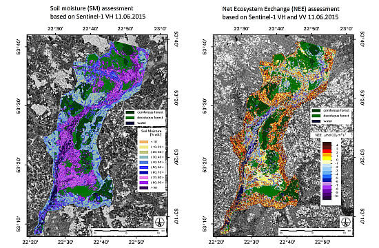
• Mapping spatial distribution of NEE over a test site area.

The investigation was carried out over the Biebrza Wetland located in North-East Poland from April to October in 2013–2015. For the year 2013 in-situ data for the classification of vegetation habitats have been carried out, and for the years 2014–2015 ground measurements of soil-vegetation parameters and carbon fluxes were done.

2. Materials and Methods

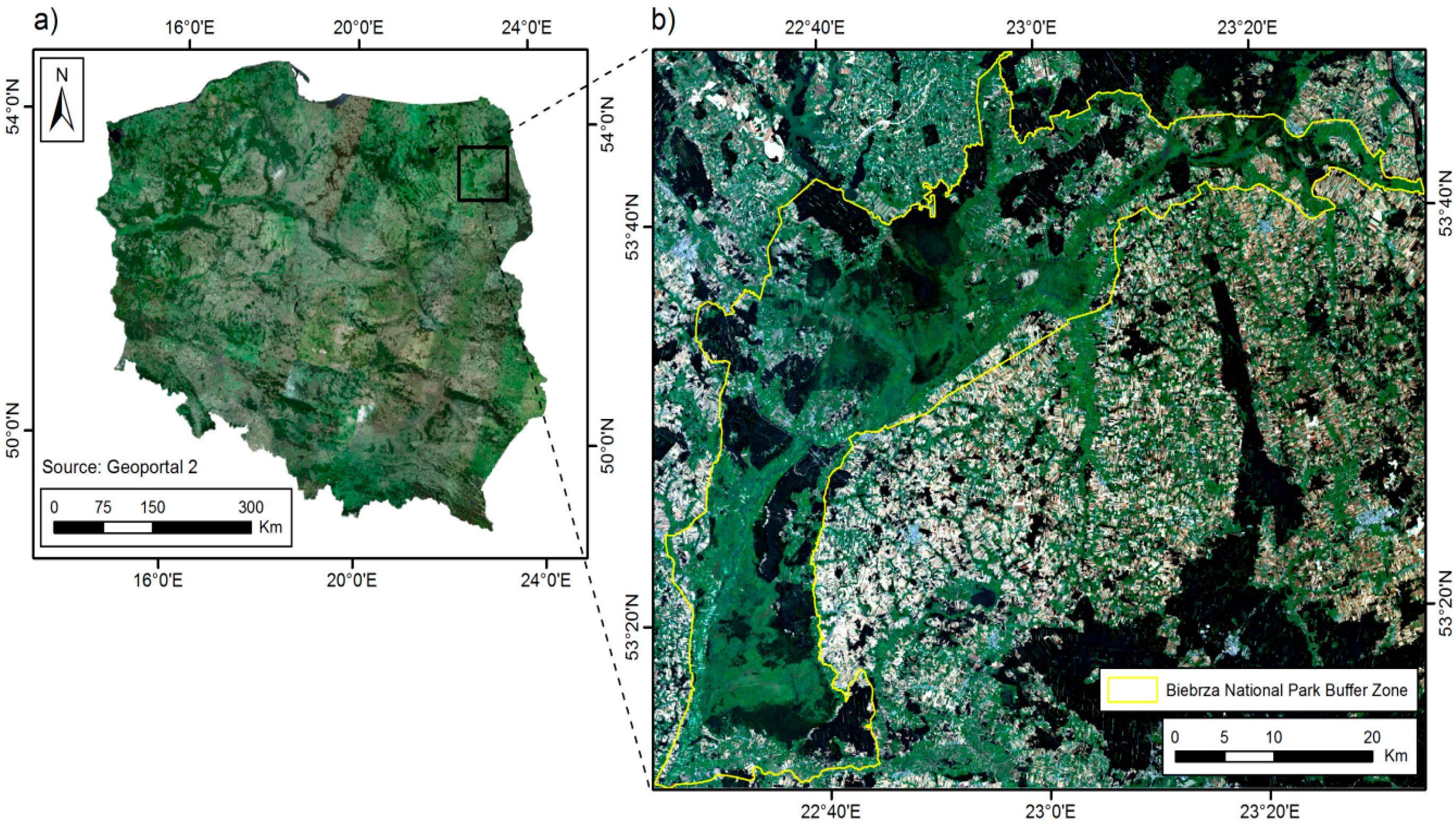
2.1. Test Site

The study was carried out at Biebrza Wetland test site, which is located in North-East Poland (UL coordinates: 53°50′′N, 22°10′′E; LR coordinates: 53°05′′N, 23°10′′E). Figure 1 presents the localization of the test site in Poland on the orthophotomap (Figure 1a) and the Biebrza Wetland area on Landsat 8 OLI (Operational Land Imager) RGB (Red, Green, Blue spectral bands 4,3,2) image registered on 3 August 2014 (Figure 1b). The Biebrza Wetland was designated as a wetland site of international importance in the NATURA 2000 Network and since 1995 has been under the protection of the RAMSAR Convention on Wetlands. The test site contains Biebrza National Park (BNP) established in 1993 with a total area of 59.233 ha which includes 15.547 ha of forests, 18.182 ha of agricultural land, and 25.494 ha of wetlands—the most valuable habitats of the park. It is a flat area with an average altitude of about 105 m above sea level, situated close to the Belarus border. The main river is Biebrza, which flows out near the eastern border of Poland and whose recipient is the Narew River.

The soils are mainly hydrogenic, with a dominant majority of peat soils in various stages of mouldering. The peatland complex covers about 90.000 ha and is the largest and the least disturbed of its kind in Central Europe. Wetlands floods occur annually in the spring and, besides precipitation, are the main supply of moisture into the peat soil. The site is characterized by large homogeneous fields of the following non-forest habitats: reeds, sedges, sedge-moss, grass, grass-herbs.

The weather is the coldest in Poland, with long winters (up to 120 days below zero) and a short growing season. The length of the summer ranges from 77 to 85 days, with daytime temperatures averaging 15 °C. The level of precipitation is one of the lowest in Poland—around 510 mm. The dry year was 2015, and normal years were 2013 and 2014.

2.2. Data Sets

The datasets used for the study were: in-situ measurements, TerraSAR-X (TSX) and Landsat 8 OLI images used for vegetation habitat types classification, and Sentinel-1 (S1) data used for examining the relationship of backscatter to soil moisture, LAI, and NEE.

Table 1. Microwave data acquisitions over the Biebrza Wetland test site.

Platform Sensor Mode	Band (cm)	Acquisition Date	Processing Level/Type	ENL 1	Beam Track	Spatial Resolution (m)	Polarization
TerraSAR-X SAR ScanSAR	X 3.1	21 May 2013	L1B GEC 2	1	scan_008	18	VV
		7 June 2013			scan_003
		23 June 2013			scan_008
Sentinel-1 SAR IW	C 5.55	31 October 2014	L1 GRD 3	5	29	10	VV/VH
		11 May 2015			29
		11 June 2015			131
		28 June 2015			29
		10 July 2015			29
		29 July 2015			131
		15 August 2015			29
		27 August 2015			29
		20 September 2015			29

¹ Effective Number of Looks; ² Geocoded Ellipsoid Corrected; ³ Ground Range Detected.

presents the list of microwave satellite data taken into the research: TerraSAR-X (X-band, wavelength 31 mm, frequency 9.65 GHz, ENL-1 (Effective Number of Looks), and Sentinel-1 (C-band, wavelength 5.55 cm, frequency 5.405 GHz, ENL-5).

TerraSAR-X images were registered in ScanSAR imaging mode and single polarization—VV. The TSX acquired product type was Geocoded Ellipsoid Corrected (GEC) in UTM projection. Sentinel-1 images were registered in Interferometric Wide (IW) mode, incidence angle 35° and dual polarization—VV and VH. The S1 acquired product type was Ground Range Detected (GRD) in WGS84 ellipsoid. The optical data—Landsat 8 OLI (Operational Land Imager) image registered on 19 May 2013 was applied in combination with TSX images in the classification procedure. This image was registered in nine spectral bands from 0.43 to 1.38 μm with a spatial resolution of 30 m for Bands 1 to 7 and 9, and 15 m for Band 8—panchromatic.

The in-situ measurements have been done from April to October of the years 2013–2015 at nearly 25 points distributed in various sites of the Biebrza Wetland in order to assess the distribution of soil moisture, vegetation parameters, and CO₂ flux over various types of vegetation habitats. During the field campaigns, each of the sites was treated three times in three different localizations around a measurement point for the calculation of the mean value. The dates of in-situ measurements corresponded to the dates of Sentinel-1 overpasses. The positions of the measurement plots were determined using GPS. Instantaneous flow of CO₂ between the ground surface and the atmosphere was measured using a static chamber method [40]. The concentration of CO₂ (ppm) and air temperature (°C) inside the plastic transparent chamber (40 × 40 × 35 cm) was measured by a portable non-dispersive infrared sensor (SenseAir^®, SenseAir SE) in one minute intervals. With this set-up, carbon flux (NEE) was first measured under light conditions immediately followed by a measurement of ecosystem respiration (RESP) after darkening of the chamber. The ground measurements also involved simultaneously measured significant vegetation and soil parameters such as: soil moisture in the layer of 0–15 cm (there is strong relationship between 0–5 cm and 0–15 cm for the peat soil) using the TDR method (TRIME-FM, IMKO Micromodultechnik GmbH, Ettlingen, Germany), LAI (LAI 2000, LiCor Inc., Lincoln, NE, USA), wet and dry biomass (in the laboratory from samples harvested inside the whole surface covered by the chamber following the flux measurement). All in-situ and satellite data have been stored in ACCESS and EXCEL databases.

2.3. Methods

The positions of the measurement plots, has been determined by GPS and were further used for preparing the measurement points layer which was needed for extracting satellite data.

Sentinel-1 IW and TSX ScanSAR microwave images have been processed using ESA Sentinel-1 Toolbox (S1TBX, developed for ESA by Array Systems Computing—Toronto, ON, Canada, in partnership with DLR—National Aeronautics and Space Research Centre, Germany, Brockmann Consult—Hamburg, Germany, and OceanDataLab—Locmaria Plouzane, France) in SNAP (Sentinel Application Platform, and is a common architecture for all Sentinel Toolboxes being jointly developed by Brockmann Consult and Array Systems Computing) to derive a backscatter coefficient (σ°) (dB). The processing included: speckle filtering applying Gamma-MAP filter 7 × 7, radiometric calibration and data conversion to backscattering coefficient. Then, scenes were geometrically registered to local projection PUWG1992 and S1 σ° values which corresponded to measurement points were extracted (5 × 5 pixels—within this area three in-situ measurements have been carried out to calculate mean value) using ERDAS software (Hexagon Geospatial/Intergraph^®, Norcross, GA, USA). Landsat 8 OLI images have been processed using ERDAS software. Then, the scene acquired in UTM map projection and WGS84 ellipsoid was geometrically registered to local projection PUWG1992. Atmospheric Correction of TOA reflectance (Top of Atmosphere) was not applied. It was not necessary for the classification process, which uses only one cloud-free image, as the training data and the data to be classified are in the same relative scale. [41].

The wetland vegetation habitats have been classified using combined one Landsat 8 OLI image and three TerraSAR-X ScanSAR VV images, all registered in the year 2013. These images have been chosen for classification, because of their high spatial resolution and the period of the growing season (before the first cut). Moreover, X-wave is dedicated to vegetation studies. Also, there was no possibility to acquire adequate optical and Sentinel-1 images for the study period. Landsat 8 OLI spectral bands have been resampled to pixel size of TSX images i.e., 18 m. The pixel-based supervised maximum likelihood classification method was applied using the ERDAS software. This type of classification has been used due to availability of adequate ground truth data collected in 2013 during field campaigns. The representative, homogeneous ground reference data were used for training and testing purposes. There were no changes in wetland vegetation type and cover from 2013 to 2015.

The collected time series of CO₂ flux concentration were validated in terms of temporal linearity. Fluxes with a correlation coefficient of the slope R² > 0.95 were accepted for further analysis. The CO₂ flux rate (NEE and RESP) was then calculated using the following equation described by Mosier and Mack in [42]:

$$\mathrm{E} =\mathsf{\rho }·\frac{\mathrm{V}}{\mathrm{A}}·\frac{\mathsf{\Delta }\mathrm{C}}{\mathsf{\Delta }\mathrm{t}}·\frac{273}{\mathrm{T}+273}$$

(1)

where: $\mathrm{E}$—CO₂ flux rate (mg m⁻²·h⁻¹); $\mathrm{V}$—chamber volume (0.056 m³); $\mathrm{A}$—collar area (m²); $\frac{\mathsf{\Delta }\mathrm{C}}{\mathsf{\Delta }\mathrm{t}}$—average rate of CO₂ concentration change with time; $\mathrm{T}$—air temperature in chamber (°C). NEE and RESP values were then predicted to μmol CO₂ m⁻²·s⁻¹ assuming that 1 μmol CO₂ weights 44 μg.

In-situ measured soil-vegetation parameters and satellite microwave data were analysed for wetland vegetation habitats. Simple and multiple regression analyses were used to create the best models—first to examine the relationship between soil moisture and the backscattering coefficient of Sentinel-1, as well as the relationship between LAI and σ° of S1. Data were checked for normal distribution and significance prior to all analysis. Statistical analyses for modeling NEE applying Sentinel-1 VV and VH data were done in STATISTICA and EXCEL software.

3. Results

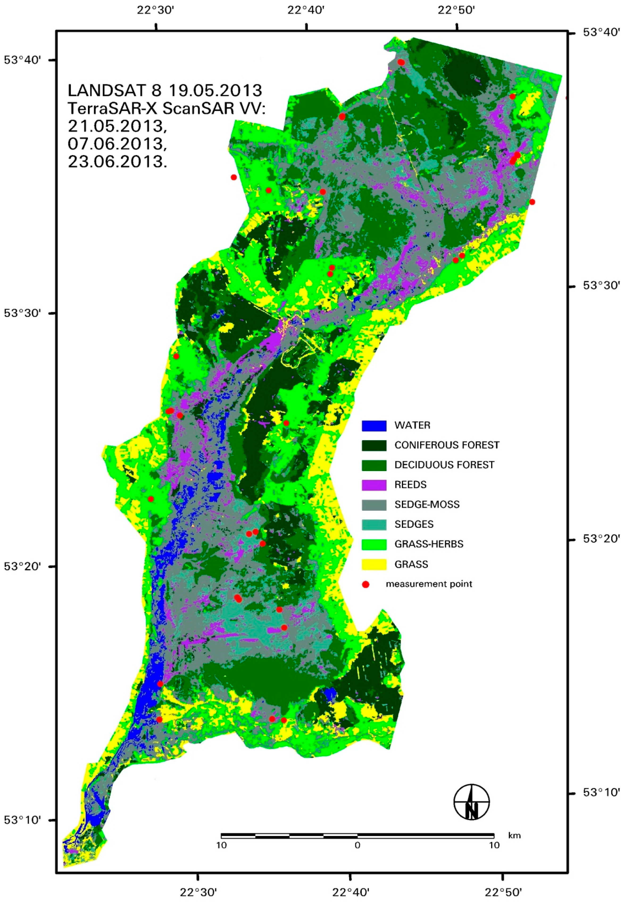
3.1. Classification of Wetland Vegetation Habitats

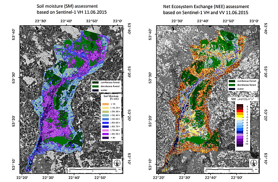
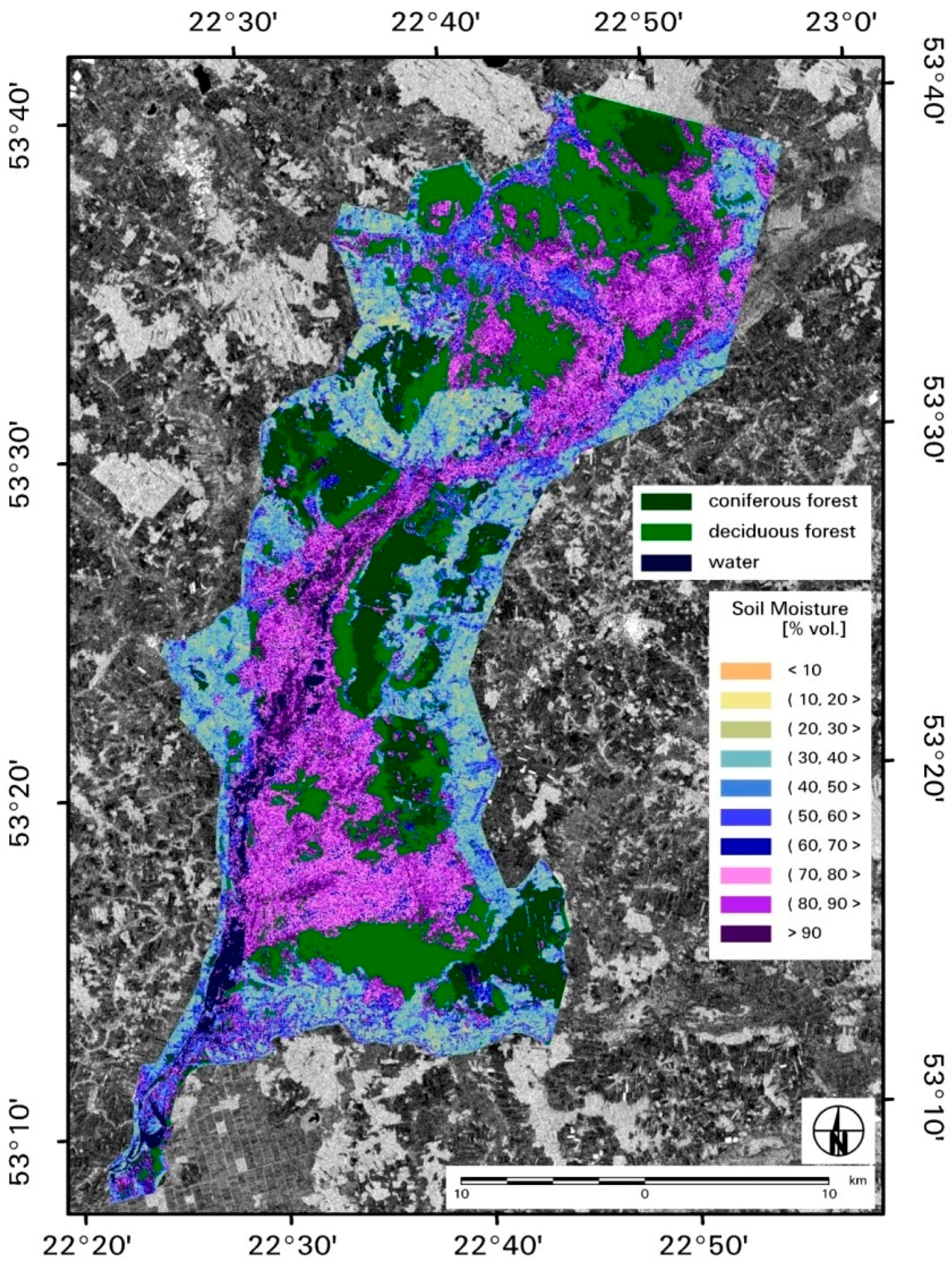
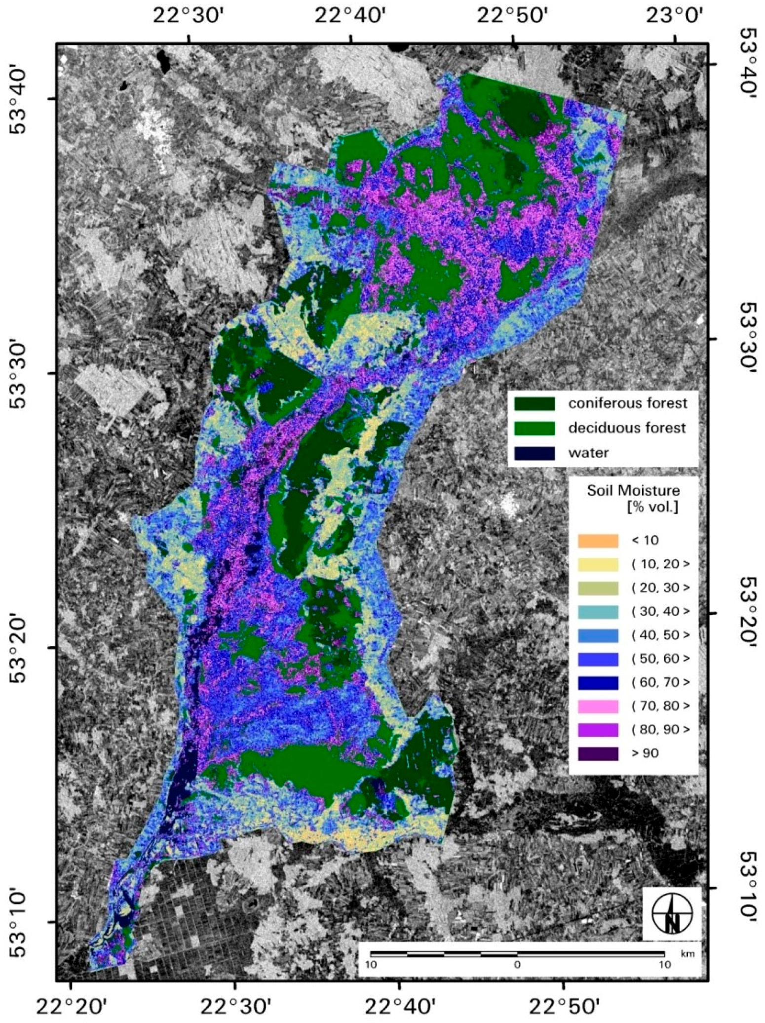
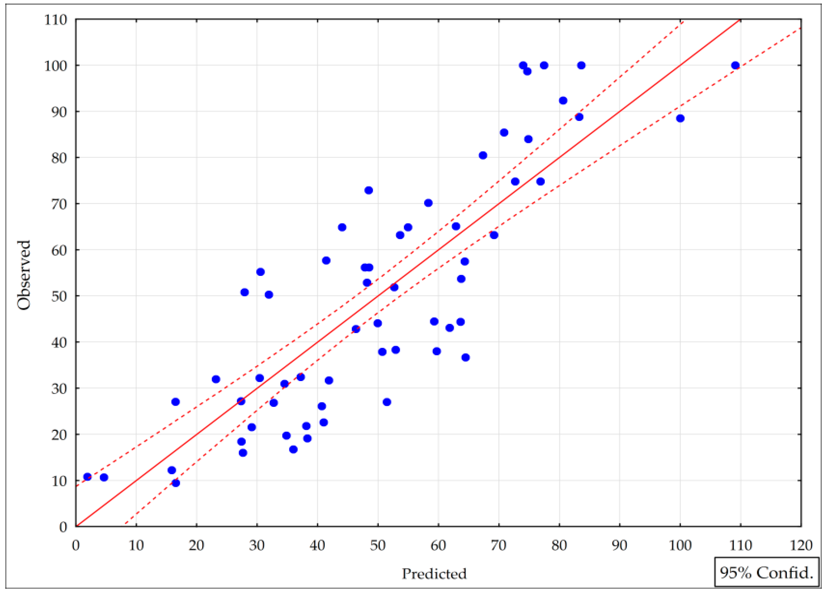
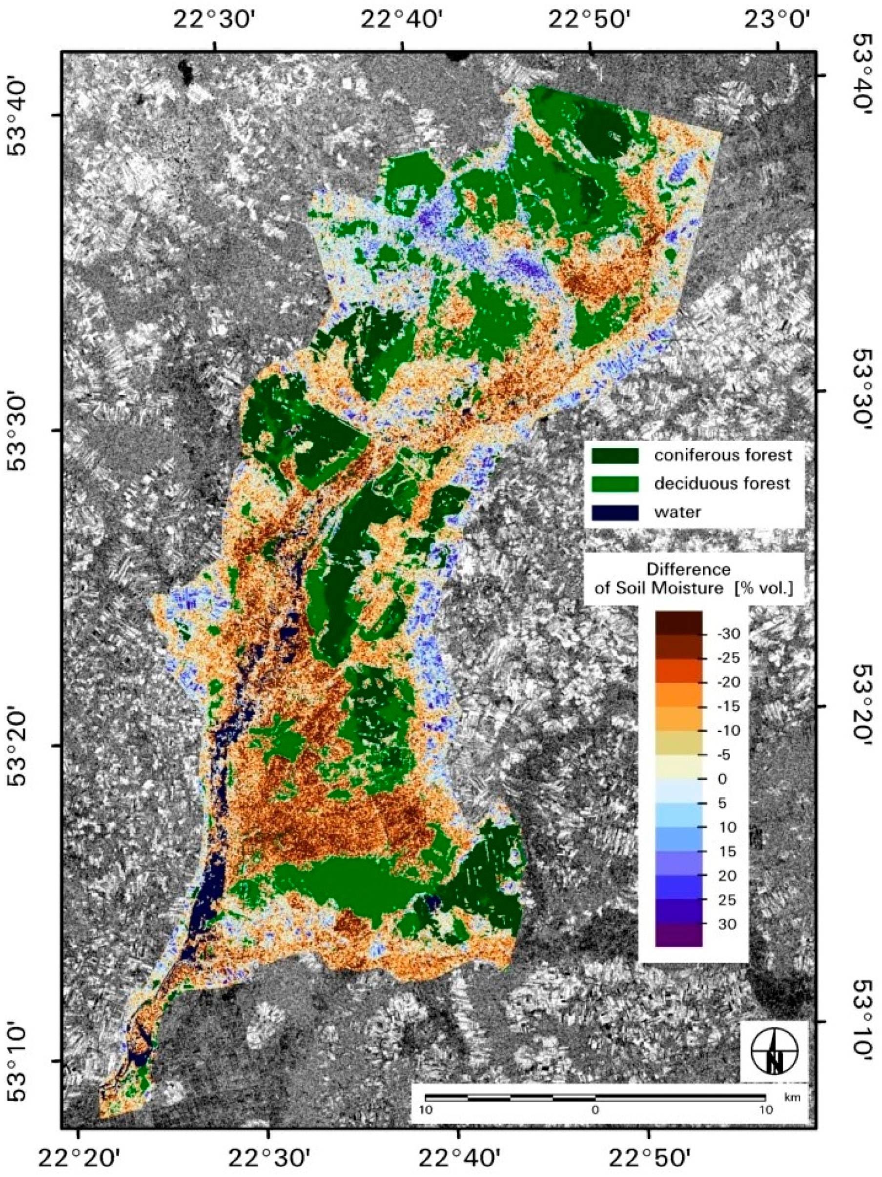
To estimate the relationship between microwave satellite data and soil-vegetation parameters precisely, there is a need to perform a classification of wetland habitats, as the relationships vary by the vegetation type. For the classification procedure, the following Landsat 8 OLI channels acquired on 19 May 2013 were chosen: 2 (0.45–0.51), 3 (0.53–0.59 μm), 4 (0.64–0.67 μm), 5 (0.85–0.88 μm), 6 (1.36–1.38 μm), and 7 (1.57–1.65 μm) along with three TerraSAR-X ScanSAR VV images acquired on 21 May 2013, 7 June 2013 and 23 June 2013. The validation and accuracy of the classification were performed using ground truth observations. As the results of wetland habitats classification, water and seven vegetation classes were distinguished: two forest habitats (coniferous and deciduous) and five representing most dominant non-forest wetland habitats: reeds, sedge-moss, sedges, grass-herbs, and grass.

Table 2. Error matrix for classified data in %.

Classified Data	Water	Coniferous Forest	Deciduous Forest	Sedge-Moss	Sedges	Grass-Herbs	Grass	Reeds
Water	99.67	0	0	0	0	0	0	0
Coniferous forest	0	99.28	0	0.28	0	0	0	0
Deciduous forest	0	0	99.51	0	0	0	0	0
Sedge-moss	0.33	0.5	0.3	92.13	8.23	0.63	0	3.58
Sedges	0	0	0.08	5.2	91.06	0	0	0.63
Grass-herbs	0	0.03	0.05	0.98	0.08	98.68	0	0
Grass	0	0	0.06	0.35	0.03	0.4	100	0
Reeds	0	0.19	0	1.05	0.6	0.29	0	96.79

presents the error matrix for classified data in %. The overall accuracy equals to 87.27% with 0.8333 of overall Kappa Statistics.

Table 3. Accuracy totals for each class.

Class Name	Reference Totals	Classified Totals	Number Correct	Producers Accuracy (%)	Users Accuracy (%)
Water	6	6	6	100	100
Coniferous forest	16	17	16	100	94.12
Deciduous forest	31	26	26	83.87	100
Sedge-moss	21	31	21	100	67.74
Sedges	12	8	8	66.67	100
Grass-herbs	14	15	12	85.71	80
Grass	10	9	9	90	100
Reeds	5	3	3	60	100

presents accuracy totals for each of the classes. Figure 2 presents a map of classified wetland habitat types.

3.2. Soil Moisture

In-situ soil moisture (SM) values (ranged from 10% to 100% volumetric.) from the test site have been related to the backscattering coefficient (σ°) calculated from Sentinel-1 IW VV and VH data, applying various regression models. The best results have been found applying VH polarization and a linear model performed for particular vegetation habitat types separately (Figure 2). These results are presented in

Table 4. Results of relationships at a 95% confidence level between measured soil moisture (SM) and σ° calculated from Sentinel-1A VH data.

Platform Sensor	Habitat	R2	St. Error of Est.	Number of Data	p-Value	Equation
Sentinel-1 IW VH	Reeds	0.71	14.35	29	0.0000	SM = 233.791 + 9.805 × σ°
	Sedge-moss	0.76	11.23	30	0.0000	SM = 278.537 + 11.898 × σ°
	Sedges	0.76	11.15	41	0.0000	SM = 218.194 + 8.586 × σ°
	Grass-herbs	0.70	7.01	33	0.0000	SM = 130.341 + 5.271 × σ°
	Grass	0.75	6.14	49	0.0000	SM = 136.539 + 5.253 × σ°

. The relationships between SM and σ° at the 95% confidence level is statistically significant (p < 0.05). The highest correlation belongs to σ° calculated from Sentinel-1 IW VH data for sedge-moss and sedges, the most typical wetland habitats. Slightly better results have been found applying an exponential model.

Derived equations (Table 4) were used to map soil moisture distribution over the Biebrza Wetland. Figure 3 and Figure 4 present two maps composed using Sentinel-1 VH data acquired on 11 June 2015 and 10 July 2015, respectively, as an example. It can be noted that much lower SM value in July compared to June was caused due to severe drought, which started in May.

Figure 5 and Figure 6 present relationships between soil moisture measured in-situ and calculated from Sentinel-1 IW VV and VH data (respectively) applying a statistically derived algorithm (

Table 5. Results of the relationships at the 95% confidence level between measured SM and calculated SM from Sentinel-1 VV and VH data.

Platform Sensor	Habitat	R2	Standard Error of Est.	Number of Data	p-Value	Equation
Sentinel-1 IW VV	all	0.63	15.28	58	0.0000	SM = 235.666 + 14.980 × σ°
Sentinel-1 IW VH	all	0.72	14.32	62	0.0000	SM = 347.273 + 15.413 × σ°

). The analyses were performed for all wetland habitats (for a representative sample). The coefficient of determination (R²) between SM and σ° VH is comparable to the R² obtained between SM and σ° VV. The R² are slightly lower from that obtained for particular habitat classes separately (Table 4). Table 5 presents results of these statistical analyses which could be applied for mapping soil moisture without the need for classification of the vegetation habitat types.

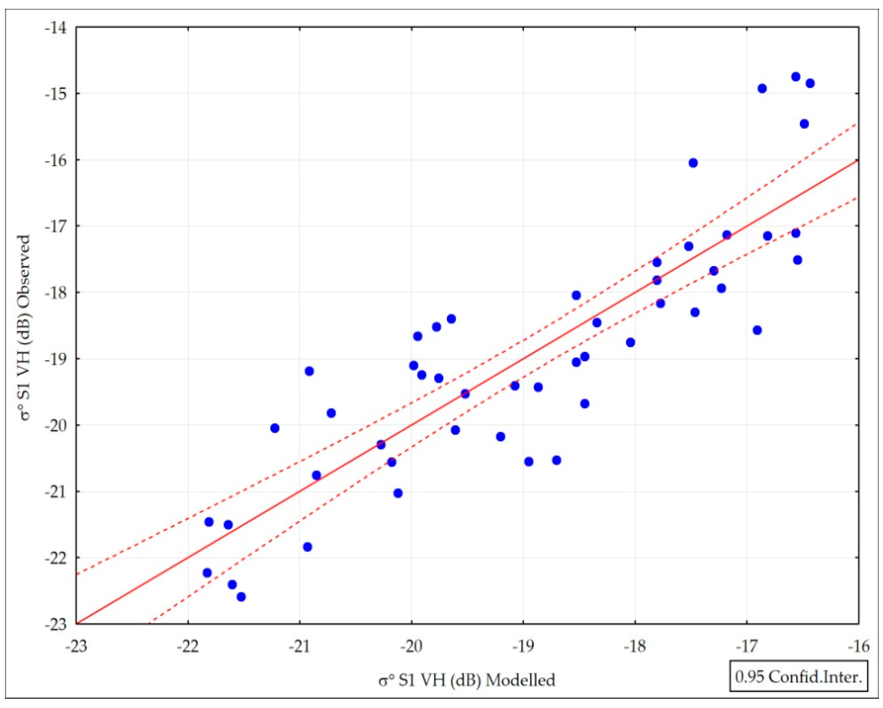
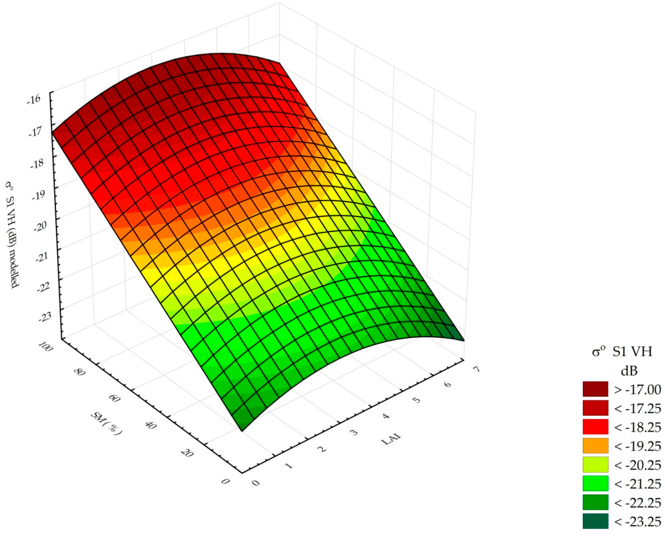
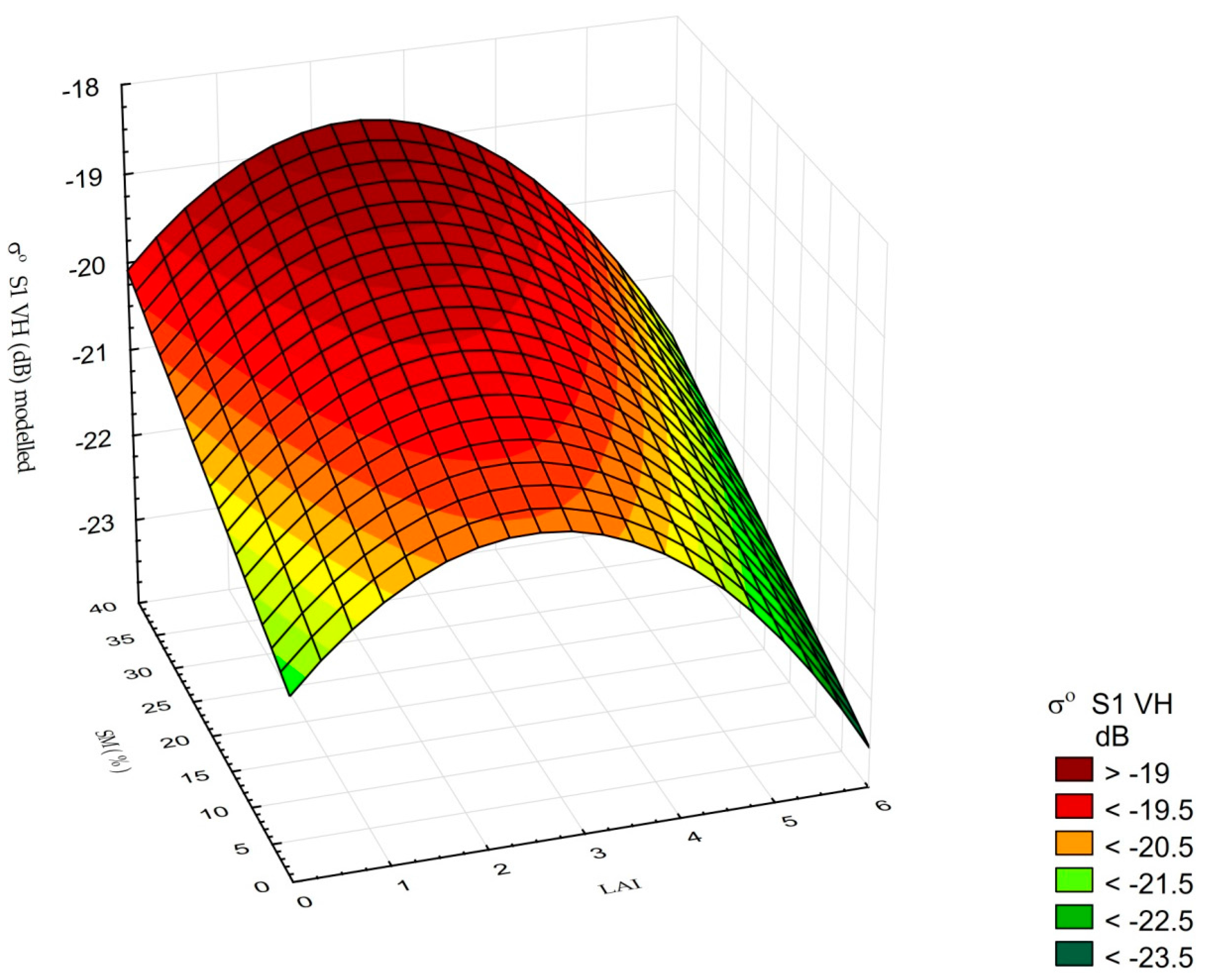
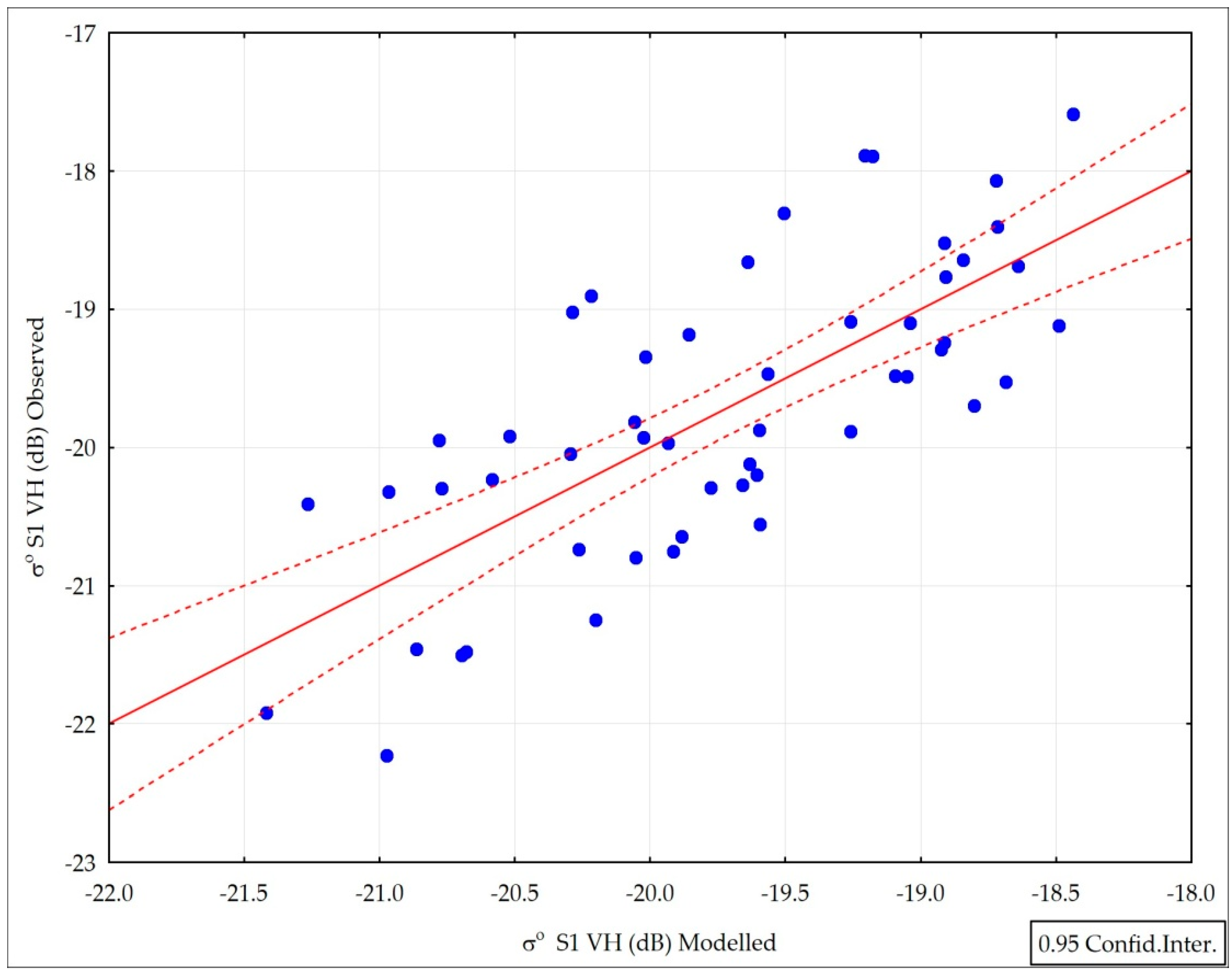
3.3. Influence of LAI and Soil Moisture on σ° Calculated from Sentinel-1 Data.

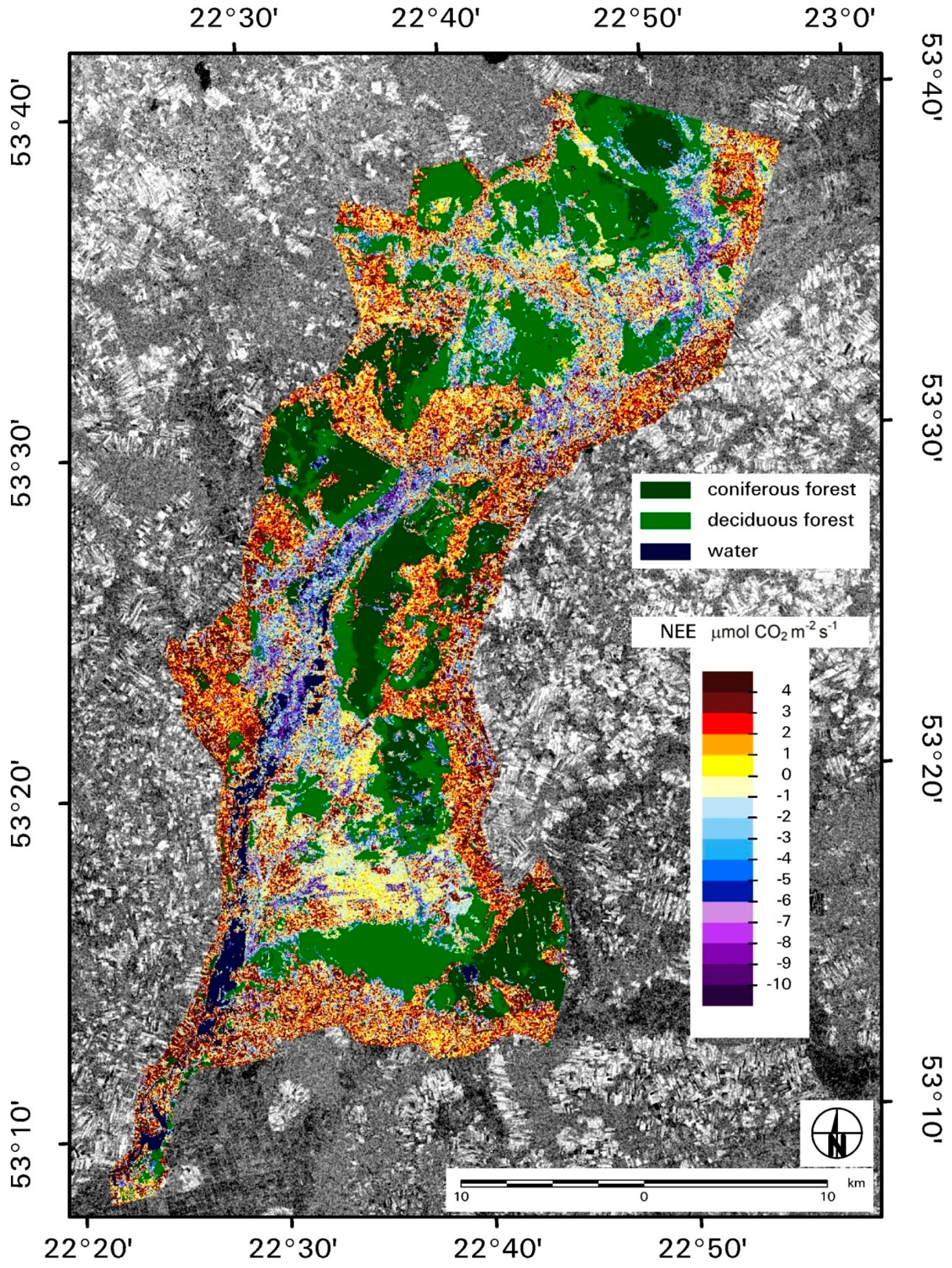
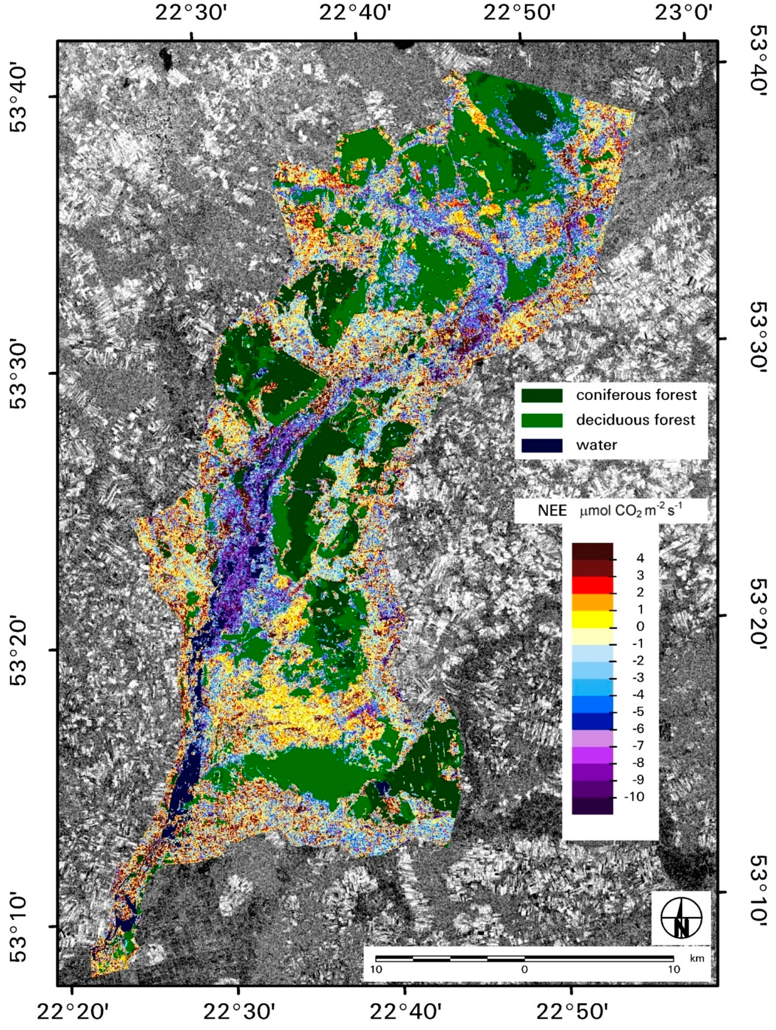
There is a relationship between leaf area index (LAI) and wet biomass (Bw) (both measured in-situ) independent of vegetation habitat types. Figure 7 presents the best fit which was a power model at a 95% confidence level. The data also include measurements taken from the previous studies. A large increase in R² was achieved when particular habitat types (Figure 2) were included in the analysis separately.

Table 6. Results of the relationships at the 95% confidence level between measured in-situ LAI and Bw.

Habitat	R2	St. Error of Est.	Number of Data	p-Value	Equation
Reeds	0.66	0.32	116	0.0000	LAI = 0.077Bw0.533
Sedge-moss	0.67	0.29	149	0.0000	LAI = 0.041Bw0.646
Sedges	0.70	0.36	112	0.0000	LAI = 0.023Bw0.722
Grass-herbs	0.67	0.37	214	0.0000	LAI = 0.016Bw0.787
Grass	0.69	0.34	207	0.0000	LAI = 0.022Bw0.749

presents results of statistical analyses performed for each of the classified non-forest wetland habitats. The highest R² has been found for sedges, the lowest for reeds, very often water logged.

LAI can be estimated by applying optical or microwave satellite data [31,43,44]. In the present study the analysis between LAI and the backscattering coefficient calculated from Sentinel-1A data has been investigated by means of regression models. Vegetation covering the soil plays a certain role on the registered microwave signal. In the present study, it has been examined how vegetation (represented by LAI) affects the S1 microwave signal. At fixed LAI values, soil moisture is in simple linear correlation with σ° VH, but otherwise the dependence of LAI on backscatter has a polynomial character. The linear multiply regression model of σ° VH includes these two components as the independent variables. The resulted regression equation was as follows:

σ° VH = −22.45 + 0.05 × SM + 0.55 × LAI − 0.086 × LAI²

(2)

where R² = 0.75, p < 0.05. Figure 8 presents the scatterplot of this model. The root mean square error (RMSE) and the mean bias error (MBE) were used as the model performance indicators for the training and validation datasets. The RMSE was equal to 0.89 dB and MBE was equal to 0.002 dB for the training dataset (49 points). RMSE was equal to 1.8 dB and MBE was equal to −0.37 dB for the test containing 63 observations.

The partial correlations for the particular components have been examined. For the model presented by Equation (2) the R was equal to 0.85 for SM, and for LAI—R was equal to 0.22 (expression of LAI in Equation (2) was treated as one component). It means that the influence of SM for the explanation of the variance of σ° VH, after establishing the influence of LAI, is several times stronger than the influence of LAI when SM is constant. Figure 9 illustrates this case in 3D space. A full range of soil moisture under fixed LAI caused the variation of σ° VH up to 5 dB. The case of LAI under fixed SM caused a variation of σ° VH of only 1.2 dB. It can be concluded that the influence of LAI on σ° is slightly over the statistical error (0.89 dB).

The influence of the two components, LAI and SM, on σ° VH values when the soil moisture is low was examined. The model described by Equation (3) presents the relationship of LAI and SM for the conditions when soil moisture was lower than 40%.

σ° VH = −11.6 + 0.046 × SM + 1.12 × LAI − 0.24 × LAI²

(3)

Figure 10 presents the relationship between observed and modelled σ° VH (dB) for SM <40, where R² = 0.6, p < 0.05, number of observations—52, RMSE = 0.73 dB, MBE = 0.1 dB. When LAI is constant, the partial correlation for SM explaining σ° VH variation gave R equal to 0.61, and R was equal to 0.48 for LAI explaining σ° VH variation when SM is constant.

With fixed low soil moisture values, the range of backscatter variance depended on LAI and could increase up to 3.2 dB. When LAI is on a fixed level, the variance of backscatter caused by SM gets up to 2.4 dB, (Figure 11). Contribution of LAI to backscatter VH was higher when SM values were low. High difference of σ° VH between two points covered by vegetation does not mean that the soil moisture is really different. In the model (3) σ° VH >−19 dB represents a high value of LAI for SM of about 30%–40%. The same values of σ° VH, i.e., >−19 dB in the model (2) occurred for high SM (>70%) independently of LAI (Figure 9 and Figure 11).

3.4. NEE Modeling

NEE values measured in-situ (Section 2.2) were related to various in-situ and satellite data to derive prediction models. The analyses were performed for particular vegetation habitat types (Figure 2) separately. The best models were found by applying Sentinel-1 to both VH and VV polarization (

Table 7. NEE (Net Ecosystem Exchange) models at 95% confidence level derived by applying in-situ and Sentinel-1 satellite data.

Platform Sensor	Habitat	R2	Standard Error of Est.	p-Value	Equation
Sentinel-1 IW VH VV	Reeds	0.57	2.75	0.0043	NEE = −42.85 − 4.25 × σ°S1VH + 2.71 × σ°S1VV
	Sedge-moss	0.58	2.02	0.0057	NEE = −7.22 + 1.42 × σ°S1VH − 2.74 × σ°S1VV
	Sedges	0.51	1.57	0.0024	NEE = −2.28 − 0.86 × σ°S1VH + 1.08 × σ°S1VV
	Grass-herbs	0.51	2.75	0.0072	NEE = 27.75 + 1.87 × σ°S1VH − 0.65 × σ°S1VV
	Grass	0.55	3.07	0.0001	NEE = 11.22 + 2.34 × σ°S1VH − 2.72 × σ°S1VV

). These were multiple linear regression models. Since the p-value was less than 0.05, there is a statistically significant relationship between the variables at the 95.0% confidence level. The R² indicates that the model explains no more than 51%–58% of the variability in NEE. Thus, these preliminary results have to be validated and the model has to be corrected to improve statistical correlation. Equations from Table 7 have been applied for the NEE mapping over the Biebrza Wetland. Figure 12 and Figure 13 present maps of NEE distribution over classified wetland habitats for two dates: 11 June 2015 and 10 July 2015. The NEE values varied from 4 to −10 μmol CO₂ m⁻²·s⁻¹. The prevailing NEE positive values (CO₂ emission to atmosphere, mean from 1 to 4 μmol CO₂ m⁻²·s⁻¹) at the date 11 June 2015 belong to grass, grass-herbs, and sedges habitats, the biomass values of which were low at that time (harvested or grazed). For the date 10 July 2015 CO₂ absorption dominated (NEE negative values, mean from −1 to −10 μmol CO₂ m⁻²·s⁻¹) in the most moist habitats, i.e., reeds and sedge-moss, while emission was noted for the lower soil moisture values (NEE values were positive, mean: 0–2 μmol CO₂ m⁻²·s⁻¹).

4. Discussion

4.1. Classification of Wetland Vegetation Habitat Types

Classification of wetland vegetation habitat types using remote sensing data has been undertaken many times. The methods, most often used, concerned the application of optical data [44,45,46,47,48]. Dabrowska-Zielinska et al. [44] derived six wetland habitats from the classification of MERIS (Medium Spectral Resolution Imaging Spectrometer) images acquired on 21 April 2003: anthropogenic, pastures, sedge-mursh, rush-sedge, reeds, and scrubs. Wright and Gallant [48] distinguished five classes: aquatic bed (vegetation on or below the water surface), emergent (herbaceous hydrophytes), forested, scrub-shrub (height < 6 m), and unconsolidated shore, applying Landsat TM imagery. Recently, the application of microwave data for the classification of vegetation habitats has been expanded by Evans et al. [49,50]. Santoro et al. [51] who studied ALOS PALSAR (Advanced Land Observing Satellite Phased Array type L-band Synthetic Aperture Radar) data found that better classification results were obtained from HV than from HH polarization. Dabrowska-Zielinska et al. [43] and Conforth et al. [52] also presented wetland classification using ALOS PALSAR data acquired in HV polarization. Flores De Santiago et al. [53] found that a combination of HH and HV polarization modes from ALOS PALSAR data was better at separating forested wetlands using an object-based classification approach. Bwangoy et al. [54] applied optical (Landsat TM (Thematic Mapper) and ETM+ (Enhanced Thematic Mapper Plus) and JERS-1 (Japanese Earth Resources Satellite-1) data to classify the wetland and non-wetland classes of the Congo Basin. Ozesmi and Bauer [55] reported that the combination of radar and optical data will improve wetland classification.

There is a lack of a detailed classification of European wetland vegetation. In this study we decided to apply microwave and optical data for the classification of wetland vegetation habitats. Compared to the classification results undertaken using ALOS PALSAR HV [43], in the present study it was possible to distinguish wetland habitat types more precisely. The obtained classification results of wetland habitat types (two forest and five non-forest habitats) presented in Figure 2 were not found in the literature before and are promising in wetland changes monitoring.

4.2. Soil Moisture

Soil moisture retrieval methods from single polarisation, active, spaceborne, microwave observations were described by Barrett et al. in [56]. Baghdadi et al. [57] applied ENVISAT ASAR data for soil moisture retrieval over bare soils. The research on application of radar data for soil moisture assessment has been published for inland wetlands at High Latitudes applying C-band SAR (Synthetic Aperture Radar) data—Reschke et al. in [58], Bartsch et al. in [59], and Kasischke et al. in [60]. They stated that C-band backscatter may be enhanced by inundation or high levels of soil moisture, what has been presented in our study. Paloscia et al. applied ENVISAT ASAR [35] and Sentinel-1 [61] images for soil moisture assessment over vegetated areas. Kornelsen and Coulibaly [62] conducted a comprehensive literature review of SAR soil moisture retrieval methodology, its limitations and potential. Hornáček et al. [63] presented the potential for surface soil moisture retrieval via the Change Detection method using Sentinel-1 data. Dorigo et al. [64] presented the evaluation of CCI (Climate Change Initiative) soil moisture product using ground based observations. Soil moisture for the Biebrza Wetland has been investigated by authors in a previous study using microwave data acquired by ERS-1/2 SAR VV, ENVISAT ASAR IS2 HH, and ALOS PALSAR HH [25,43,44,65,66]. In the present study Sentinel-1 IW VV and VH data have been applied for the assessment of soil moisture (there was no S1 acquisition in HH polarisation). The best results have been found applying VH polarization. In general, the results are consistent with the literature, however most of the research presented in the literature was done for other than wetlands areas. The models developed by the authors will be validated and corrected using S1 and in-situ data acquired in the year 2016.

For soil moisture change detection, the image differencing method was used. Differencing involved the subtraction of backscattering coefficient values between two different date images. Figure 14 presents a soil moisture difference map created by applying data from the dates: 10 July 2015 and 11 June 2015. The advantage of this technique is that, in cases where vegetation surface roughness doesn't change in time, the difference in backscatter between two dates can be related solely to a change in the soil moisture content. Soil moisture and vegetation represented by LAI were observed as having influence on the value of σ° calculated from Sentinel-1 VH data. Soil moisture is in simple correlation with σ°, but the dependence of LAI has a polynomial character. The dependence of LAI on backscatter is associated with low or high soil moisture. That’s why the research on the influence of soil moisture and vegetation cover should be continued under different soil-vegetation conditions.

4.3. Influence of LAI and Soil Moisture on σ° Calculated from Sentinel-1 Data.

The assessment of LAI using ENVISAT MERIS and ASAR data was presented by Dabrowska-Zielinska et al. in [44,62,63]. This was done for the wetland habitats distinguished from the classification of MERIS image. LAI prediction, applying ALOS PALSAR HV data, was presented by Dabrowska-Zielinska et al. in [43,65,66]. The obtained results showed that with the increase of LAI there was an increase in the backscattering coefficient, which indicates the low signal attenuation by vegetation in L-band, contrary to results obtained in C- and X-band. For LAI assessment, the ASAR mode with higher incidence angles gives better results, which have been examined by authors in other studies [67], applying VV IS6 data for the agriculture area. In the present study, the influence of LAI and SM on σ° calculated from Sentinel-1 data has been examined. Two linear multiply regression models of σ° VH that include these two components as the independent variables have been developed. Comparing the results of model (2) and model (3), it has to be noted that the influence of LAI on σ° VH value is much stronger when soil moisture values are low (<40%). The obtained results are promising and will be validated in the future work using new satellite and in-situ data.

4.4. NEE Modeling

The studies on carbon exchange in grassland areas applying in-situ and satellite MODIS (Moderate-Resolution Imaging Spectroradiometer) and TerraSAR-X StripMap VV data have been presented by authors in [68]. The results showed significant correlations between NEE and Normalised Difference Vegetation Index - NDVI (R² = 0.56), and between surface temperature (Ts) and RESP (R² = 0.54). Also, a significant relationship has been found between NEE and σ° calculated from TSX data (R² = 0.53)—the higher CO₂ absorption corresponded to higher NDVI and σ° values. The proposed model for Net Ecosystem Exchange is based on a simple relationship with Sentinel-1 VV and VH data, which are actually delivered with high temporal resolution. This gives the possibility of frequent monitoring of the wetlands ecosystem, especially important under high soil-vegetation dynamics. However, these preliminary results have to be validated and corrected to improve statistical correlation. The carbon flux depends mainly on vegetation and humidity conditions. The study explained why the microwave data of Sentinel-1 VH and VV give promising results to the NEE estimates. Changes in soil moisture and vegetation cover (cuts or grazing) of the wetlands vegetation causes the carbon balance disturbance. Since wetland ecosystems are very important in carbon cycling, they have to be monitored regularly, which is possible by applying Sentinel-1 data.

5. Conclusions

At the Biebrza wetland study site it has been demonstrated that:

(1)

Wetland vegetation habitats have been classified using a combination of one optical (i.e., Landsat 8 OLI) and three microwave (i.e., TerraSar-X VV) images. The remote sensing based classification distinguished several wetlands’ non-forest classes that have not been noticed before, which is novel.

(2)

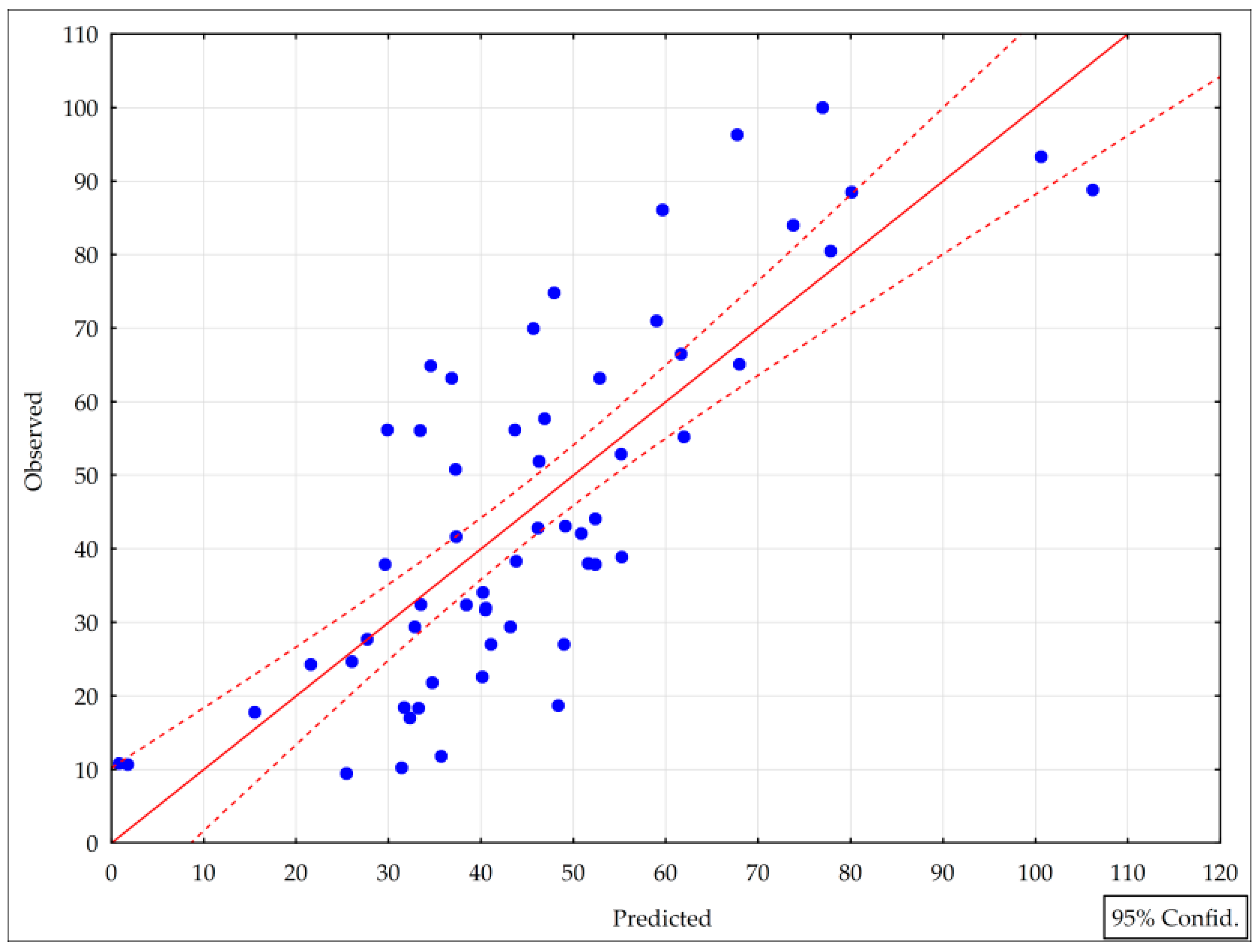
Soil moisture could be assessed using Sentinel-1 data acquired in VH polarisation. However, these preliminary results have to be validated and models corrected using new acquisitions. Also, if available in the future, S1 HH polarisation will be included for SM modelling.

(3)

There is the influence of soil moisture and vegetation biomass represented by LAI on σ° VH, however soil moisture impact on backscatter is stronger.

(4)

Comparing the results of model (2) and model (3), it has to be noted that the influence of LAI on σ° VH value is much stronger when soil moisture is low.

(5)

NEE in-situ measurements had positive values during dry soil conditions and low biomass means that CO₂ was released into the atmosphere. Also, when dry vegetation was over the water table in the flooded area, NEE values were positive. For the wet soil moisture conditions and high biomass, CO₂ absorption dominated (NEE negative values).

(6)

NEE could be assessed by applying combined Sentinel-1 VV and VH data. However, to obtain better accuracy, statistical correlation should be improved. These preliminary results will be validated and the model corrected by applying new satellite acquisitions and in-situ data.

The research has been done for wetlands where moisture of the peat soil cannot be compared to the moisture of mineral soils in agriculture areas. The peat soils were constantly covered by vegetation in the vegetation growth cycle. That’s why the study on the application of radar data for moisture variation of peatland is difficult and in a sense unique. The results of the study could be useful for the CCI soil moisture product presented by Dorigo et al. [64].

References

1. Mitsch, W.J.; Gosselink, J.G. Wetlands: Human History, Use, and Science. In Wetlands, 4th ed.; John Wiley & Sons Inc.: Hoboken, NJ, USA, 2007; pp. 3–5. [Google Scholar]
2. Wu, J.; Roulet, N.T. Climate change reduces the capacity of northern peatlands to absorb the atmospheric carbon dioxide: The different responses of bogs and fens. Glob. Biogeochem. Cycles 2014, 28, 1005–1024. [Google Scholar] [CrossRef]
3. Mitsch, W.J.; Bernal, B.; Nahlik, A.M.; Mander, U.; Zhang, L.; Anderson, C.J.; Jorgensen, S.E.; Brix, H. Wetlands, carbon, and climate change. Landsc. Ecol. 2013, 28, 583–597. [Google Scholar] [CrossRef]
4. Blundell, A.; Holden, J. Using palaeoecology to support blanket peatland management. Ecol. Indic. 2015, 49, 110–120. [Google Scholar] [CrossRef]
5. Mudge, P.L.; Wallace, D.F.; Rutledge, S.; Campbell, D.I.; Schipper, L.A.; Hosking, C.L. Carbon balance of an intensively grazed temperate pasture in two climatically contrasting years. Agric. Ecosyst. Environ. 2011, 144, 271–280. [Google Scholar] [CrossRef]
6. Acharya, B.R.; Rasmussen, J.; Eriksen, J. Grassland carbon sequestration and emissions following cultivation in a mixed crop rotation. Agric. Ecosyst. Environ. 2012, 153, 33–39. [Google Scholar] [CrossRef]
7. Felber, R.; Neftel, A.; Ammann, C. Discerning the cows from the pasture: Quantifying and partitioningthe NEE of a grazed pasture using animal position data. Agri. For. Meteorol. 2016, 216, 37–47. [Google Scholar] [CrossRef]
8. Scott, R.L.; Huxman, T.E.; Williams, D.G.; Goodrich, D.C. Ecohydrological impacts of woody-plant encroachment: Seasonal patterns of water and carbon dioxide exchange within a semiarid riparian environment. Glob. Chang. Biol. 2006, 12, 311–324. [Google Scholar] [CrossRef]
9. Loescher, H.W.; Law, B.E.; Mahrt, L.; Hollinger, D.Y.; Campbell, J.; Wofsy, S.C. Uncertainties in, and interpretation of, carbon flux estimates using the eddy covariance technique. J. Geophys. Res. 2006, 111, 1–19. [Google Scholar] [CrossRef]
10. Lasslop, G.; Reichstein, M.; Papale, D.; Richardson, A.D.; Arneth, A.; Barr, A.; Stoy, P.; Wohlfahrt, G. Separation of net ecosystem exchange into assimilation and respiration using a light response curve approach: Critical issues and global evaluation. Glob. Chang. Biol. 2010, 16, 187–208. [Google Scholar] [CrossRef]
11. Riederer, M.; Serafimovich, A.; Foken, T. Net ecosystem CO2 exchange measurements by the closed chamber method and the eddy covariance technique and their dependence on atmospheric conditions. Atmos. Meas. Tech. 2014, 7, 1057–1064. [Google Scholar] [CrossRef]
12. Pawlak, W.; Fortuniak, K.; Siedlecki, M. Carbon dioxide flux in the centre of Łódź, Poland—Analysis of a 2-year eddy covariance measurement data set. Int. J. Climatol. 2011, 31, 232–243. [Google Scholar] [CrossRef]
13. Turbiak, J.; Miatkowski, Z. Emisja CO2 z gleb pobagiennych w zależności od warunków wodnych siedlisk. Water Environ. Rural Areas 2010, 10, 201–210. [Google Scholar]
14. Meyers, T.P. A comparison of summertime water and CO2 fluxes over rangeland for well watered and drought conditions. Agric. For. Meteorol. 2001, 106, 205–214. [Google Scholar] [CrossRef]
15. Revill, A.; Sus, O.; Barrett, B.; Williams, M. Carbon cycling of European croplands: A framework for the assimilation of optical and microwave Earth observation data. Remote Sens. Environ. 2013, 137, 84–93. [Google Scholar] [CrossRef]
16. Gilmanov, T.G.; Soussana, J.F.; Aires, L.; Allard, V.; Ammann, C.; Balzarolo, M.; Barcza, Z.; Bernhofer, C.; Campbell, C.L.; Cernusca, A.; et al. Partitioning European grassland net ecosystem CO2 exchange into gross primary productivity and ecosystem respiration using light response function analysis. Agric. Ecosyst. Environ. 2007, 121, 93–120. [Google Scholar] [CrossRef] [Green Version]
17. Rutledge, S.; Mudge, P.L.; Wallace, D.F.; Campbell, D.I.; Woodward, S.L.; Wall, A.M.; Schipper, L.A. CO2 emissions following cultivation of a temperate permanent pasture. Agric. Ecosyst. Environ. 2014, 184, 21–33. [Google Scholar] [CrossRef]
18. Kluber, L.A.; Miller, J.O.; Ducey, T.F.; Hunt, P.G.; Lang, M.; Ro, K.S. Multistate assessment of wetland restoration on CO2 and N2O emissions and soil bacterial communities. Appl. Soil Ecol. 2014, 76, 87–94. [Google Scholar] [CrossRef]
19. Wagle, P.; Xiao, X.; Torn, M.S.; Cook, D.R.; Matamala, R.; Fischer, M.L.; Jin, C.; Dong, J.; Biradar, C. Sensitivity of vegetation indices and gross primary production of tallgrass prairie to severe drought. Remote Sens. Environ. 2014, 152, 1–14. [Google Scholar] [CrossRef]
20. Turner, D.P.; Ritts, W.D.; Cohen, W.B.; Maeirsperger, T.K.; Gower, S.T.; Kirschbaum, A.A.; Running, S.W.; Zhao, M.; Wofsy, S.C.; Dunn, A.L.; et al. Site-level evaluation of satellite-based global terrestrial gross primary production and net primary production monitoring. Glob. Chang. Biol. 2005, 11, 666–684. [Google Scholar] [CrossRef]
21. Potter, C.S.; Randerson, J.T.; Field, C.B.; Matson, P.A.; Vitousek, P.M.; Mooney, H.A.; Klooster, S.A. Terrestrial ecosystem production: A process model based on global satellite and surface data. Glob. Biogeochem. Cycles 1993, 7, 811–841. [Google Scholar] [CrossRef]
22. Zhang, R. Estimation of Land-Atmosphere Carbon Exchange, Combining Remote Sensing, Modeling and CO2 Flux Data; School of Geosciences, University of Edinburgh: Edinburgh, UK, 2005. [Google Scholar]
23. Alton, P.B. The sensitivity of models of gross primary productivity to meteorological and leaf area forcing: A comparison between a Penman-Monteith ecophysiological approach and the MODIS Light-Use Efficiency algorithm. Agric. For. Meteorol. 2016, 218–219, 11–24. [Google Scholar] [CrossRef]
24. Englhart, S.; Keuck, V.; Siegert, F. Aboveground biomass retrieval in tropical forests—The potential of combined X- and L-band SAR data use. Remote Sens. Environ. 2011, 115, 1260–1271. [Google Scholar] [CrossRef]
25. Dabrowska-Zielinska, K.; Inoue, Y.; Kowalik, W.; Gruszczynska, M. Inferring the effect of plant and soil variables on C-and L-band SAR backscatter over agricultural fields, based on model analysis. Adv. Space Res. 2007, 39, 139–148. [Google Scholar] [CrossRef]
26. Wagner, W.; Pathe, C.; Doubkova, M.; Sabel, D.; Bartsch, A.; Hasenauer, S.; Blöschl, G.; Scipal, K.; Martínez-Fernández, H.; Löw, W. Temporal Stability of Soil Moisture and Radar Backscatter Observed by the Advanced Synthetic Aperture Radar (ASAR). Sensors 2008, 8, 1174–1197. [Google Scholar] [CrossRef]
27. Joseph, A.T.; van der Velde, R.; O’Neill, P.E.; Lang, R.; Gish, T. Effects of corn on C- and L-band radar backscatter: A correction method for soil moisture retrieval. Remote Sens. Environ. 2010, 114, 2417–2430. [Google Scholar] [CrossRef]
28. Santi, E.; Paloscia, S.; Pettinato, S.; Notarnicola, C.; Pasolli, L.; Pistocchi, A. Comparison between SAR Soil Moisture Estimates and Hydrological Model Simulations over the Scrivia Test Site. Remote Sens. 2013, 5, 4961–4976. [Google Scholar] [CrossRef]
29. Mattia, F.; Satalino, G.; Pauwels, V.R.N.; Loew, A. Soil moisture retrieval through a merging of multi-temporal L-band SAR data and hydrologic modelling. Hydrol. Earth Syst. Sci. 2009, 13, 343–356. [Google Scholar] [CrossRef]
30. Santi, E.; Paloscia, S.; Pettinato, S.; Fontanelli, G. Application of artificial neural networks for the soil moisture retrieval from active and passive microwave spaceborne sensors. Int. J. Appl. Earth Obs. Geoinf. 2016, 48, 61–73. [Google Scholar] [CrossRef]
31. Baghdadi, N.; Cresson, R.; El Hajj, M.; Ludwig, R.; La Jeunesse, I. Estimation of soil parameters over bare agriculture areas from C-band polarimetric SAR data using neural networks. Hydrol. Earth Syst. Sci. 2012, 16, 1607–1621. [Google Scholar] [CrossRef] [Green Version]
32. Baghdadi, N.; El Hajj, M.; Zribi, M.; Fayad, I. Coupling SAR C-band and optical data for soil moisture and leaf area index retrieval over irrigated grasslands. IEEE JSTARS 2016, 9, 1229–1243. [Google Scholar] [CrossRef]
33. Ulaby, F.T.; Moore, R.K.; Fung, A.K. From Theory to Applications. In Microwave Remote Sensing. Active and Passive; Artech House: Norwood, MA, USA, 1986; Volume 3, pp. 1065–2162. [Google Scholar]
34. Zribi, M.; Baghdadi, N.; Holah, N.; Fafin, O. New methodology for soil surface moisture estimation and its application to ENVISAT-ASAR multi-incidence data inversion. Remote Sens. Environ. 2005, 96, 485–496. [Google Scholar] [CrossRef]
35. Paloscia, S.; Pampaloni, P.; Pettinato, S.; Poggi, P.; Santi, E. The retrieval of soil moisture from ENVISAT/ASAR data. Earsel eProc. 2005, 4, 44–51. [Google Scholar]
36. Paloscia, S.; Pampaloni, P.; Pettinato, S.; Santi, E. A Comparison of Algorithms for Retrieving Soil Moisture from ENVISAT/ASAR Images. IEEE Trans. Geosci. Remote Sens. 2008, 46, 3274–3284. [Google Scholar] [CrossRef]
37. Paloscia, S.; Pampaloni, P.; Pettinato, S.; Santi, E. Generation of soil moisture maps from ENVISAT/ASAR images in mountainous areas: A case study. Int. J. Remote Sens. 2010, 31, 2265–2276. [Google Scholar] [CrossRef]
38. Balenzano, A.; Mattia, F.; Satalino, G.; Davidson, M.W.J. Dense Temporal Series of C- and L-band SAR Data for Soil Moisture Retrieval over Agricultural Crops. IEEE J. Sel. Top. Appl. Earth Obs. 2011, 4, 439–450. [Google Scholar] [CrossRef]
39. Mattia, F.; Le Toan, T.; Picard, G.; Posa, F.I.; D’Alessio, A.; Notarnicola, C.; Gatti, A.M.; Rinaldi, M.; Satalino, G.; Pasquariello, G. Multitemporal C-band radar measurements on wheat fields. IEEE Trans. Geosci. Remote Sens. 2003, 41, 1551–1560. [Google Scholar] [CrossRef]
40. Turbiak, J. Carbon balance in grassland ecosystem on a moderately decomposed peat-muck soil. Water Environ. Rural Areas 2012, 12, 281–294. [Google Scholar]
41. Song, C.; Woodcock, C.E.; Seto, K.C.; Lenney, M.P.; Macomber, S.A. Classification and Change Detection Using Landsat TM Data: When and How to Correct Atmospheric Effects? Remote Sens. Environ. 2001, 75, 230–244. [Google Scholar] [CrossRef]
42. Mosier, A.R.; Mack, L. Gas-chromatographic system for precise, rapid analysis of nitrous-oxide. Soil Sci. Soc. Am. J. 1980, 44, 1121–1123. [Google Scholar] [CrossRef]
43. Dabrowska-Zielinska, K.; Budzynska, M.; Tomaszewska, M.; Bartold, M.; Gatkowska, M.; Malek, I.; Turlej, K.; Napiorkowska, M. Monitoring Wetlands Ecosystems Using ALOS PALSAR (L-Band, HV) Supplemented by Optical Data: A Case Study of Biebrza Wetlands in Northeast Poland. Remote Sens. 2014, 6, 1605–1633. [Google Scholar] [CrossRef]
44. Dabrowska-Zielinska, K.; Budzynska, M.; Lewinski, S.; Hoscilo, A.; Bojanowski, J. Application of remote and in situ information to the management of wetlands in Poland. J. Environ. Manag. 2009, 90, 2261–2269. [Google Scholar] [CrossRef] [PubMed]
45. Kayastha, N.; Thomas, V.; Galbraith, J.; Banskota, A. Monitoring Wetland Change Using Inter-Annual Landsat Time-Series Data. Wetlands 2012, 32, 1149–1162. [Google Scholar] [CrossRef]
46. Murphy, P.N.C.; Ogilvie, J.; Connor, K.; Arp, P.A. Mapping wetlands: A comparison of two different approaches for New Brunswick, Canada. Wetlands 2007, 27, 845–854. [Google Scholar] [CrossRef]
47. Landmann, T.; Schramm, M.; Colditz, R.R.; Dietz, A.; Dech, S. Wide area wetland mapping in semi-arid Africa using 250-meter MODIS metrics and topographic variables. Remote Sens. 2010, 2, 1751–1766. [Google Scholar] [CrossRef]
48. Wright, C.; Gallant, A. Improved wetland remote sensing in Yellowstone National Park using classification trees to combine TM imagery and ancillary environmental data. Remote Sens. Environ. 2007, 107, 582–605. [Google Scholar] [CrossRef]
49. Evans, T.L.; Costa, M. Landcover classification of the Lower Nhecolândia subregion of the Brazilian Pantanal Wetlands using ALOS/PALSAR, RADARSAT-2 and ENVISAT/ASAR imagery. Remote Sens. Environ. 2013, 128, 118–137. [Google Scholar] [CrossRef]
50. Evans, T.L.; Costa, M.; Tomas, W.M.; Camilo, A.R. Large-scale habitat mapping of the Brazilian Pantanal wetland: A synthetic aperture radar approach. Remote Sens. Environ. 2014, 155, 89–108. [Google Scholar] [CrossRef]
51. Santoro, M.; Pantze, A.; Fransson, J.E.S.; Dahlgren, J.; Persson, A. Nation-wide clear-cut mapping in Sweden using ALOS PALSAR strip images. Remote Sens. 2012, 4, 1693–1715. [Google Scholar] [CrossRef]
52. Cornforth, W.A.; Fatoyinbo, T.E.; Freemantle, T.P.; Pettorelli, N. Advanced land observing satellite phased array type L-band SAR (ALOS PALSAR) to inform the conservation of mangroves: Sundarbans as a case study. Remote Sens. 2013, 5, 224–237. [Google Scholar] [CrossRef]
53. Flores De Santiago, F.; Kovacs, J.M.; Lafrance, P. An object-oriented classification method for mapping mangroves in Guinea, West Africa, using multipolarized ALOS PALSAR L-band data. Int. J. Remote Sens. 2013, 34, 563–586. [Google Scholar] [CrossRef]
54. Bwangoy, J.R.; Hansen, M.C.; Roy, D.P.; De Grandi, G.; Justice, C.O. Wetland mapping in the Congo Basin using optical and radar remotely sensed data and derived topographical indices. Remote Sens. Environ. 2010, 114, 73–86. [Google Scholar] [CrossRef]
55. Ozesmi, S.L.; Bauer, M.E. Satellite remote sensing of wetlands. Wetl. Ecol. Manag. 2002, 10, 381–402. [Google Scholar] [CrossRef]
56. Barrett, B.W.; Dwyer, E.; Whelan, P. Soil moisture retrieval from active spaceborne microwave observations: An evaluation of current techniques. Remote Sens. 2009, 1, 210–242. [Google Scholar] [CrossRef]
57. Baghdadi, N.; Holah, N.; Zribi, M. Soil moisture estimation using multi-incidence and multi-polarization ASAR data. Int. J. Remote Sens. 2006, 27, 1907–1920. [Google Scholar] [CrossRef]
58. Reschke, J.; Bartsch, A.; Schlaffer, S.; Schepaschenko, D. Capability of C-band SAR for operational wetland monitoring at high latitudes. Remote Sens. 2012, 4, 2923–2943. [Google Scholar] [CrossRef]
59. Bartsch, A.; Kidd, R.; Scipal, K.; Wagner, W. Satellite radar imagery for monitoring inland wetlands in boreal and sub-arctic environments. Aquat. Conserv. Mar. Freshw. Ecosyst. 2007, 17, 305–317. [Google Scholar] [CrossRef]
60. Kasischke, E.S.; Bourgeau-Chavez, L.L.; Rober, A.R.; Wyatt, K.H.; Waddington, J.M.; Turetsky, M.R. Effects of soil moisture and water depth on ERS SAR backscatter measurements from an Alaskan wetland complex. Remote Sens. Environ. 2009, 113, 1868–1873. [Google Scholar] [CrossRef]
61. Paloscia, S.; Pettinato, S.; Santi, E.; Notarnicola, C.; Pasolli, L.; Reppucci, A. Soil moisture mapping using Sentinel-1 images: Algorithm and preliminary validation. Remote Sens. Environ. 2013, 134, 234–248. [Google Scholar] [CrossRef]
62. Kornelsen, K.C.; Coulibaly, P. Advances in soil moisture retrieval from synthetic aperture radar and hydrological applications. J. Hydrol. 2013, 476, 460–489. [Google Scholar] [CrossRef]
63. Hornacek, M.; Wagner, W.; Sabel, D.; Truong, H.L.; Snoeij, P.; Hahmann, T.; Diedrich, E.; Doubková, M. Potential for high resolution systematic global surface soil moisture retrieval via change detection using Sentinel-1. IEEE J. Sel. Top. Appl. 2012, 5, 1303–1311. [Google Scholar] [CrossRef]
64. Dorigo, W.A.; Gruber, A.; De Jeu, R.A.M.; Wagner, W.; Stacke, T.; Loew, A.; Albergel, C.; Brocca, L.; Chung, D.; Parinussa, R.M.; et al. Evaluation of the ESA CCI soil moisture product using ground based observations. Remote Sens. Environ. 2015, 162, 380–395. [Google Scholar] [CrossRef]
65. Dabrowska-Zielinska, K.; Budzynska, M.; Kowalik, W.; Malek, I.; Gatkowska, M.; Bartold, M.; Turlej, K. Biophysical parameters assessed from microwave and optical data. Int. J. Electron. Telecommun. 2012, 58, 99–104. [Google Scholar] [CrossRef]
66. Dabrowska-Zielinska, K.; Budzynska, M.; Kowalik, W.; Małek, I.; Turlej, K. Characterizing status of selected ecosystems using optical and microwave remote sensing data. In Proceedings of the ESA Living Planet Symposium, Bergen, Norway, 28 June 2010–2 July 2010.
67. Dabrowska-Zielinska, K.; Gruszczynska, M.; Kowalik, W.; Hoscilo, A.; Stankiewicz, K. Retrieval of crop-soil parameters from ENVISAT ASAR data for agriculture area. In Proceedings of the 4th International Symposium on the Retrieval of Bio- and Geophysical Parameters from SAR Data for Land Applications, Innsbruck, Austria, 16–19 November 2004; pp. 63–70.
68. Budzynska, M.; Dabrowska-Zielinska, K.; Tomaszewska, M.; Bartold, M.; Gatkowska. Studies on carbon exchange in grassland areas. Grassl. Sci. Pol. 2015, 18, 47–58. [Google Scholar]
Figure 1. Localisation of the test site in Poland on the orthophotomap (a); and the Biebrza Wetland area on the Landsat 8 OLI RGB (4,3,2) image registered on 3 August 2014 (b).
Remotesensing 08 00756 g001
Figure 2. Map of Biebrza Wetland vegetation habitat types.
Remotesensing 08 00756 g002
Figure 3. Map of soil moisture based on Sentinel-1 VH data acquired on 11 June 2015.
Remotesensing 08 00756 g003
Figure 4. Map of soil moisture based on Sentinel-1 VH data acquired on 10 July 2015.
Remotesensing 08 00756 g004
Figure 5. Relationship between observed soil moisture (SM) and calculated from Sentinel-1 VV data through statistically derived algorithm.
Remotesensing 08 00756 g005
Figure 6. Relationship between observed soil moisture (SM) and calculated from Sentinel-1 VH data through statistically derived algorithm.
Remotesensing 08 00756 g006
Figure 7. Relationship between LAI and Bw (wet biomass) for all considered habitats.
Remotesensing 08 00756 g007
Figure 8. Relationship between σ° VH observed and predicted by applying Equation (2).
Remotesensing 08 00756 g008
Figure 9. 3D-area plot for Equation (2).
Remotesensing 08 00756 g009
Figure 10. Relationship between σ° VH observed and predicted by applying Equation (3).
Remotesensing 08 00756 g010
Figure 11. 3D-area plot for Equation (3).
Remotesensing 08 00756 g011
Figure 12. Map of NEE distribution over Biebrza wetland on 11 June 2015.
Remotesensing 08 00756 g012
Figure 13. Map of NEE distribution over Biebrza wetland on 10 July 2015.
Remotesensing 08 00756 g013
Figure 14. Soil moisture difference map created by applying dates: 10 July 2015 and 11 June 2015.
Remotesensing 08 00756 g014